Travelers’ Bi-Attribute Decision Making on the Risky Mode Choice with Flow-Dependent Salience Theory

Abstract

The purpose of this paper is to provide new insights into travelers’ bi-attribute (travel time and travel cost) risky mode choice behavior with one risky option (i.e., the highway) and one non-risky option (i.e., the transit) from the long-term planning perspective. In the classical Wardropian User Equilibrium principle, travelers make their choice decisions only based on the mean travel times, which might be an unrealistic behavioral assumption. In this paper, an alternative approach is proposed to partially remedy this unrealistic behavioral assumption with flow-dependent salience theory, based on which we study travelers’ context-dependent bi-attribute mode choice behavior, focusing on the effect of travelers’ salience characteristic. Travelers’ attention is drawn to the bi-attribute salient travel utility, and then the objective probability of each state for the risky world is distorted in favor of this bi-attribute salient travel utility. A long-term bi-attribute salient user equilibrium will be achieved when no traveler can improve their bi-attribute salient travel utility by unilaterally changing the choice decisions. Conditions for the existence and uniqueness of the bi-attribute salient user equilibrium are presented, and based on the equilibrium results, we analyze travelers’ risk attitudes in this bi-attribute risky choice problem. Finally, numerical examples are conducted to examine the sensitivity of equilibrium solutions to the input parameters, which are cost difference and salience bias.

1. Introduction

One of the powerful principles widely used in the traditional four-step transportation planning model is the Wardrop’s user equilibrium model, also known as Wardrop’s first principle proposed in [1], which can be stated as: No traveler can decrease his (her) travel time by unilaterally changing his (her) choice decisions. In this paper, we use this principle to study travelers’ mode choice behavior as [2].

There are several unrealistic assumptions underlying this principle. One of these is that travel times on the traffic network are deterministic. However, several studies show that uncertainty is inevitable, which could come from the demand side, and/or the supply side (e.g., [3,4]). Numerous studies that consider the uncertainty on the traffic network have been conducted. For example, the authors in [5] classified the travelers into three categories on the stochastic traffic network, which are risk-neutral, risk-seeking and risk-averse. The authors in [6] incorporated the random evolution of traffic states in the cell-based multi-class dynamic traffic assignment. The authors in [7] studied a risk-neutral congestion pricing problem and formulated it as a stochastic programming problem. The authors in [8] proposed a general approach to incorporate stochastic variations into the macroscopic traffic model. The authors in [9] studied a simultaneous route and departure time choice problem with stochastic travel times, where the demand is fixed and the link capacity is stochastic. The work of [10] classified uncertainty during the decision making into two kinds, risk and ambiguity. The difference between risk and ambiguity is whether the probability distribution of the uncertainty is known or not. For the risk analysis, it is known, while it is not known for the ambiguity analysis. Our study in this paper belongs to the decision making analysis under risk.

Another assumption underlying the user equilibrium principle is that only travel time is considered in travelers’ choice decision. However, it has been empirically demonstrated that traveler’s choice behavior might be affected by several different attributes, e.g., travel time, travel time reliability, travel cost, schedule delay, travel distance, and so on (e.g., [11]). The authors in [11] showed that the three most important factors influencing traveler’s choice behavior are shorter travel time, travel time reliability and shorter distance. From the statistical analysis, 40% of the total respondents select shorter travel time as the first reason, 32% of these respondents select travel time reliability as the second reason, and 31% of these respondents select shorter distance as the third reason. Note here that the sum is bigger than 100%, because some respondents indicate more than one attributes as the most important. Scholars have also made substantial progress in travelers’ multi-attribute analysis theoretically. For example, the authors in [12] combined the travel time and travel cost as the generalized cost. The authors in [13] discussed the weighted sum of travel time and travel time reliability and proposed the travel time budget (TTB) model. The authors in [3] proposed the mean-excess travel time (METT) model based on the TTB model, where travel time, travel time reliability and travel time unreliability are incorporated. The authors in [14] incorporated the day-to-day variations into the TTB model, and proposed a subjective-utility TTB model. The authors in [15] presented the non-expected route travel time model, which generalized TTB model and METT model. The authors in [16] used the target-oriented method to study the impact of travel time and travel cost. Our study in this paper considers the effect of travel time and travel cost, i.e., it is a bi-attribute analysis.

With all the aforementioned discussions, we study travelers’ bi-attribute (travel time and travel cost) risky mode choice behavior with Wardrop’s user equilibrium principle, which partially remedy the unrealistic assumptions underlying this principle. It is assumed that these two options form travelers’ choice context, i.e., travelers’ context-dependent mode choice behavior is studied in this paper. In particular, we propose to use the flow-dependent salience theory in [17], an extension of the original salience theory in [18], to study this kind of choice behavior. After its introduction, salience theory has been recognized as a powerful theory for context-dependent choice under risk (e.g., [19,20,21]), and in recent years, various studies have been conducted to examine the salience effect in the lab (e.g., [22,23,24]) and in the field (e.g., [25,26]). Especially, the authors in [26] discussed the salience effect in the labor market with New York taxi data. Although we do not carry out the behavioral experiments on the salience effect in travelers’ choice behavior, e.g., the mode choice and route choice, we believe it does exist based on the aforementioned studies. Another related research stream is to calibrate the parameter (namely the so-called salience bias) in the salience theory, e.g., [18,24], which could shed some light on the parameter calibration in travelers’ choice behavior, if we had collected the data.

According to the salience theory, a decision maker assigns each state a subjective probability, which depends on the state’s objective probability and its salience. From these discussions, we see that there is some similarity between the salience theory and prospect theory proposed in [27], because distorted probability (i.e., the subjective probability) exists in both these two theories. However, the way to obtain the distorted probability is different for these two theories. In salience theory, the distorted probability is obtained as aforementioned, while in prospect theory, the distorted probability is obtained with a specific weighting function (e.g., [28,29]). Another difference is that the S-shaped value function used in [27] is not needed in the salience theory, i.e., it is not needed in our model. Meanwhile, decision makers’ risk-averse and risk-seeking attitudes can both be captured by these two theories, but the way to model these is completely different. In salience theory, decision makers’ risk attitudes are determined by the properties of salience function [18], while in prospect theory, these attitudes are determined by the value function with the reference [29]. Finally, decision makers’ preference reversals can be captured by the salience theory, but not the prospect theory, which might be helpful to study travelers’ preference reversals, e.g., [30]. Other differences between these two theories can be found in [31].

Prospect theory and its extension, the cumulative prospect theory [32], have been widely used in the studies on transportation and traffic (e.g., [28,29,33,34]). However, to the best of our knowledge, only a few scholars discuss the effect of travelers’ salience characteristic on the policy design and implementation, e.g., [35,36] studied the effect of travelers’ salience characteristic on the pricing policy, which does not attract much attention in transportation and traffic studies.

Considering that the research on the effect of travelers’ salience characteristic is still in its infancy, we focus on a stylized situation in this paper, where we consider travelers’ mode choice between two options (one risky option, i.e., the highway, and one non-risky option, i.e., the transit) in the risky world with two state, and travel cost here refers to the toll for the highway and fare for the transit. The motivation on this two-option choice analysis is that travelers usually consider two modes in practice (e.g., [37,38]), while the motivation for the two-state world assumption is the study in [39], where the authors point out two flaws about the original salience theory. The first one is that, for some ranges of probabilities, certainty equivalent is not defined, and the second one is that monotonicity is violated by the model. We conjecture that these two flaws also exist in the flow-dependent salience theory, an extension on the original salience theory, which is the foundation of our analysis. Although we focus on the stylized situation, we make a thorough analysis on it and obtain some novel results. The other contributions are summarized as follows.

We propose a bi-attribute salient travel utility model with the continuous salience ranking (also known as endogenous salience ranking), compared to the conventional discrete ranking method proposed in [18]. Furthermore, we develop a bi-attribute salient user equilibrium model based on this choice model and prove its solution existence and uniqueness. Moreover, we analyze travelers’ risk attitudes in the bi-attribute mode choice problem based on the equilibrium results. Finally, we conduct the numerical examples to investigate the sensitivity of equilibrium solutions to the input parameters, which are cost difference and salience bias, to shed light on travelers’ bi-attribute salient behavior. Our findings provide insights into travelers’ behavioral studies related to the travel cost, which can further provide implications for the policy design and implementation, especially on the congestion tolling and transit fare design.

The remainder of the paper is organized as follows. In Section 2, we present the basic definitions and notations used in this paper. In Section 3, we propose the bi-attribute salient travel utility model after introducing the flow-dependent salience theory. In Section 4, we analyze the solution existence and uniqueness of the bi-attribute salient user equilibrium, and based on this, we discuss travelers’ risk attitudes on the bi-attribute risky mode choice. In Section 5, we conduct the numerical examples to show the performance of the proposed model via the sensitivity analysis, followed by the conclusions and major findings in Section 6.

2. Definitions and Notations

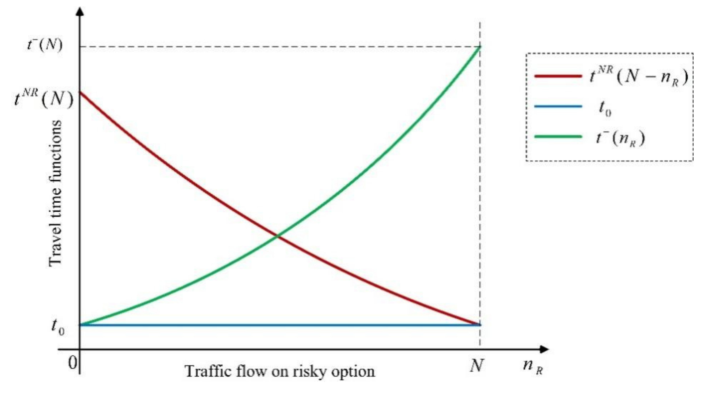
We assume N travelers go from the common origin, e.g., the suburb area, to the common destination, e.g., the core area, and study their bi-attribute (travel time and travel cost) risky mode choice behavior with one risky option, i.e., the highway, denoted by $R$, and one non-risky option, i.e., the transit, denoted by $NR$. Furthermore, we investigate its long-run effect and assume there is no other mode options, e.g., staying at home. As aforementioned, travelers mainly focus on these two travel modes in practice. There are two states of the world, say good state and bad state, and the set of states is denoted by $S$. We use $p\left(p\in \left(0,1\right)\right)$ to denote the probability of bad state and then $1-p$ is the probability of good state. When $p=0$ or $p=1$, the risky option degenerates into a non-risky option, which will not be discussed furthermore. On the non-risky option $NR$, the travel utility functions are the same for both states, denoted by $u^{NR}$, while the travel utility function on the risky option depends on the state, denoted by $u^{+}$ in the good state, and $u^{-}$ in the bad state.

The nonlinear travel utility functions shown in Equation (1) are used in our study, which are in the form of the difference between the utility value (due to the arrival at the destination) $U$ and the generalized cost (weighted sum of travel time and travel cost) between the origin and the destination. Moreover, we assume that travelers could specify a suitable value $U$ to make the utility functions always positive as [28] and [40].

$$\begin{array}{l}{u}^{+}\left(n_R\right)=U-\left[t_0+\beta {\tau }_1\right],\\ u^{-}\left(n_R\right)=U-\left[t^{-}\left(n_R\right)+\beta {\tau }_1\right],\\ u^{NR}\left(N-n_R\right)=U-\left[t^{NR}\left(N-n_R\right)+\beta {\tau }_2\right],\end{array}$$

(1)

where $n_R$ denotes the traffic flows on the risky option, and then travel flows on the non-risky option is $N-n_R$. Travel costs on these two options, risky and non-risky option, are ${\tau }_1$ and ${\tau }_2$, respectively, and $\beta >0$ denotes value of travel cost, which converts the travel cost into travel time. At the same time, $t^{-}\left(n_R\right)$ and $t^{NR}\left(N-n_R\right)$ are defined as travel time functions on the risky option and the non-risky option, respectively. In this paper, the travel time functions $t^{-}\left(n_R\right)$ and $t^{NR}\left(N-n_R\right)$ are considered to be a continuous strictly increasing function of the traffic volume on the corresponding option, and then we have $\frac{d{t}^{-}\left(n_R\right)}{d{n}_R}>0$ and $\frac{d{t}^{NR}\left(N-n_R\right)}{d{n}_R}<0$. In addition, it is assumed that $t^{-}\left(N\right)>t^{NR}\left(N\right)$, i.e., travel time of the risky option in bad state is larger than that of the non-risky option when the flow is N, and the free flow travel times $t_0$ on these two options are identical. Therefore, the bad state is the most undesirable. Finally, the utility in the good state of the risky option is a constant, which is normalized as $U-\left(t_0+\beta {\tau }_1\right)$. Assumptions made here could simplify our discussions in this paper, but our method can be extended accordingly if some assumptions are relaxed, and nevertheless, the insights and implications obtained according to our results will not be changed. The relationship between these travel time functions is shown in Figure 1.

3. Bi-Attribute Salient Travel Utility Model Based on Flow-Dependent Salience Theory

In this section, we introduce the flow-dependent salience theory first, and then propose the bi-attribute salient route utility model based on this theory.

3.1. Flow-Dependent Salience Theory

Following the principle of expected utility theory, the bi-attribute expected travel utility on the risky option is $\left(1-p\right)u^{+}\left(n_R\right)+p{u}^{-}\left(n_R\right)$, while the bi-attribute travel utility on the non-risky option is $u^{NR}\left(N-n_R\right)$. However, decision makers’ mind might focus on whatever is odd, unusual or different, which is the essential meaning of salience ([41]). Therefore, travelers could over-weight the route’s most salient states in $S$, and assign a subjective probability to each state s (good or bad state), which depends on the objective probability of the state s and its salience. To formally define the flow-dependent salience theory, let $u_s^{\max }$ and $u_s^{\min }$ denote the largest and smallest utilities for each state s, respectively, and $u_s^{-i}$ denote the utility of route $j,j\ne s$

Definition 1.

The salience of state$s$for option$i,i=R,NR$, is a continuous and bounded function$\sigma \left(u_s^i\left(n_R\right),u_s^{-i}\left(n_R\right)\right)$for a given flow$n_R$that satisfies the following two conditions:

1. 

Ordering. If for state$s,\tilde{s}\in S$we have that$\left[u_s^{\min }\left(n_R\right),u_s^{\max }\left(n_R\right)\right]$is a subset of$\left[u_{\tilde{s}}^{\min }\left(n_R\right),u_{\tilde{s}}^{\max }\left(n_R\right)\right]$, then

$$\sigma \left(u_s^i\left(n_R\right),u_s^{-i}\left(n_R\right)\right)<\sigma \left(u_{\tilde{s}}^i\left(n_R\right),u_{\tilde{s}}^{-i}\left(n_R\right)\right)$$

(2)

2. 

Diminishing sensitivity. If$u_s^i\left(n_R\right)>0fori=R,NR$, then for any$\epsilon >0$,

$$\sigma \left(u_s^i\left(n_R\right)+\epsilon ,u_s^{-i}\left(n_R\right)+\epsilon \right)<\sigma \left(u_s^i\left(n_R\right),u_s^{-i}\left(n_R\right)\right)$$

(3)

In the original salience theory ([18]), there is another property for the salience function, called reflection, which can handle negative utility. However, this property is not needed in our study, because all the values of utility functions are positive. To illustrate Definition (1), we use salience function

$$\sigma \left(u_s^i\left(n_R\right),u_s^{-i}\left(n_R\right)\right)=\frac{\left|u_s^i\left(n_R\right)-u_s^{-i}\left(n_R\right)\right|}{u_s^i\left(n_R\right)+u_s^{-i}\left(n_R\right)}$$

(4)

It can be verified that this salience function satisfies both properties used in Definition (1). For a given value of $n_R$, the ordering property shows that the difference between the utility $u_s^i\left(n_R\right)$ of option $u_s^{-i}\left(n_R\right)$ of other option increases, and thus the salience of the state s will increase, which is captured by $\left|u_s^i\left(n_R\right)-u_s^{-i}\left(n_R\right)\right|$. For a given value of $n_R$, the diminishing sensitivity property shows that if a state’s utility becomes larger, and thus the salience will decrease, which is captured by $u_s^i\left(n_R\right)-u_s^{-i}\left(n_R\right)$. Moreover, we see that the salience function (4) also satisfies the symmetry property, because we discuss the mode choice between two options. Particularly, given states $s,\tilde{s}\in S$, state $s$ is said to be more salient than $\tilde{s}$ for option $i\left(i=R,NR\right)$, if $\sigma \left(u_s^i\left(n_R\right),u_s^{-i}\left(n_R\right)\right)>\sigma \left(u_{\tilde{s}}^i\left(n_R\right),u_{\tilde{s}}^{-i}\left(n_R\right)\right)$.

We see that the travel utilities and the salience function are both flow-dependent, where the flow denotes the traffic flow on the risky option, and thus, we call it flow-dependent salience theory.

3.2. Bi-Attribute Salient Travel Utility Model

Based on the flow-dependent salience theory, we propose the bi-attribute salient travel utility model as follows.

Definition 2.

According to the flow-dependent salience theory, travelers evaluate the bi-attribute salient travel utility on the risky option according to the formulation

$$U^R\left(n_R\right)=\frac{{\delta }_1\left(1-p\right)u^{+}\left(n_R\right)+{\delta }_{2}p{u}^{-}\left(n_R\right)}{{\delta }_1\left(1-p\right)+{\delta }_{2}p}$$

(5)

while travelers evaluate the bi-attribute salient travel utility on the non-risky option according to the formulation

$$U^{NR}\left(n_R\right)=\frac{{\delta }_1\left(1-p\right)u^{NR}\left(N-n_R\right)+{\delta }_{2}p{u}^{NR}\left(N-n_R\right)}{{\delta }_1\left(1-p\right)+{\delta }_{2}p}=u^{NR}\left(N-n_R\right)$$

(6)

where${\delta }_1={\delta }^{-{\sigma }_1\left(u^{+}\left(n_R\right),u^{NR}\left(N-n_R\right)\right)}$, and${\delta }_2={\delta }^{-{\sigma }_2\left(u^{-}\left(n_R\right),u^{NR}\left(N-n_R\right)\right)}$.

According to Equation (4), we have

$$\begin{array}{ll}{\sigma }_1& =\frac{\left|u^{+}\left(n_R\right)-u^{NR}\left(N-n_R\right)\right|}{u^{+}\left(n_R\right)+u^{NR}\left(N-n_R\right)}\\ & =\frac{\left|t^{NR}\left(N-n_R\right)-t_0+\beta \left({\tau }_2-{\tau }_1\right)\right|}{2U-t^{NR}\left(N-n_R\right)-t_0-\beta \left({\tau }_2+{\tau }_1\right)}\end{array}$$

(7)

$$\begin{array}{ll}{\sigma }_2& =\frac{\left|u^{-}\left(n_R\right)-u^{NR}\left(N-n_R\right)\right|}{u^{-}\left(n_R\right)+u^{NR}\left(N-n_R\right)}\\ & =\frac{\left|t^{NR}\left(N-n_R\right)-t^{-}\left(n_R\right)+\beta \left({\tau }_2-{\tau }_1\right)\right|}{2U-t^{NR}\left(N-n_R\right)-t^{-}\left(n_R\right)-\beta \left({\tau }_2+{\tau }_1\right)}\end{array}$$

(8)

From Definition (2), we see that the bi-attribute salient travel utility on the risky option can be written as $\left(1-p^{\prime }\right)u^{+}\left(n_R\right)+p^{\prime }{u}^{-}\left(n_R\right)$, where $p^{\prime }=\frac{{\delta }_{2}p}{{\delta }_1\left(1-p\right)+{\delta }_{2}p}$, and the bi-attribute salient travel utility on the non-risky option remains the same, regardless of the composition of the choice set. Compared to the formulation for the bi-attribute expected utility theory, i.e., $\left(1-p\right)u^{+}\left(n_R\right)+p{u}^{-}\left(n_R\right)$, we see that the only difference is the change of the objective probability, which is called distorted probability for bad state and good state based on flow-dependent salience theory.

Parameter $\delta \left(\delta \in \left(0,1\right]\right)$ indicates travelers’ susceptibility to the salience, called salience bias. $\delta =1$ means rational travelers, and thus there is no distortion on the objective probabilities of the states. In the following study, when $\delta <1$, the travelers are called salient travelers. Smaller value of $\delta$ means stronger salience bias, and vice versa. In the special situation where $\delta \to 0$, the salient travelers will only pay their attention on the most bi-attribute salient travel utility.

Based on the bi-attribute salient route utility presented in Definition (2), we obtain the following proposition about the mode preference, which is basis of our equilibrium analysis.

Proposition 1.

For a given flow$n_R$, a salient traveler will choose the risky option if and only if the following inequality satisfied.

$${\delta }_1\left(1-p\right)\left[u^{+}\left(n_R\right)-u^{NR}\left(N-n_R\right)\right]+{\delta }_{2}p\left[u^{-}\left(n_R\right)-u^{NR}\left(N-n_R\right)\right]>0$$

(9)

Proof. 

For a given flow variable $n_R$, based on the bi-attribute salient travel utility, a salient traveler prefers the risky option to the non-risky option if and only if $U^R\left(n_R\right)>U^{NR}\left(n_R\right)$ i.e.,

$$\frac{{\delta }_1\left(1-p\right)\left[u^{+}\left(n_R\right)+{\delta }_{2}p{u}^{-}\left(n_R\right)\right]}{{\delta }_1\left(1-p\right)+{\delta }_{2}p}>u^{NR}\left(N-n_R\right)$$

(10)

Equation (9) can be obtained by Equation (10) after some rearrangement, which completes the proof. □

4. Bi-Attribute Salient User Equilibrium Analysis

In this section, we study the long-run effect of bi-attribute salient travel utility, and propose the bi-attribute salient user equilibrium (BaSUE), which can be stated as: No traveler can improve their bi-attribute salient travel utility by unilaterally changing their options. Furthermore, we compare the results of the BaSUE with those of bi-attribute expected user equilibrium (BaEUE), which can be stated as: No traveler can improve their bi-attribute expected travel utility by unilaterally changing their options.

Based on Proposition (1), we see that at the BaSUE, the following equation is satisfied.

$${\delta }_1\left(1-p\right)\left[u^{+}\left(n_R\right)-u^{NR}\left(N-n_R\right)\right]+{\delta }_{2}p\left[u^{-}\left(n_R\right)-u^{NR}\left(N-n_R\right)\right]=0$$

(11)

Furthermore, we define the following flow-dependent mode preference function based on Equation (11), which is the foundation of our equilibrium analysis.

Definition 3.

The flow-dependent mode preference function, denoted by$V_{R\to NR}\left(n_R\right)$is defined as

$$V_{R\to NR}\left(n_R\right)={\delta }_1\left(1-p\right)\left[u^{+}\left(n_R\right)-u^{NR}\left(N-n_R\right)\right]+{\delta }_{2}p\left[u^{-}\left(n_R\right)-u^{NR}\left(N-n_R\right)\right]$$

(12)

From Definition (3), we see that when $V_{R\to NR}\left(n_R\right)>0$, the salient travelers prefer the risky option to the non-risky option, when $V_{R\to NR}\left(n_R\right)<0$, the salient travelers prefer the non-risky option to the risky option, and when $V_{R\to NR}\left(n_R\right)=0$, the BaSUE is reached.

4.1. Formal Results on the BaSUE

Next, we present the formal analysis on the BaSUE, and before that, following the principle of expected utility theory, we present the analysis on the BaEUE as a benchmark case for comparison. We always use $n_{\mathrm{Re}}$ to denote the equilibrium flow on the risky option.

Proposition 2.

When$-\left[t^{NR}\left(N\right)-t_0\right]\ge \beta \left({\tau }_2-{\tau }_1\right)$, there exists a corner BaEUE, where$n_{\mathrm{Re}}=0$, and when$\beta \left({\tau }_2-{\tau }_1\right)\ge p\left[t^{-}\left(N\right)-t_0\right]$, there exists a corner BaEUE, where$n_{\mathrm{Re}}=N$.

Proof. 

The proof can be completed based on the following logic. A corner BaEUE is obtained when either of the following two conditions is satisfied.

1.

When $n_{\mathrm{R}}=0$, the bi-attribute expected travel utility of the risky option is still not greater than the travel utility of the non-risky option, i.e., $\left(1-p\right)u^{+}\left(0\right)+p{u}^{-}\left(0\right)\le u^{NR}\left(N\right)$. In this situation, we obtain that $n_{\mathrm{Re}}=0$ is a corner BaEUE. Substituting the travel utility functions into this inequality and rearranging it, we obtain $-\left[t^{NR}\left(N\right)-t_0\right]\ge \beta \left({\tau }_2-{\tau }_1\right)$.

2.

When $n_{\mathrm{R}}=N$, the bi-attribute expected travel utility of the risky option is still not less than the travel utility of the non-risky option, i.e., $\left(1-p\right)u^{+}\left(N\right)+p{u}^{-}\left(N\right)\le u^{NR}\left(0\right)$. In this situation, we obtain that $n_{\mathrm{Re}}=N$ is a corner BaEUE. Substituting the travel utility functions into this inequality and rearranging it, we obtain $p\left[t^{-}\left(N\right)-t_0\right]\le \beta \left({\tau }_2-{\tau }_1\right)$. □

The intuitive interpretation on Proposition (2) is that when the travel cost of one option is too large (or too small) compared to that of the other option, travelers’ mode choice decisions cannot be changed, even though increase in traffic flow causes the increase in travel time. That is, when the travel cost of a certain option is too large, no matter how the traffic flow is distributed, travelers will choose the option with a small travel cost, and vice versa. According to this proposition, we only discuss the situations where $-\left[t^{NR}\left(N\right)-t_0\right]<\beta \left({\tau }_2-{\tau }_1\right)<p\left[t^{-}\left(N\right)-t_0\right]$ is satisfied.

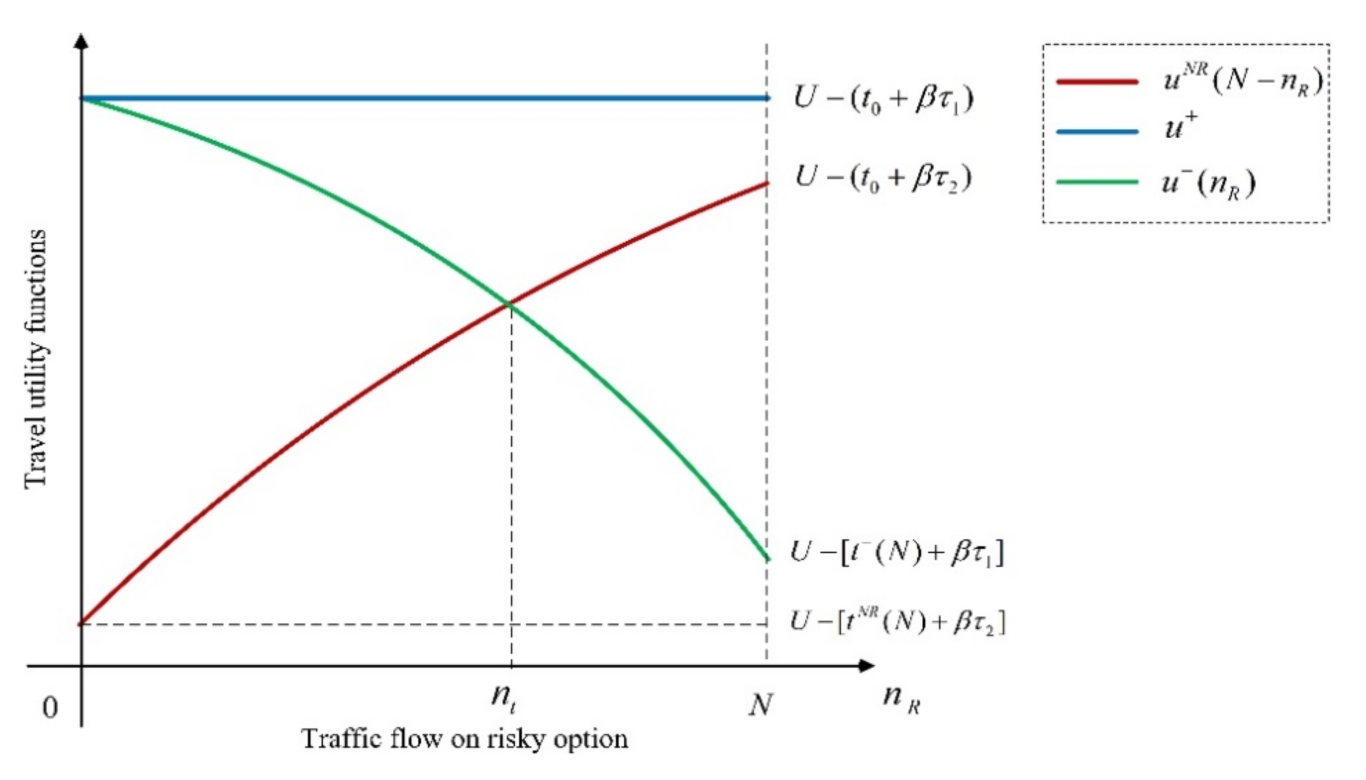
Surprisingly, result in Proposition (2) is also a sound prerequisite for the analysis on BaSUE due to the inherent relationship between the expected utility theory and salience theory as discussed in the part of flow-dependent salience theory, which will be elaborated in the following discussions. We divide the condition $-\left[t^{NR}\left(N\right)-t_0\right]<\beta \left({\tau }_2-{\tau }_1\right)<p\left[t^{-}\left(N\right)-t_0\right]$ into two cases, and the motivation for this division is the utility value when the flow on each option is N.

1.

Case 1: $0<\beta \left({\tau }_2-{\tau }_1\right)<p\left[t^{-}\left(N\right)-t_0\right]$. In this case, the corresponding relationship between different travel utility functions is shown in Figure 2 schematically. We see that when the flow on each option is N, $u^{+}\left(N\right)\ge u^{NR}\left(N\right)>u^{-}\left(N\right)$ is satisfied. The relationship $u^{+}\left(N\right)=u^{NR}\left(N\right)$ when ${\tau }_1={\tau }_2$ is not shown explicitly, and one can modify Figure 2 for this straightforwardly. Moreover, relationship $u^{+}\left(N\right)=u^{NR}\left(N\right)$ can also be incorporated into Case 2 without loss of generality.

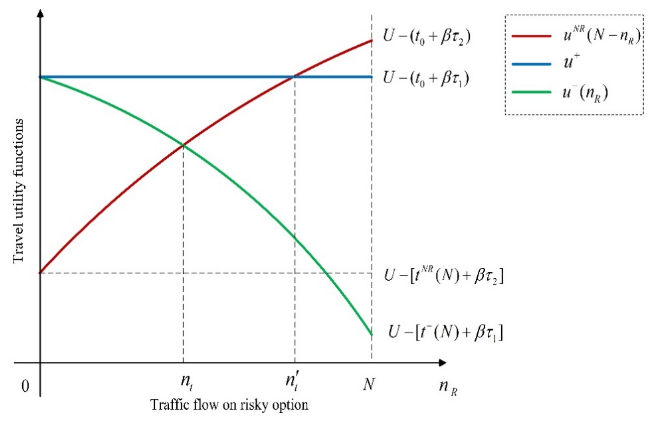
2.

Case 2: $-\left[t^{NR}\left(N\right)-t_0\right]<\beta \left({\tau }_2-{\tau }_1\right)<0$. In this case, the corresponding relationship between different travel utility functions is shown in Figure 3 schematically. We see that when the flow on each option is N, $u^{NR}\left(N\right)>u^{+}\left(N\right)>u^{-}\left(N\right)$ is satisfied.

From Figure 2 and Figure 3, we see that when $n_{\mathrm{R}}\in \left[0,n_t\right]$ (here, $n_t$ denotes the temporary value of $n_R$, and is obtained by solving the equation $u^{-}\left(n_R\right)-u^{NR}\left(N-n_R\right)=0$), $u^{+}\left(n_R\right)-u^{NR}\left(N-n_R\right)>0$ and $u^{-}\left(n_R\right)-u^{NR}\left(N-n_R\right)\ge 0$). Substituting these two inequalities into the flow-dependent mode preference function and with ${\delta }_1$ and ${\delta }_2$ being positive, we have

$$V_{R\to NR\left(n_R\right)}={\delta }_1\left(1-p\right)\left[u^{+}\left(n_R\right)-u^{NR}\left(N-n_R\right)\right]+{\delta }_{2}p\left[u^{-}\left(n_R\right)-u^{NR}\left(N-n_R\right)\right]>0$$

(13)

i.e., the salient travelers always prefer the risky option to the non-risky option. Therefore, we obtain that when $n_R\in \left[0,n_t\right]$, there is no BaSUE. The aforementioned discussions are true for both cases, while for Case 2, we can obtain more results.

When $n_R\in \left[{n^{\prime }}_t,N\right]$, N] (here, ${n^{\prime }}_t$ also denotes the temporary value of $n_R$, and is obtained by solving the equation $u^{+}\left(n_R\right)-u^{NR}\left(N-n_R\right)=0$), we have $u^{+}\left(n_R\right)-u^{NR}\left(N-n_R\right)\le 0$ and $u^{-}\left(n_R\right)-u^{NR}\left(N-n_R\right)<0$. Substituting these two inequalities into the flow-dependent mode preference function and with ${\delta }_1$ and ${\delta }_2$ being positive, we have

$$V_{R\to NR\left(n_R\right)}={\delta }_1\left(1-p\right)\left[u^{+}\left(n_R\right)-u^{NR}\left(N-n_R\right)\right]+{\delta }_{2}p\left[u^{-}\left(n_R\right)-u^{NR}\left(N-n_R\right)\right]<0$$

(14)

i.e., the salient travelers always prefer the non-risky option to the risky option. Therefore, we obtain that when $n_R\in \left[{n^{\prime }}_t,N\right]$, there is no BaSUE. Therefore, in the following discussions, we only consider interval $\left(n_t,N\right]$ for Case 1, and interval $\left(n_t,{n^{\prime }}_t\right)$ for Case 2.

Next we discuss the BaSUE in these two cases separately based on the following technical lemma.

Lemma 1.

The flow-dependent mode preference function$V_{R\to NR\left(n_R\right)}$is a strictly decreasing function of the flow$n_R$in the considered interval$\left(n_t,N\right]$or$\left(n_t,{n^{\prime }}_t\right)$.

Proof. 

We prove this lemma is true for interval $\left(n_t,{n^{\prime }}_t\right)$, and the proof for interval $\left(n_t,N\right]$ can be completed similarly, which is omitted for brevity. □

It is obvious that in the interval $\left(n_t,{n^{\prime }}_t\right)$, $V_{R\to NR\left(n_R\right)}$ is continuous. The derivative of $V_{R\to NR\left(n_R\right)}$ is

$$\begin{array}{l}\frac{d{V}_{R\to NR\left(n_R\right)}}{d{n}_R}=\left(1-p\right){\delta }_1\left[-\ln \delta \frac{d{\sigma }_1}{d{n}_R}\left(t^{NR}\left(N-n_R\right)-t_0+\beta \left({\tau }_2-{\tau }_1\right)\right)+\frac{d{t}^{NR}\left(N-n_R\right)}{d{n}_R}\right]+\\ p{\delta }_2\left[-\ln \delta \frac{d{\sigma }_2}{d{n}_R}\left(t^{NR}\left(N-n_R\right)-t^{-}\left(n_R\right)+\beta \left({\tau }_2-{\tau }_1\right)\right)+\left(\frac{d{t}^{NR}\left(N-n_R\right)}{d{n}_R}-\frac{d{t}^{-}\left(n_R\right)}{d{n}_R}\right)\right]\end{array}$$

To prove the strict monotonicity of the flow-dependent mode preference function, the following steps are followed. When $n_R\left(n_t,{n^{\prime }}_t\right)$${\sigma }_1=\frac{t^{NR}\left(N-n_R\right)-t_0+\beta \left({\tau }_2-{\tau }_1\right)}{2U-t^{RN}\left(N-n_R\right)-t_0-\beta \left({\tau }_2+{\tau }_1\right)}$, and thus $\frac{d{\sigma }_1}{d{n}_R}=2\frac{\frac{d{t}^{NR}\left(N-n_R\right)}{d{n}_R}\left[U-\left(t_0+\beta {\tau }_1\right)\right]}{{\left[2U-t^{NR}\left(N-n_R\right)-t_0-\beta \left({\tau }_2+{\tau }_1\right)\right]}^2}$. Because $\frac{d{t}^{NR}\left(N-n_R\right)}{d{n}_R}<0$ and $\left[U-\left(t_0+\beta {\tau }_1\right)\right]>0$, we obtain $\frac{{d\sigma }_2}{d{n}_R}>0$.

When $n_R\left(n_t,{n^{\prime }}_t\right),{\sigma }_1=\frac{t^{-}\left(n_R\right)-t^{NR}\left(N-n_R\right)-\beta \left({\tau }_2-{\tau }_1\right)}{2U-t^{RN}\left(N-n_R\right)-t^{-}\left(n_R\right)-\beta \left({\tau }_2+{\tau }_1\right)}$, and thus

$\frac{d{\sigma }_2}{d{n}_R}=-2\frac{\frac{d{t}^{NR}\left(N-n_R\right)}{d{n}_R}\left[U-\left(t^{-}\left(n_R\right)+\beta {\tau }_1\right)\right]-\frac{d{t}^{-}\left(n_R\right)}{d{n}_R}\left[U-\left(t^{NR}\left(N-n_R\right)+\beta {\tau }_2\right)\right]}{{\left[2U-t^{NR}\left(N-n_R\right)-t^{-}\left(n_R\right)-\beta \left({\tau }_2+{\tau }_1\right)\right]}^2}$. Because $\frac{d{t}^{NR}\left(N-n_R\right)}{d{n}_R}<0$, $\frac{d{t}^{-}\left(n_R\right)}{d{n}_R}>0$, $U-\left(t^{-}\left(n_R\right)+\beta {\tau }_1\right)>0$, and $U-\left(t^{NR}\left(N-n_R\right)+\beta {\tau }_2\right)>0$, we obtain $\frac{d{\sigma }_2}{d{n}_R}>0$.

From Figure 3, we see that $u^{+}\left(n_R\right)-u^{NR}\left(N-n_R\right)>0$,$u^{-}\left(n_R\right)-u^{NR}\left(N-n_R\right)<0$ when $n_R\in \left(n_t,{n^{\prime }}_t\right)$, which can also be verified with the travel utility functions. Therefore $\frac{d{\sigma }_1}{d{n}_R}=t^{NR}\left(N-n_R\right)-t_0+\beta \left({\tau }_2-{\tau }_1\right)<0$ and $\frac{d{\sigma }_2}{d{n}_R}=t^{NR}\left(N-n_R\right)-t^{-}\left(n_R\right)+\beta \left({\tau }_2-{\tau }_1\right)<0$, $\delta \in \left(0,1\right)$ implies $\ln \delta <0$ and we have ${\delta }_1>0$ and ${\delta }_2>0$.

Combining all these results, we can show that $\frac{d{V}_{R\to NR\left(n_R\right)}}{d{n}_R}<0,\forall n_R\in \left(n_t,{n^{\prime }}_t\right)$.

4.1.1. Case 1

In this case, $0\le \beta \left({\tau }_2-{\tau }_1\right)<p\left[t^{-}\left(N\right)-t_0\right]$ is satisfied, which corresponds to Figure 2, and we present the formal results on the equilibrium in this section.

The right-hand side of this inequality is the value when $n_R=N$ with the objective probability, which motivates us to discuss the value when $n_R=N$ with the distorted probability.

When $n_R=N$, one of three possible situations can happen given the specific travel utility functions. If ${\sigma }_1\left(u^{+}\left(N\right),u^{NR}\left(0\right)\right)<{\sigma }_2\left(u^{-}\left(N\right),u^{NR}\left(0\right)\right)$, i.e., bad state is salient (Recall that $\delta \in \left(0,1\right),{\delta }_1>{\delta }_2$. Similarly, we obtain when ${\sigma }_1\left(u^{+}\left(N\right),u^{NR}\left(0\right)\right)>{\sigma }_2\left(u^{-}\left(N\right),u^{NR}\left(0\right)\right)$ i.e., good state is salient, ${\delta }_1<{\delta }_2$, and when ${\sigma }_1\left(u^{+}\left(N\right),u^{NR}\left(0\right)\right)={\sigma }_2\left(u^{-}\left(N\right),u^{NR}\left(0\right)\right)$, i.e., no state is salient, ${\delta }_1={\delta }_2$.

If $\delta \in \left(0,1\right),{\delta }_1>{\delta }_2$, we have $\frac{{\delta }_{2}p}{{\delta }_1\left(1-p\right)+{\delta }_{2}p}<\frac{{\delta }_{2}p}{{\delta }_2\left(1-p\right)+{\delta }_{2}p}=p$ i.e., the distorted probability is strictly less than the objective probability. Similarly, if ${\delta }_1={\delta }_2$, we have $\frac{{\delta }_{2}p}{{\delta }_1\left(1-p\right)+{\delta }_{2}p}=p$, and if ${\delta }_1<{\delta }_2$, we have $\frac{{\delta }_{2}p}{{\delta }_1\left(1-p\right)+{\delta }_{2}p}>p$.

Next, we discuss the three possible situations separately.

Proposition 3.

If${\delta }_1>{\delta }_2$when$n_R=N$, there is a unique BaSUE between$n_t$and$N$. In particular, the cost difference, which ensures that there is still no corner equilibrium, becomes smaller.

Proof. 

We complete the first part of the proof in two steps. When $\frac{{\delta }_{2}p}{{\delta }_1\left(1-p\right)+{\delta }_{2}p}\left[t^{-}\left(N\right)-t_0\right]<\beta \left({\tau }_2-{\tau }_1\right)$, we have

$$\begin{array}{cc}\hfill & V_{R\to NR}\left(N\right)=p{\delta }_2\left[t_0-t^{-}\left(N\right)+\beta \left({\tau }_2-{\tau }_1\right)\right]+\left(1-p\right){\delta }_1\left[\beta \left({\tau }_2-{\tau }_1\right)\right]\hfill \\ \hfill & >p{\delta }_2\left[t_0-t^{-}\left(N\right)+\frac{{\delta }_{2}p}{{\delta }_1\left(1-p\right)+{\delta }_{2}p}\left[t^{-}\left(N\right)-t_0\right]\right]+\left(1-p\right){\delta }_1\left[\frac{{\delta }_{2}p}{{\delta }_1\left(1-p\right)+{\delta }_{2}p}\left[t^{-}\left(N\right)-t_0\right]\right]\hfill \\ \hfill & =p{\delta }_2\frac{{\delta }_1\left(1-p\right)\left[t_0-t^{-}\left(N\right)\right]}{{\delta }_1\left(1-p\right)+{\delta }_{2}p}+\left(1-p\right){\delta }_1\left[\frac{{\delta }_{2}p}{{\delta }_1\left(1-p\right)+{\delta }_{2}p}\left[t^{-}\left(N\right)-t_0\right]\right]\hfill \\ \hfill & =0\hfill \end{array}$$

(15)

Therefore, the salient travelers always prefer the risky option. That is, there is no BaSUE when $\frac{{\delta }_{2}p}{{\delta }_1\left(1-p\right)+{\delta }_{2}p}\left[t^{-}\left(N\right)-t_0\right]<\beta \left({\tau }_2-{\tau }_1\right)<p\left(t^{-}\left(N\right)-t_0\right)$.

When $0\le \beta \left({\tau }_2-{\tau }_1\right)\le \frac{{\delta }_{2}p}{{\delta }_1\left(1-p\right)+{\delta }_{2}p}\left[t^{-}\left(N\right)-t_0\right]$, there is a unique BaSUE between $n_t$ and $N$. It can be verified that $\frac{{\delta }_{2}p}{{\delta }_1\left(1-p\right)+{\delta }_{2}p}\left[t^{-}\left(N\right)-t_0\right]=\beta \left({\tau }_2-{\tau }_1\right)$, i.e., $V_{R\to NR}\left(N\right)=0$. Following the similar steps used in the proof of Lemma (1), we obtain $\frac{d{V}_{R\to NR}\left(n_R\right)}{d{n}_R}<0,\forall n_R\in \left(n_t,N\right)$. Combining the results that $V_{R\to NR}\left(n_t\right)>0$ and $V_{R\to NR}\left(N\right)\le 0$, we can show that there is a unique value of $n_R\in \left(n_t,N\right]$ that satisfies $V_{R\to NR}\left(n_{\mathrm{Re}}\right)=0$, which completes the first part of the proof.□

Finally, $\frac{{\delta }_{2}p}{{\delta }_1\left(1-p\right)+{\delta }_{2}p}<p$ means that the cost difference, which ensures that there is still no corner equilibrium, becomes smaller.

Proposition 4.

If${\delta }_1={\delta }_2$when$n_R=N$, there is a unique BaSUE between$n_t$ and $N$. In particular, the cost difference, which ensures that there is still no corner equilibrium, remains the same.

Proof. 

If ${\delta }_1={\delta }_2$ when $n_R=N$, the BaSUE becomes the BaEUE. Follow the aforementioned discussions, we have $\frac{d{V}_{R\to NR}\left(n_R\right)}{d{n}_R}<0,\forall n_R\in \left(n_t,N\right)$. Combining the results that $V_{R\to NR}\left(n_t\right)>0$ and $V_{R\to NR}\left(N\right)\le 0$, we complete the first part of the proof. □

Finally, $\frac{{\delta }_{2}p}{{\delta }_1\left(1-p\right)+{\delta }_{2}p}=p$ means that the cost difference, which ensures that there is still no corner equilibrium, remains the same.

Proposition 5.

If${\delta }_1<{\delta }_2$when$n_R=N$, there is a unique BaSUE between$n_t$and$N$. In particular, we can increase the cost difference, and meanwhile, guarantee that there is still no corner equilibrium.

Proof. 

If ${\delta }_1<{\delta }_2$ when $n_R=N$, we have

$$\beta \left({\tau }_2-{\tau }_1\right)<p\left[t^{-}\left(N\right)-t_0\right]<\frac{{\delta }_{2}p}{{\delta }_1\left(1-p\right)+{\delta }_{2}p}\left[t^{-}\left(N\right)-t_0\right]$$

Follow the aforementioned discussions, we have $\frac{d{V}_{R\to NR}\left(n_R\right)}{d{n}_R}<0,\forall n_R\in \left(n_t,N\right)$. Combining the results that $V_{R\to NR}\left(n_t\right)>0$ and $V_{R\to NR}\left(N\right)\le 0$, we complete the first part of the proof. □

Finally, $\frac{{\delta }_{2}p}{{\delta }_1\left(1-p\right)+{\delta }_{2}p}>p$ means that we can increase the cost difference, and meanwhile, guarantee that there is still no corner equilibrium.

All the results in the above three propositions about the corner equilibrium can be verified with the logic discussed in Proposition (2), by replacing the objective probability $p$ with the distorted probability $p^{\prime }$.

4.1.2. Case 2

In this case, $-\left[t^{NR}\left(N\right)-t_0\right]<\beta \left({\tau }_2-{\tau }_1\right)<0$ is satisfied, which corresponds to Figure 3, and we present the formal results on the equilibrium in this section. In this case, there is no objective probability p on left-hand side of the inequality, which is different from that in Case 1.

Proposition 6.

There is a unique BaSUE$n_{\mathrm{Re}}$between$n_t$ and ${n^{\prime }}_t$.

Proof. 

$V_{R\to NR}\left(n_t\right)={\delta }_1\left(1-p\right)\left[u^{+}\left(n_t\right)-u^{NR}\left(N-n_t\right)\right]>0$,$V_{R\to NR}\left({n^{\prime }}_t\right)={\delta }_{2}p\left[u^{-}\left({n^{\prime }}_t\right)-u^{NR}\left(N-{n^{\prime }}_t\right)\right]<0$, combining these results in Lemma (1), we obtain that there is a unique value of $n_R\in \left(n_t,{n^{\prime }}_t\right)$ hat satisfies $V_{R\to NR}\left(n_{\mathrm{Re}}\right)=0$, which completes the proof. □

4.2. Travelers’ Risk Attitude on the Bi-Attribute Risky Mode Choice

In this section, we present the results on travelers’ attitude based on the BaSUE.

Theorem 1.

At the equilibrium, if no state is salient, i.e.,${\delta }_1={\delta }_2$, travelers are risk-neutral; if good state is salient, i.e.,${\delta }_1<{\delta }_2$, travelers are risk-seeking; if bad state is salient, i.e.,${\delta }_1>{\delta }_2$, travelers are risk-averse.

Proof. 

At the BaSUE, if no state is salient, we have ${\delta }_1={\delta }_2$, and thus Equation (13) becomes $p{\delta }_1\left(1-p\right)\left[u^{-}\left(n_R\right)-u^{NR}\left(n_R\right)\right]+\left(1-p\right){\delta }_1\left[u^{+}\left(n_R\right)-u^{NR}\left(n_R\right)\right]=0$. Then we have $p\left[u^{-}\left(n_R\right)-u^{NR}\left(n_R\right)\right]+\left(1-p\right)\left[u^{+}\left(n_R\right)-u^{NR}\left(n_R\right)\right]=0$, i.e.,

$$p{u}^{-}\left(n_R\right)+\left(1-p\right)u^{+}\left(n_R\right)=0$$

(16)

Therefore, we obtain the BaEUE. The distorted probability of good state will become larger if it is salient, which will increase the left-hand-side value of Equation (16). Therefore, more travelers will choose the risky option, i.e., they are risk-seeking. Similarly, the distorted probability of the bad state will become larger if it is salient, which will decrease the left-hand-side value of Equation (16). Therefore, more travelers will choose the non-risky option, i.e., they are risk-averse. □

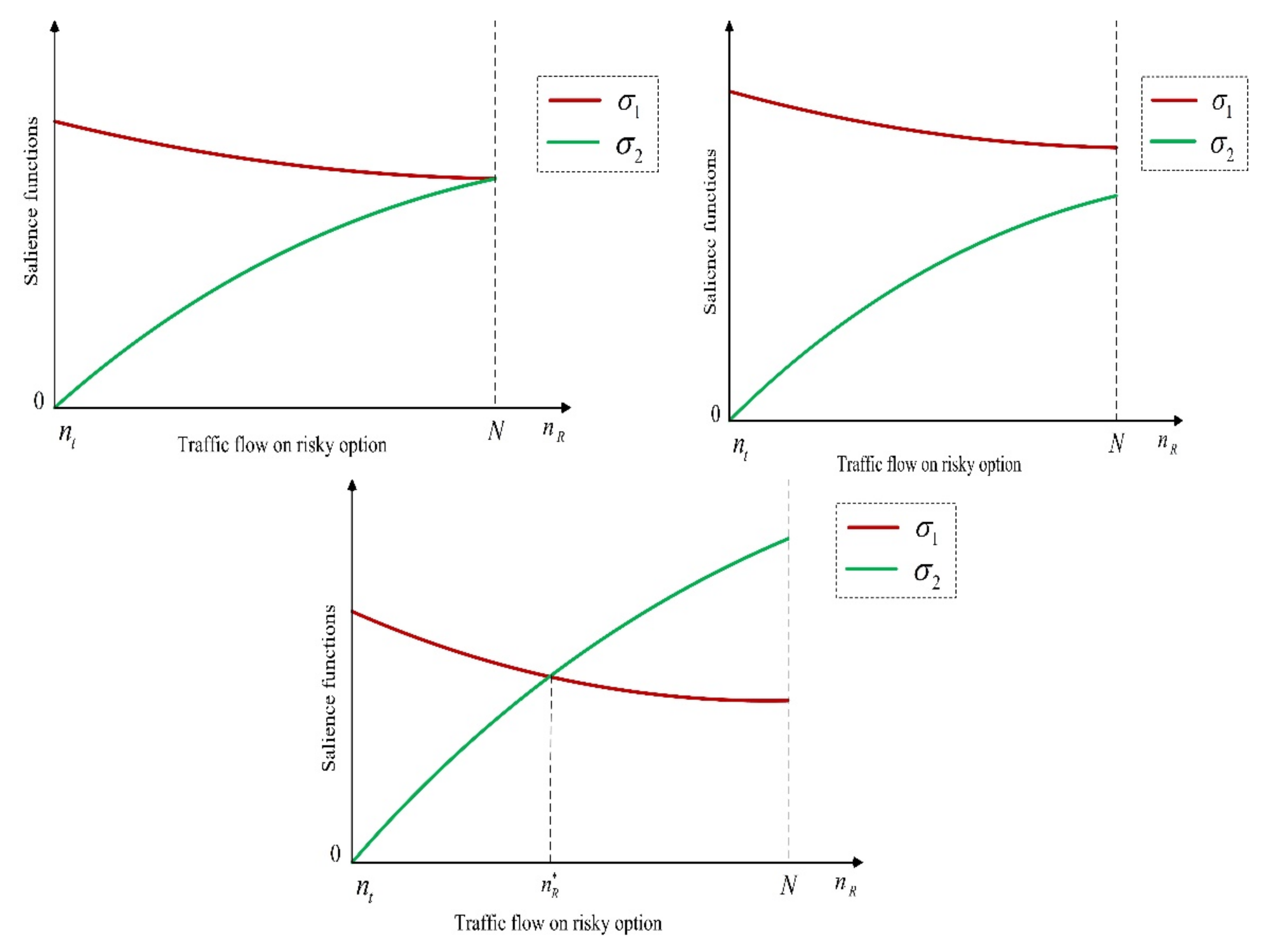
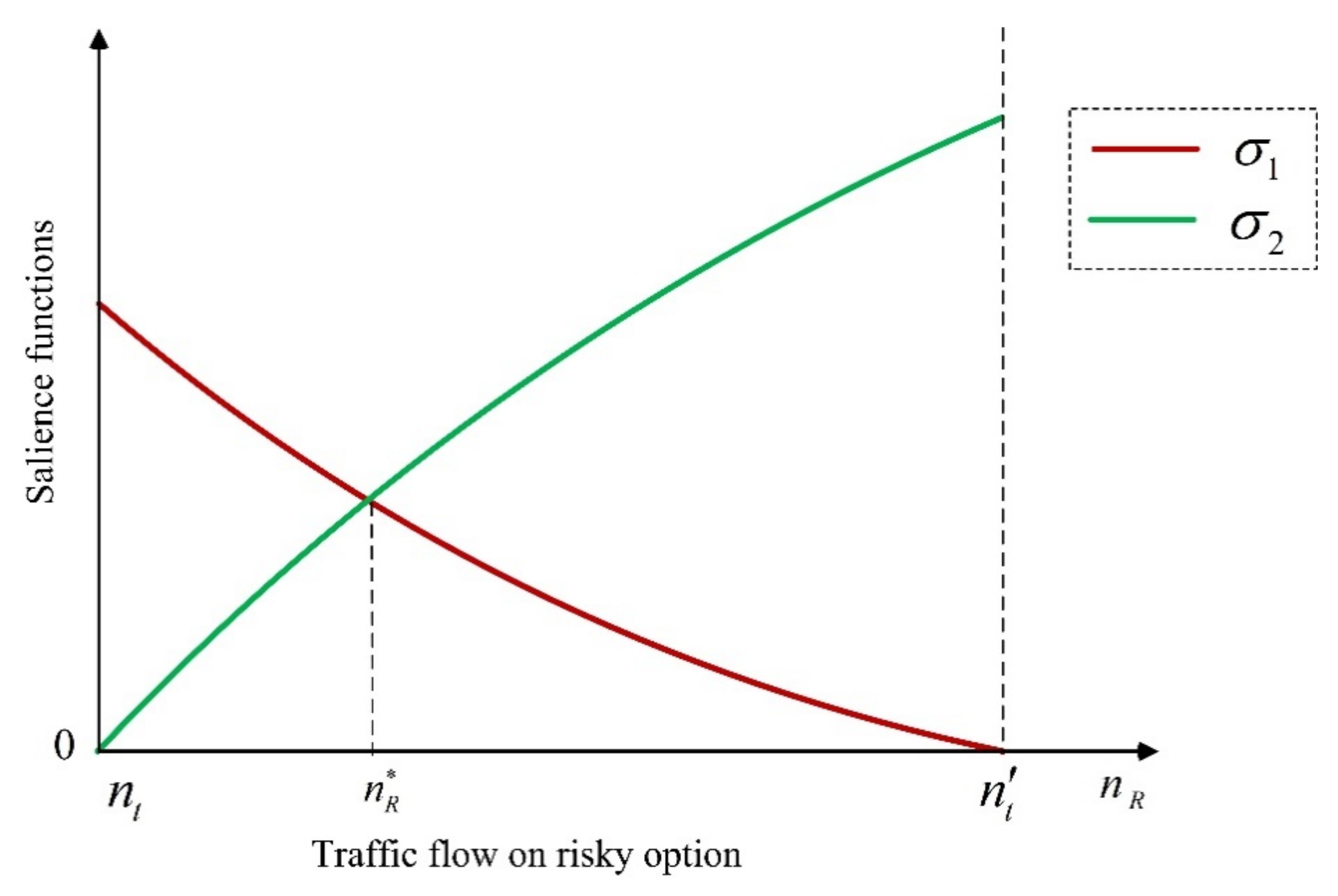
In practice, maybe only one state is salient for a specific situation, as shown in the following Figure 4. Next, we propose the flow-dependent salience ranking analysis to present more detailed results based on Theorem (1), and obtain the following two propositions. Result in Proposition (7) is motivated by the discussion on the BaSUE in Case 1, where the relationship between ${\delta }_1$ and ${\delta }_2$ is a key prerequisite when $n_R=N$. Here, we discuss the conditions for this relationship.

When $n_R=N$, we have ${\sigma }_1=\frac{\beta \left({\tau }_2-{\tau }_1\right)}{2U-2t_0-\beta \left({\tau }_2+{\tau }_1\right)}$ and ${\sigma }_2=\frac{t^{-}\left(N\right)-t_0-\beta \left({\tau }_2-{\tau }_1\right)}{2U-t_0-t^{-}\left(N\right)-\beta \left({\tau }_2+{\tau }_1\right)}$. If ${\sigma }_1<(=,>){\sigma }_2$ (see Figure 4), we obtain

$$\frac{\beta \left({\tau }_2-{\tau }_1\right)}{2U-2t_0-\beta \left({\tau }_2+{\tau }_1\right)}<\left(=,>\right)\frac{t^{-}\left(N\right)-t_0-\beta \left({\tau }_2-{\tau }_1\right)}{2U-t_0-t^{-}\left(N\right)-\beta \left({\tau }_2+{\tau }_1\right)}$$

(17)

Equation (17) can be seen as the sufficient conditions to figure out the salient state when $n_R=N$.

With the sufficient conditions, we obtain the following proposition.

Proposition 7.

In the case that$0\le \beta \left({\tau }_2-{\tau }_1\right)<p\left(t^{-}\left(N\right)-t_0\right)$, one of the following three situations can happen given the travel utility functions.

1. 

${\sigma }_1\left(N\right)<{\sigma }_2\left(N\right)$is satisfied, and then we can find an$n_R^{*}\in \left(n_t,N\right)$. When$n_R\in \left(n_t,n_R^{*}\right)$,${\sigma }_1>{\sigma }_2$, i.e., good state is salient and travelers are risk-seeking; when$n_R\in \left(n_R^{*},N\right)$,${\sigma }_2>{\sigma }_1$, i.e., bad state is salient and travelers are risk-averse; when$n_R=n_R^{*},{\sigma }_1={\sigma }_2$, i.e., no state is salient and travelers are risk-neutral.

2. 

${\sigma }_1\left(N\right)={\sigma }_2\left(N\right)$is satisfied, and then when$n_R^{}\in \left(n_t,N\right),{\sigma }_1>{\sigma }_2$, i.e., good state is salient and travelers are risk-seeking, and when$n_R=N,{\sigma }_1={\sigma }_2$, i.e., no state is salient and travelers are risk-neutral.

3. 

${\sigma }_1\left(N\right)>{\sigma }_2\left(N\right)$is satisfied, and then when$n_R\in \left(n_t,N\right],{\sigma }_1>{\sigma }_2$, i.e., good state is salient and travelers are risk-seeking.

Proof. 

According to the aforementioned discussions in Lemma (1), ${\sigma }_1\left(n_R\right)$ and ${\sigma }_2\left(n_R\right)$ are both continuous functions of $n_R$. $\frac{d{\sigma }_1}{d{n}_R}<0,\forall n_R\in \left(n_t,N\right]$, i.e., ${\sigma }_1$ is a strictly decreasing function of $n_R$ when $n_R\in \left(n_t,N\right]$, and $\frac{d{\sigma }_2}{d{n}_R}>0,\forall n_R\in \left(n_t,N\right]$, i.e.,${\sigma }_2$ is a strictly increasing function of $n_R$ when $n_R\in \left(n_t,N\right]$ We have discussed the relationship between ${\sigma }_1$ and ${\sigma }_2$ when $n_R=N$. With the strict monotonicity properties, we need to figure out the relationship between ${\sigma }_1$ and ${\sigma }_2$ when $n_R=n_t$. Recalling that $n_t$ is obtained by solving the equation $u^{-}\left(n_R\right)-u^{NR}\left(N-n_R\right)=0$, we have ${\sigma }_2\left(n_t\right)=0$ and ${\sigma }_1\left(n_t\right)>0$ by Equations (7) and (8). Therefore, combining all the results, we obtain the following three possible situations.

(a)

${\sigma }_1\left(N\right)<{\sigma }_2\left(N\right)$ as schematically shown in the upper-left figure of Figure 4. Then there exists $n_R^{*}\in \left(n_t,N\right)$. When $n_R^{}\in \left(n_t,n_R^{*}\right),{\sigma }_1>{\sigma }_2$, when $n_R^{}\in \left(n_R^{*},N\right),{\sigma }_2>{\sigma }_1$, when $n_R^{}=n_R^{*},{\sigma }_2={\sigma }_1$.

(b)

${\sigma }_1\left(N\right)={\sigma }_2\left(N\right)$ as schematically shown in the upper-right figure of Figure 4. When $n_R^{}\in \left(n_t,N\right)$${\sigma }_1>{\sigma }_2$ and when $n_R^{}=N,{\sigma }_1={\sigma }_2$.

(c)

${\sigma }_1\left(N\right)>{\sigma }_2\left(N\right)$ as schematically shown in the bottom figure of Figure 4. When $n_R^{}\in \left(n_t,N\right],{\sigma }_1>{\sigma }_2$. Combining with the results in Theorem (1), we complete the proof. □

Next, we talk about another case, i.e., Case 2.

Proposition 8.

In the case that$-\left[t^{NR}\left(N\right)-t_0\right]<\beta \left({\tau }_2-{\tau }_1\right)<0$, we can find an$n_R^{*}\in \left(n_t,{n^{\prime }}_t\right)$. When$n_R^{}\in \left(n_t,n_R^{*}\right),{\sigma }_1>{\sigma }_2$, i.e., good state is salient and travelers are risk-seeking; when$n_R^{}\in \left(n_R^{*},n^{\prime }\right),{\sigma }_2>{\sigma }_1$, i.e., bad state is salient and travelers are risk-averse; when$n_R^{}=n_R^{*},{\sigma }_1={\sigma }_2$, i.e., no state is salient and travelers are risk-neutral.

Proof. 

It is obvious that in the interval $\left(n_t,{n^{\prime }}_t\right)$, ${\sigma }_1\left(n_R\right)$ and ${\sigma }_2\left(n_R\right)$ are both continuous functions of $n_R$. We have ${\sigma }_1=\frac{t^{NR}\left(N-n_R\right)-t_0+\beta \left({\tau }_2-{\tau }_1\right)}{2U-t^{NR}\left(N-n_R\right)-t_0-\beta \left({\tau }_2+{\tau }_1\right)}$,${\sigma }_2=\frac{t^{-}\left(n_R\right)-t^{NR}\left(N-n_R\right)-\beta \left({\tau }_2-{\tau }_1\right)}{2U-t^{NR}\left(N-n_R\right)-t^{-}\left(n_R\right)-\beta \left({\tau }_2+{\tau }_1\right)}$, when $n_R\in \left(n_t,{n^{\prime }}_t\right)$. According to Lemma (1),$\frac{d{\sigma }_1}{d{n}_R}<0,\forall n_R\in \left(n_t,{n^{\prime }}_t\right)$,i.e.,${\sigma }_1$ is a strictly decreasing function of $n_R$ when $n_R\in \left(n_t,{n^{\prime }}_t\right)$, and $\frac{d{\sigma }_2}{d{n}_R}>0,\forall n_R\in \left(n_t,{n^{\prime }}_t\right)$, i.e., ${\sigma }_2$ is a strictly increasing function of $n_R$ when $n_R\in \left(n_t,{n^{\prime }}_t\right)$. Moreover, when $n_R=n_t$, we have ${\sigma }_2\left(n_t\right)=0$ and ${\sigma }_1\left(n_t\right)>0$; when $n_R={n^{\prime }}_t$, ${\sigma }_2\left({n^{\prime }}_t\right)=0$ and ${\sigma }_1\left({n^{\prime }}_t\right)=0$, recalling the calculation of ${n^{\prime }}_t$. Therefore, there is a value between $n_t$ and ${n^{\prime }}_t$, defined as $n_R^{*}$, that ${\sigma }_1={\sigma }_2$, as schematically shown in Figure 5. Furthermore, when $n_R\in \left(n_t,n_R^{*}\right)$, ${\sigma }_1>{\sigma }_2$; when $n_R\in \left(n_R^{*},{n^{\prime }}_t\right)$, ${\sigma }_2>{\sigma }_1$. Combining with the results in Theorem (1), we complete the proof. □

5. Numerical Examples

In this section, we conduct the numerical examples to show the performance of the proposed method, focusing on the sensitivity of equilibrium solution to the input parameters, the cost difference and the salience bias. We assume that there are $N=3000$ travelers in the system, and use the following quadratic travel utility functions.

$$u=U-\left(t_0+a{t}_0{\left(\frac{f}{Q}\right)}^2+\beta \tau \right)$$

(18)

where f denotes the traffic flow, $Q$ denotes the capacity, $t_0$ denotes the free-flow travel time, and parameters $a=0.15$. The free-flow travel times on both options are 80, and the capacity of risky option and non-risky option are 1000 and 1200, respectively. The intrinsic value $U$ is 205, and the value of travel cost $\beta$ is 0.5. We change the value of $p$ from 0 to 1, and use the linspace function in Matlab to generate 51 representative values. All the flow-dependent mode choice functions are solved with solve function in Matlab 2014a. We run the numerical examples for each case.

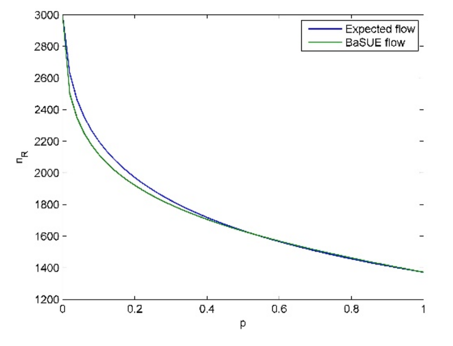
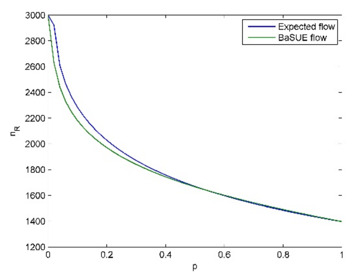
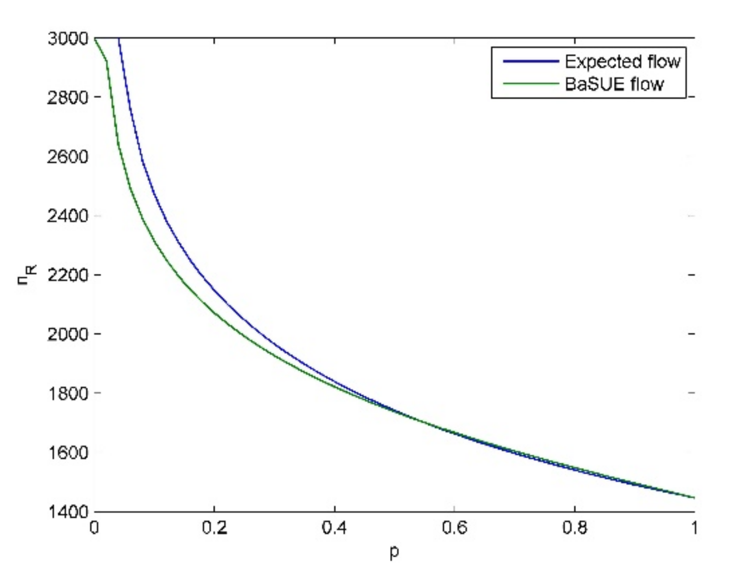
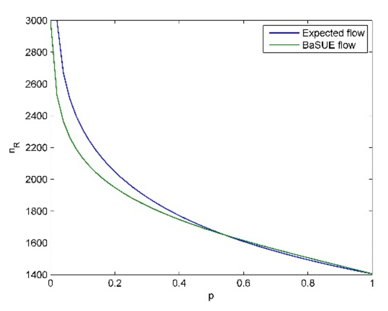
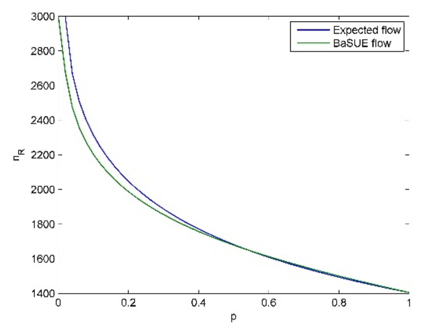
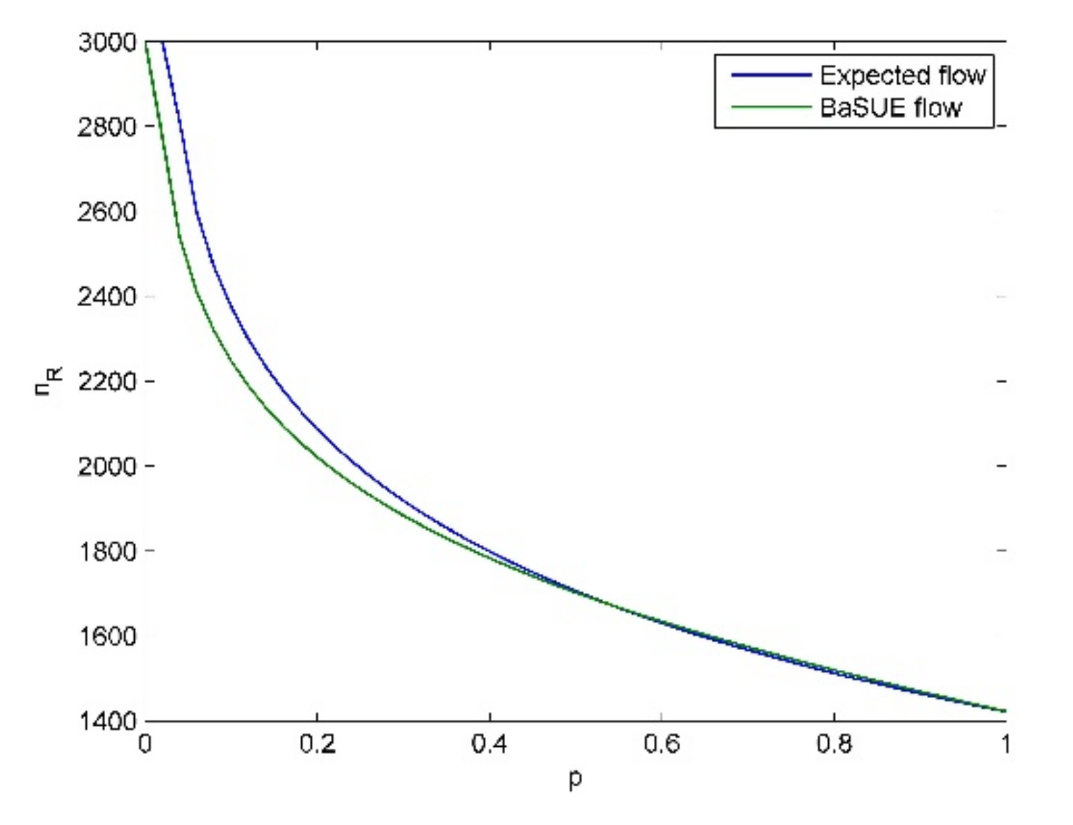
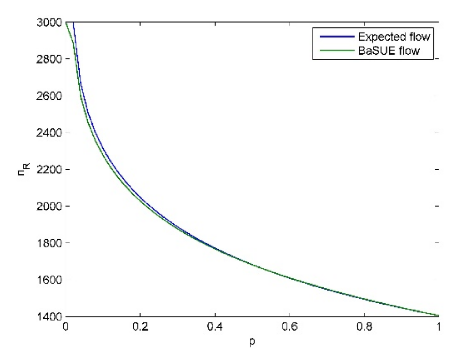
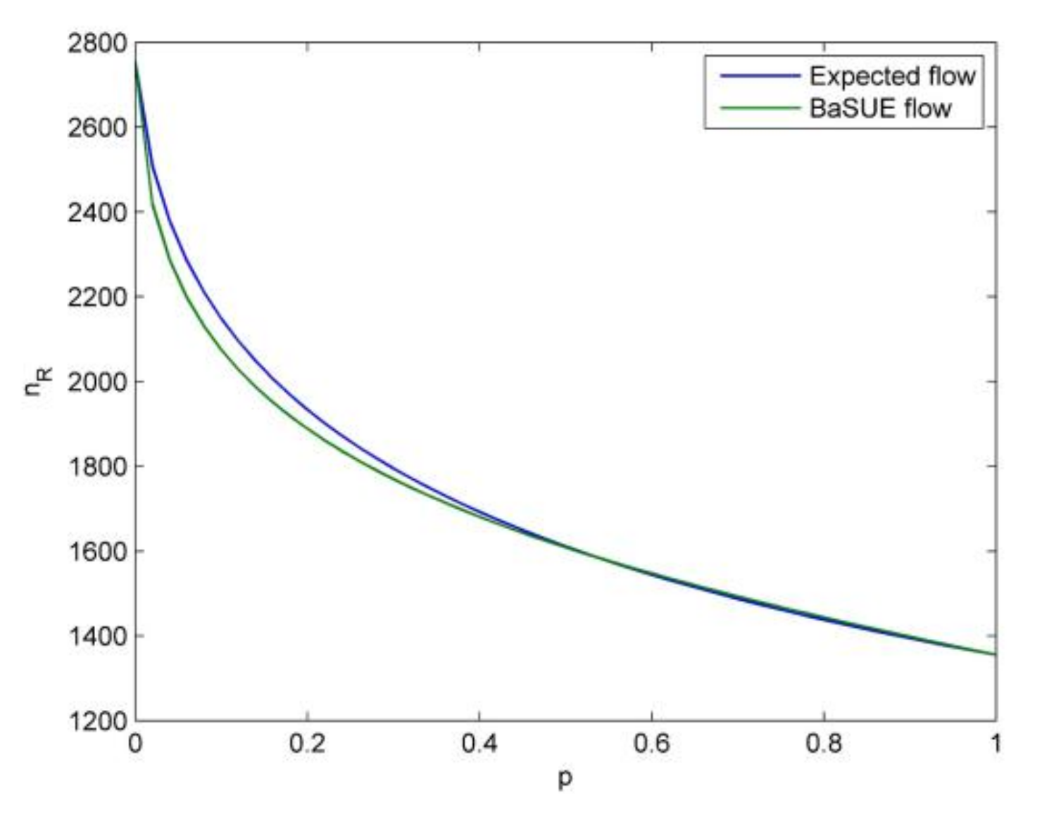
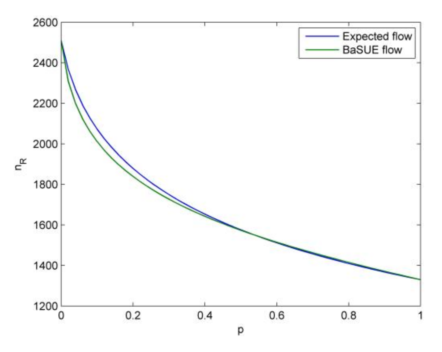
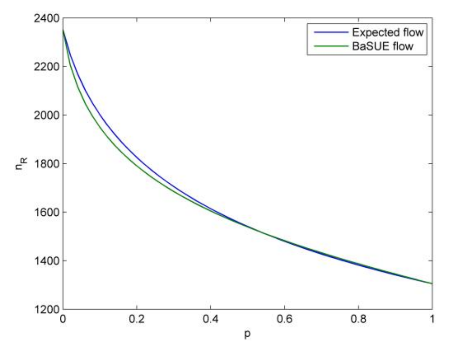
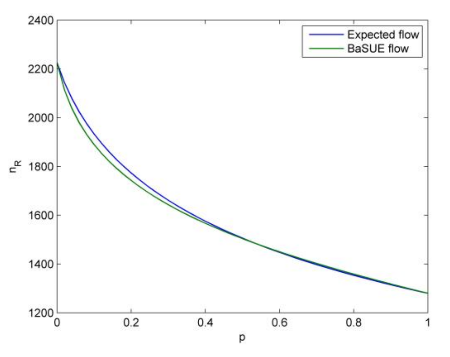
5.1. Case 1

In this case, $0\le \beta \left({\tau }_2-{\tau }_1\right)<p\left(t^{-}\left(N\right)-t_0\right)$ is satisfied. The travel cost on the risky option is 20, while the travel cost on the non-risky option is increased from 21 to 30 with the step size being 3. That is, we choose four representative values for travel cost on non-risky option. The salience bias $\delta$ is 0.3. The final equilibrium results are shown in

Table 1. Comparison of the equilibrium flow for representative values of $p\left({\tau }_1=20and{\tau }_2=21\right)$.

p	0.02	0.08	0.14	0.20	0.26	0.32	0.38	0.44	0.50
Expected flow	2627	2270	2093	1971	1878	1802	1738	1683	1635
BaSUE flow	2500	2177	2025	1921	1843	1778	1723	1675	1632
p	0.56	0.62	0.68	0.74	0.80	0.86	0.92	0.98	-
Expected flow	1592	1553	1518	1486	1456	1429	1403	1379	-
BaSUE flow	1593	1557	1524	1492	1463	1434	1407	1380	-

,

Table 2. Comparison of the equilibrium flow for representative values of $p\left({\tau }_1=20and{\tau }_2=24\right)$.

p	0.02	0.08	0.14	0.20	0.26	0.32	0.38	0.44	0.50
Expected flow	2923	2364	2162	2028	1927	1846	1779	1721	1670
BaSUE flow	2631	2247	2081	1971	1887	1820	1762	1721	1667
p	0.56	0.62	0.68	0.74	0.80	0.86	0.92	0.98	-
Expected flow	1625	1585	1548	1515	1484	1456	1429	1405	-
BaSUE flow	1627	1589	1554	1522	1491	1462	1433	1406	-

,

Table 3. Comparison of the equilibrium flow for representative values of $p\left({\tau }_1=20and{\tau }_2=27\right)$.

p	0.02	0.08	0.14	0.20	0.26	0.32	0.38	0.44	0.50
Expected flow	3000	2469	2234	2081	1978	1892	1820	1759	1706
BaSUE flow	2775	2318	2138	2021	1933	1861	1801	1749	1702
p	0.56	0.62	0.68	0.74	0.80	0.86	0.92	0.98	-
Expected flow	1659	1617	1579	1544	1512	1483	1455	1430	-
BaSUE flow	1660	1621	1585	1551	1519	1489	1460	1431	-

and

Table 4. Comparison of the equilibrium flow for representative values of $p\left({\tau }_1=20and{\tau }_2=30\right)$.

p	0.02	0.08	0.14	0.20	0.26	0.32	0.38	0.44	0.50
Expected flow	3000	2587	2310	2147	2029	1937	1862	1797	1742
BaSUE flow	2923	2391	2196	2071	1978	1903	1840	1786	1737
p	0.56	0.62	0.68	0.74	0.80	0.86	0.92	0.98	-
Expected flow	1692	1649	1609	1573	1540	1510	1481	1455	-
BaSUE flow	1694	1653	1616	1581	1548	1516	1486	1456	-

(here we select 17 representative values for p) and Figure 6, Figure 7, Figure 8 and Figure 9.

Before we discuss the main insights of the results, we present four common aspects in all the testings. (1) In our testing, the sufficient condition ${\sigma }_1\left(N\right)<{\sigma }_2\left(N\right)$ is satisfied, i.e., the relationship between ${\sigma }_1$ and ${\sigma }_2$ are shown in the upper-left figure of Figure 4. One can modify the travel utility func-tions to test other two situations; (2) In all the following figures, we claim that the cross point (denoted by $n_R^e$) of the two curves, the curve for expected flow following the principle of expected utility theory and the curve for BaSUE flow following the principle of flow-dependent salience theory, is a special situation, where travelers are risk-neutral according to Theorem (1). The condition, that the solution to the flow-dependent mode choice function and the solution to the equation ${\sigma }_1\left(n_R\right)<{\sigma }_2\left(n_R\right)$ coincide, needs to be satisfied, which can be verified by the related definitions. The above condition can also be used to figure out the $\tilde{P}$ of the bad state when travelers are risk-neutral. (3) When $p=0$ or $p=1$,we obtain the degeneration values for the equilibrium solution. In both cases, when $p=0$, the solution is obtained by solving the equation $u^{+}\left(n_R\right)=u^{NR}\left(N-n_R\right)$, and when $p=1$, the solution is obtained by solving the equation $u^{-}\left(n_R\right)=u^{NR}\left(N-n_R\right)$, given the specific values of ${\tau }_1$ and ${\tau }_2$. (4) In all the testings, we can always find the unique BaSUE solution, which demonstrates Proposition (3).

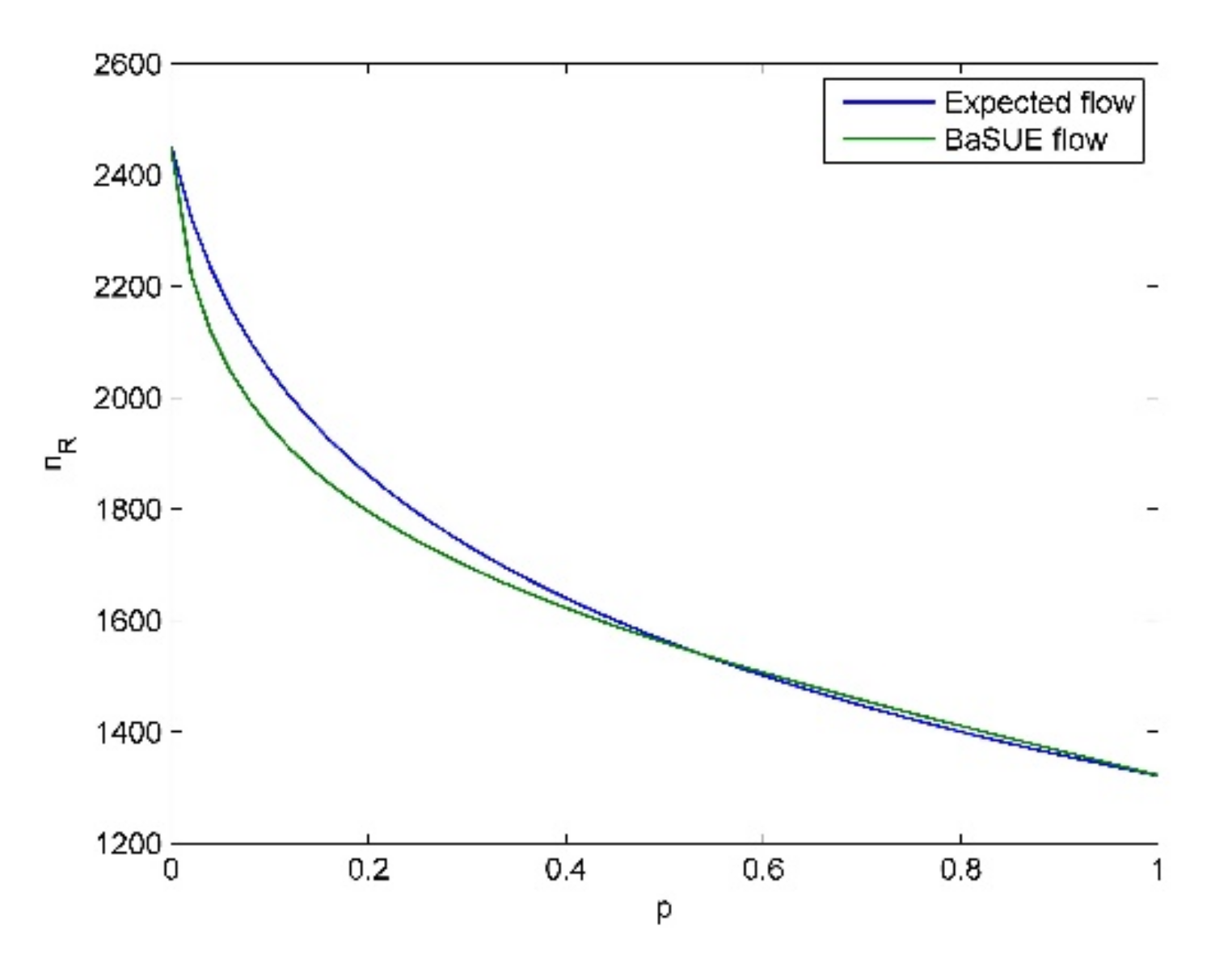
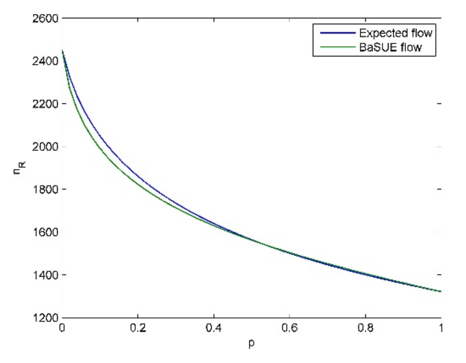
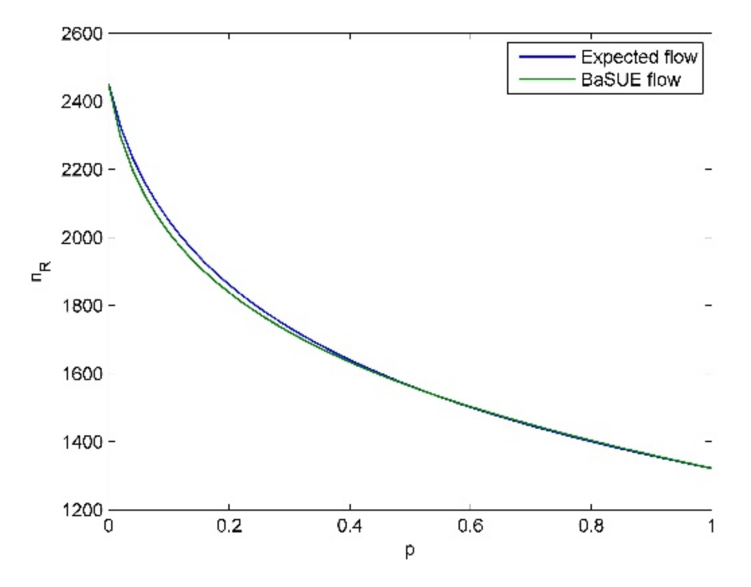
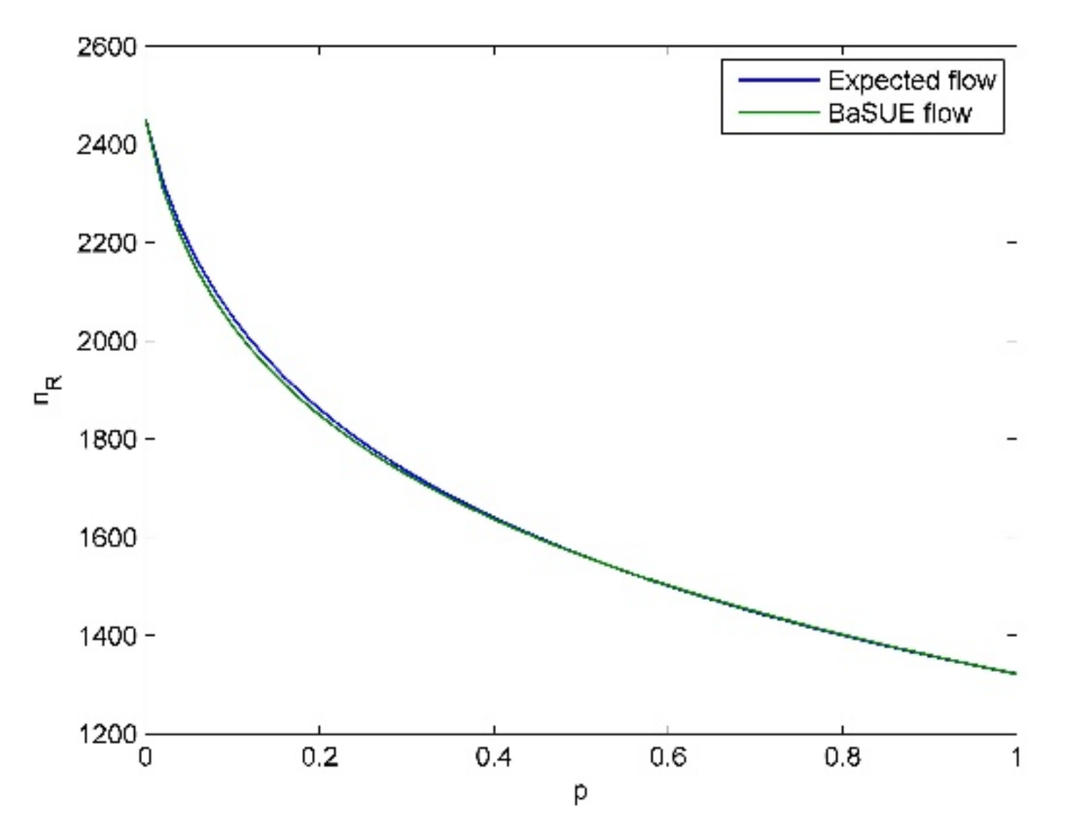
From these tables and figures, we see the following insights.

(1)

Given a specific objective probability (e.g., $p=0.2$), when the cost difference (cost difference here means ${\tau }_2-{\tau }_1$) become larger and larger, traffic flow on the risky option will become larger and larger, and vice versa. The intuitive explanation for this is that the increase of travel cost on non-risky option will make travelers choose the risky option.

(2)

When the probability of bad state is not large (e.g., $p=0.2$), travelers are risk-averse, and when the probability of bad state is relatively large (e.g., $p=0.7$), travelers are risk-seeking. We also see the cross point and its corresponding $\tilde{p}$, where travelers are risk-neutral as discussed before. For $p\in \left(0,\tilde{p}\right)$, travelers are risk averse, and for $p\in \left(\tilde{p},1\right)$, travelers are risk-seeking. These results seem to be non-intuitive, and it seems that if the travelers know that the risky option is in bad state (in good state) with high probability, they should choose the non-risky (risky) option, i.e., they should be risk-averse (risk-seeking). However, travelers’ salience characteristic means they put their attention on the unusual aspect. That is, if the risky option is in bad state (in good state) with high probability, considering the low (high) flow on the risky option (see Figure 6, Figure 7, Figure 8 and Figure 9), the good state (the bad state) is the unusual aspect according to our travel utility functions. Moreover, we can combine the results in Proposition (7) to present more interpretation on these phenomena. When the probability of bad state is not large, the equilibrium solution $n_{\mathrm{Re}}$ is larger than $n_R^c$, and thus, we know bad state is salient according to Proposition (7). In contrast, we know good state is salient when the probability of bad state is large. Therefore, we see these phenomena in the testings. All the above discussions also demonstrate the validity of Theorem (1).

(3)

When the cost difference become larger and larger, the extent of travelers’ risk-averse attitude becomes stronger almost, except when $p$ is very small, e.g., $p=0.02$. This is because larger cost difference will make travelers choose the risky option, which further makes the difference between travel utility of risky option in good state and the travel utility of non-risky option become smaller, considering the high flow on the risky option (see Figure 6, Figure 7, Figure 8 and Figure 9). Therefore, the bad state is more salient, which leads to the stronger extent of travelers’ risk-averse attitude. However, there is almost no difference between the risk-neutral equilibrium flow, i.e., the expected flow, and the risk-seeking equilibrium flow, i.e., the BaSUE flow when $p$ is relatively large. That is, travelers’ risk-seeking attitude following the flow-dependent salience theory has almost no effect on the equilibrium flow, compared to the results of expected utility theory. This is because the flow on the risky option is not large (see Figure 6, Figure 7, Figure 8 and Figure 9), which make the difference between the utilities on risky and non-risky option small.

(4)

With the increase of cost difference, we clearly see the corner equilibrium following the principle of expected utility theory. Meanwhile, larger cost difference means more situations with corner equilibrium. However, there is no corner equilibrium for BaSUE even though we increase the cost difference, which demonstrate Proposition (5).

Next, we fix the travel cost on the risky option (${\tau }_1=20$) and non-risky option (${\tau }_1=25$), and change the values of salience bias $\delta$. We choose four representative values for $\delta$, which are 0.1, 0.3, 0.5 and 0.7. $\delta =0.1$ implies that travelers have stronger salience bias, while $\delta =0.7$ implies the salience bias is weaker. The final equilibrium results are shown in Figure 10, Figure 11, Figure 12 and Figure 13. From these figures, we see the following insights. (1) With the increase of the value for $\delta$, the extent of travelers’ risk-averse attitude and risk-seeking attitude become weaker, and vice versa. (2) The value of $\delta$ has no effect on the cross point, where travelers are risk-neutral, as discussed before. (3) We clearly see the values for $p$, where there exists the corner equilibrium for expected flow, and the value of $\delta$ has no effect on this. (4) Even though travelers have very strong salience bias, e.g., $\delta =0.1$, the effect of travelers’ risk-seeking attitude following the flow-dependent salience theory on the equilibrium results can be ignored, compared to the results of expected utility theory. We can present similar explanations as the above testing.

5.2. Case 2

In this case, $-\left[t^{NR}\left(N\right)-t_0\right]<\beta \left({\tau }_2-{\tau }_1\right)<0$ is satisfied. The travel cost on the non-risky option is 20, while the cost on the risky option is increased from 21 to 30 with the step size being 3. That is, we choose four representative values for travel cost on risky option. The salience bias $\delta$ is also 0.3. The final equilibrium results are shown in

Table 5. Comparison of the equilibrium flow for representative values of $p\left({\tau }_1=21and{\tau }_2=20\right)$.

p	0.02	0.08	0.14	0.20	0.26	0.32	0.38	0.44	0.50
Expected flow	2509	2211	2048	1934	1845	1772	1711	1658	1611
BaSUE flow	2419	2130	1987	1888	1813	1750	1697	1650	1609
p	0.56	0.62	0.68	0.74	0.80	0.86	0.92	0.98	-
Expected flow	1570	1532	1498	1467	1438	1411	1386	1363	-
BaSUE flow	1571	1536	1503	1473	1444	1416	1389	1364	-

,

Table 6. Comparison of the equilibrium flow for representative values of $p\left({\tau }_1=24and{\tau }_2=20\right)$.

p	0.02	0.08	0.14	0.20	0.26	0.32	0.38	0.44	0.50
Expected flow	2367	2127	1984	1879	1797	1729	1671	1620	1576
BaSUE flow	2308	2062	1931	1839	1768	1709	1658	1614	1574
p	0.56	0.62	0.68	0.74	0.80	0.86	0.92	0.98	-
Expected flow	1536	1500	1468	1437	1410	1384	1360	1337	-
BaSUE flow	1537	1504	1473	1443	1415	1389	1363	1338	-

,

Table 7. Comparison of the equilibrium flow for representative values of $p\left({\tau }_1=27and{\tau }_2=20\right)$.

p	0.02	0.08	0.14	0.20	0.26	0.32	0.38	0.44	0.50
Expected flow	2248	2049	1921	1825	1749	1685	1631	1583	1541
BaSUE flow	2207	1995	1876	1790	1723	1667	1619	1577	1539
p	0.56	0.62	0.68	0.74	0.80	0.86	0.92	0.98	-
Expected flow	1503	1469	1437	1408	1382	1357	1334	1312	-
BaSUE flow	1504	1472	1442	1414	1387	1361	1337	1313	-

and

Table 8. Comparison of the equilibrium flow for representative values of $p\left({\tau }_1=30and{\tau }_2=20\right)$.

p	0.02	0.08	0.14	0.20	0.26	0.32	0.38	0.44	0.50
Expected flow	2144	1976	1861	1773	1702	1642	1591	1546	1506
BaSUE flow	2114	1931	1822	1742	1679	1626	1581	1540	1504
p	0.56	0.62	0.68	0.74	0.80	0.86	0.92	0.98	-
Expected flow	1470	1437	1407	1379	1354	1330	1308	1287	-
BaSUE flow	1471	1440	1411	1384	1359	1334	1310	1288	-

(here we also select 17 representative values for $p$) and Figure 14, Figure 15, Figure 16 and Figure 17.

From these tables and figures, we see the following insights. (1) Given a specific value of objective probability (e.g., $p=0.2$), when the cost difference (cost difference here means ${\tau }_1-{\tau }_2$) becomes larger and larger, traffic flow on the risky option will become smaller and smaller, and vice versa. The intuitive explanation for this is that the increase of travel cost on risky option will make travelers choose the non-risky option. (2) We also see travelers’ risk-seeking and risk-averse attitudes for different objective probability $ps$, and can give similar explanations as those in Case 1. Also, the risk-neutral attitude is a special condition. (3) When the cost difference become larger and larger, the extent of travelers’ risk-averse attitude almost remains the same, even though it becomes weaker. Increase in the cost difference will make more travelers choose non-risky option, and the difference between the utility of the risky option in good state and the utility of the non-risky option become larger. Meanwhile, increase of the value of ${\tau }_1$ makes this difference become smaller. Therefore, this difference remains almost the same, and we see this phenomenon on travelers’ risk-averse attitude. Similarly, there is almost no difference between the expected flow, and the BaSUE flow when travelers’ are risk-seeking, and we can present similar explanation as those in Case 1. (4) In this test, there is no corner equilibrium for both principles, and one can modify the travel utility functions and travel costs to show the corner equilibrium.

Next, we fix the travel cost on the risky option (${\tau }_1=25$) and non-risky option (${\tau }_2=20$), and change the values of salience bias $\delta$. We also choose four different value for $\delta$, which are 0.1, 0.3, 0.5 and 0.7. The final equilibrium results are shown in Figure 18, Figure 19, Figure 20 and Figure 21. From these figures, we see the similar behavioral insights as the tests shown from Figure 10, Figure 11, Figure 12 and Figure 13.

6. Conclusions

In this paper, we discussed travelers’ bi-attribute (travel time and travel cost) risky mode choice behavior with one risky option (e.g., the highway) and one non-risky option (e.g., the transit), and provided new insights to this kind of behavior. We proposed to use the flow-dependent salience theory to support this research aim, and developed the bi-attribute salient travel utility model. Furthermore, we examined the long-run effect of this model and developed the bi-attribute salient user equilibrium model, which can partially remedy the unrealistic behavioral assumptions used in the classical Wardropian user equilibrium principle. We theoretically proved the existence and unique of the equilibrium, and based on the equilibrium results, we analyzed the travelers’ risk attitudes on the bi-attribute mode choice problem. Finally, we run the numerical examples to show the sensitivity of the equilibrium results to the input parameters, which are cost difference and salience bias.

The novelty of our paper is to study the effect of travelers’ salience characteristic on the bi-attribute mode choice behavior. Salience here is context-dependent, and travelers’ attention is drawn to the bi-attribute salient travel utility. The main findings of this paper are summarized as follows. (1) Travelers’ attitude can be risk-averse, risk seeking or risk-neutral in the bi-attribute mode choice problem. If the objective probability of bad state $p$ is relatively small, travelers are risk-averse, and if $p$ is relatively large, travelers are risk-seeking. Only in the special situation, where the solution to the flow-dependent mode choice function and the solution to the equation ${\sigma }_1\left(n_R\right)={\sigma }_2\left(n_R\right)$ coincide, travelers are risk-neutral. This condition can also be used to figure out the $p$ of the bad state when travelers are risk-neutral, which can further be used to figure out the $ps$ for risk-averse attitude and the $ps$ for risk-seeking attitude. (2) The extent of travelers’ risk-averse and risk-seeking attitudes can be affected by their salience bias and the cost difference, while their risk-neutral attitude is only affected by the cost difference. (3) If the travel cost on the risky option is smaller than that on the non-risky option, we see that the extent of travelers’ risk-averse attitude becomes stronger with the increase of the cost difference, while if the travel cost on the non-risky is smaller, we see that the extent of travelers’ risk-averse attitude almost remains the same with the change of cost difference. In both cases, we find that the effect of travelers’ risk-seeking attitude can be ignored, which is identical to the effect of their risk-neutral attitude almost, even though travelers’ salience bias is very strong. (4) The cost difference is closely related to the corner equilibrium, and travelers’ salience characteristic can affect the occurrence of the corner equilibrium. (5) The relationship between the salience functions can be affected by the travel cost, and we identify the sufficient conditions for this (see the sufficient condition (17)).

Our findings can provide implications for the policy design and implementation, especially on the congestion tolling and transit fare design, which are summarized as follows. (1) The salience characteristic can cause non-intuitive risk attitudes for travelers, which needs to be considered in the policy design and implementation. (2) The policy makers can use the congestion tolling and transit fare design (focusing on the cost difference) to change travelers’ risk attitudes, and further change the distribution of the traffic flow. Especially, the change on travelers’ risk-averse attitude is effective. (3) If the policy makers focus on the corner equilibrium, the effect of travelers’ salience characteristic is notable, which can change the effect of cost difference. (4) The policy makers can also use the congestion tolling and transit fare design to change the relationship between the salience functions, focusing on our sufficient conditions.

There are several directions which merit further study. Firstly, in this paper, we only focus on the effect of travel cost on the equilibrium, and, in the future, we will discuss the optimal congestion tolling and transit fare design problem considering the salience characteristic, where the results of our paper can serve as the basis. Secondly, there is perception error for travelers, and in further research we will discuss the effect of perceived objective probability. Thirdly, our method can also be used for the two-route equilibrium analysis, but an extension to the multiple options is needed for the analysis on the general traffic network. Finally, a behavioral experiment can be conducted to estimate the key parameters in our method, i.e., the salience bias, as discussed in the introduction.