COVID-19 and Financial Sustainability of Academic Institutions

Abstract

The COVID-19 pandemic has had a significant impact on higher education. Steering academic institutions through the pandemic is a complex and multifaceted task that can be supported with model-based scenario analysis. This article studies the short-term and long-term effects of the pandemic on the financial health of a college using scenario analysis and stress testing with a system dynamics model of a representative tuition-dependent college. We find that different combinations of the pandemic mitigation protocols have varying effects on the financial sustainability of an academic institution. By simulating six individual components of the COVID-19 shock, we learn that due to the causal complexity, nonlinear responses and delays in the system, the negative shocks can propagate widely through the college, sometimes with considerable delays and disproportionate effects. Scenario analysis shows that some pandemic mitigation choices may destabilize even financially healthy institutions. The article concludes that higher education needs new sustainable business models.

1. Introduction

The COVID-19 pandemic has had a tremendous effect on the higher education sector. When COVID-19 hit the global economy in Spring 2020, academic institutions responded to the health emergency in several ways [1], including switching from in-person classes to online instruction, implementing health and safety measures such as installing plastic shields and sanitizing equipment, and testing for COVID-19. Burdened by significant financial losses, some colleges have cut faculty and staff positions [2]. The chosen approaches to pandemic mitigation depend on the success measures that colleges follow, their values and their operating constraints such as the size of their endowment [3]. Several observers predicted that colleges would struggle financially and many would perish [4].

Higher education is a significant contributor to the U.S. economic competitiveness and growth [5], but the sector faces a multitude of challenges and existential threats, such as the decline of enrollments due to demographic reasons [6]. The COVID-19 crisis posits another existential challenge. However, there is a lack of rigorous research aimed at explaining the effects of the pandemic on the financial health of a university. This article aims to fill this research gap.

The goal of this article is to study the short-term and long-term effects of the pandemic on the financial condition of a representative college using scenario analysis and stress testing with a simulation model. We demonstrate how scenario analysis and stress testing using computational models can assist with the complex task of steering a campus through the pandemic by helping to identify effective and financially sustainable pandemic mitigation approaches.

We use the college model [6,7], which simulates operations of a typical private not-for-profit tuition-based college. The model represents a college as a complex service system [8,9,10,11,12,13] that consists of interconnected economic agents and elements such as students, faculty, facilities, and financial variables. The model is implemented using the system dynamics methodology [14,15,16]. To evaluate the financial vulnerability of an academic institution to the COVID-19 shock, we adopt the market risk framework and the Market Stress Test Score (MSTS) that have been developed by Zemsky et al. [17] specifically for the purpose of stress-testing in higher education. When integrated with data and decision support systems used by colleges and universities, the approach developed in this article can help academic leaders make informed institutional planning and policy decisions.

Our main research questions are the following: What are the major effects of a pandemic such as COVID-19 on the financial sustainability of a university? Under what conditions and responses does the university remain financial sustainable in the short-term and in the longer term? We find that due to the causal complexity, nonlinear responses and delays in the system, the negative shocks due to COVID-19 can propagate widely through the college, sometimes manifesting themselves with considerable delays and disproportionate effects. Breaking the COVID-19 shock into six components and simulating their impact on the college reveals that while in isolation each stressor is not likely to undermine the college, certain combinations of the shocks may destabilize even financially healthy institutions. These simulations explain why, despite extraordinary financial and operational challenges, only very few colleges have closed during the pandemic [18]. The simulations also suggest that some colleges may succumb to the negative effects of COVID-19 long after the pandemic is officially over.

Below, we discuss related literature and describe the methods employed in this article. Then, we explain how we separate the pandemic-related market risk into components, which is followed by the results, discussion, and conclusion sections.

2. Related Literature

This article is related to the literature on model-informed academic management and the management of the pandemic-related risk on campus.

2.1. Model-Informed Academic Management

Model-based scenario analysis is not widely used in academic planning, even though early attempts to use computational models in academic decision-making date back to the 1960s [19,20]. Higher education resource planning and management are complex tasks that involve multiple stakeholders [9,11,21] within academic institutions, which are highly interconnected and non-linear systems [9,22,23,24,25]. Simulations are tools for evaluating alternative strategies and scenarios before committing resources to a strategy [26]. As data should not drive but rather inform decision making [27], models should not drive decisions but rather be part of a process that recognizes the importance of the human judgement as one of the inputs. By design, models are imperfect and incomplete because of the numerous assumptions that must be made during model construction. Model-informed decision making, as opposed to model-driven decision making, takes into account organizational values and campus politics that models may exclude.

2.2. Models That Evaluate Pandemic Mitigation on Campus

Simulation models have been used to evaluate the cost-effectiveness of the pandemic mitigation approaches on campus. Wildman et al. [3] created a simulation-based decision support system for evaluating policies aimed at containing the COVID-19 pandemic at an academic institution. The authors offer a detailed analysis of the impact of various policy combinations on health outcomes using an agent-based epidemiological model that can be calibrated to specific universities. Agents represent students, faculty and staff that are in contact with each other via a static network. The probabilities of infections are represented by the weights of the links between agents. University policies and interventions including social distancing, tracing, quarantining, closing gyms, and teaching remotely modify the probabilities of infection, which are recorded by adjusting link weights. Simulations identify policies that lead to optimal outcomes such as the least number of infections. Their analysis suggests, for instance, that it is more cost-effective to test frequently a select group of student-facing staff than increasing frequency of testing for the entire campus.

Losina et al. [28] also conduct sensitivity analysis of alternative COVID-19 mitigation approaches on campus using simulations. They contrast clinical outcomes and costs. The model is based on the susceptible–infected–recovered (SIR) infection model in which the population transitions between the SIR states with probabilities that are dependent on estimated contact-hours and infectivity rates. The authors estimate, for example, that wearing masks and social distancing can reduce campus cases of infections by 87 percent at the cost of $170 per case. If the college is willing to engage in routine testing, which would cost anywhere between $2000 and $17,000 per person, 96 percent of infections can be eliminated.

3. Methods and Model

The article uses the system dynamics method.

3.1. System Dynamics

System dynamics is a stock-and-flow consistent methodology for modeling problems that include complex causality, feedback, and delays [14,15,16,29]. System dynamics models are well suited for higher education planning and budgeting at the institutional level [9,10,23,30,31,32,33]. Invented in the late 1950s for the analysis of management problems [34], system dynamics has been applied in many areas (e.g., [29,32,35,36,37,38]), and it is a popular modeling approach in operations research [39]. Mathematically, system dynamics models are continuous-time nonlinear and non-stochastic sets of integral equations that are solved numerically. System dynamics is taught worldwide [40,41,42,43].

3.2. The College Model

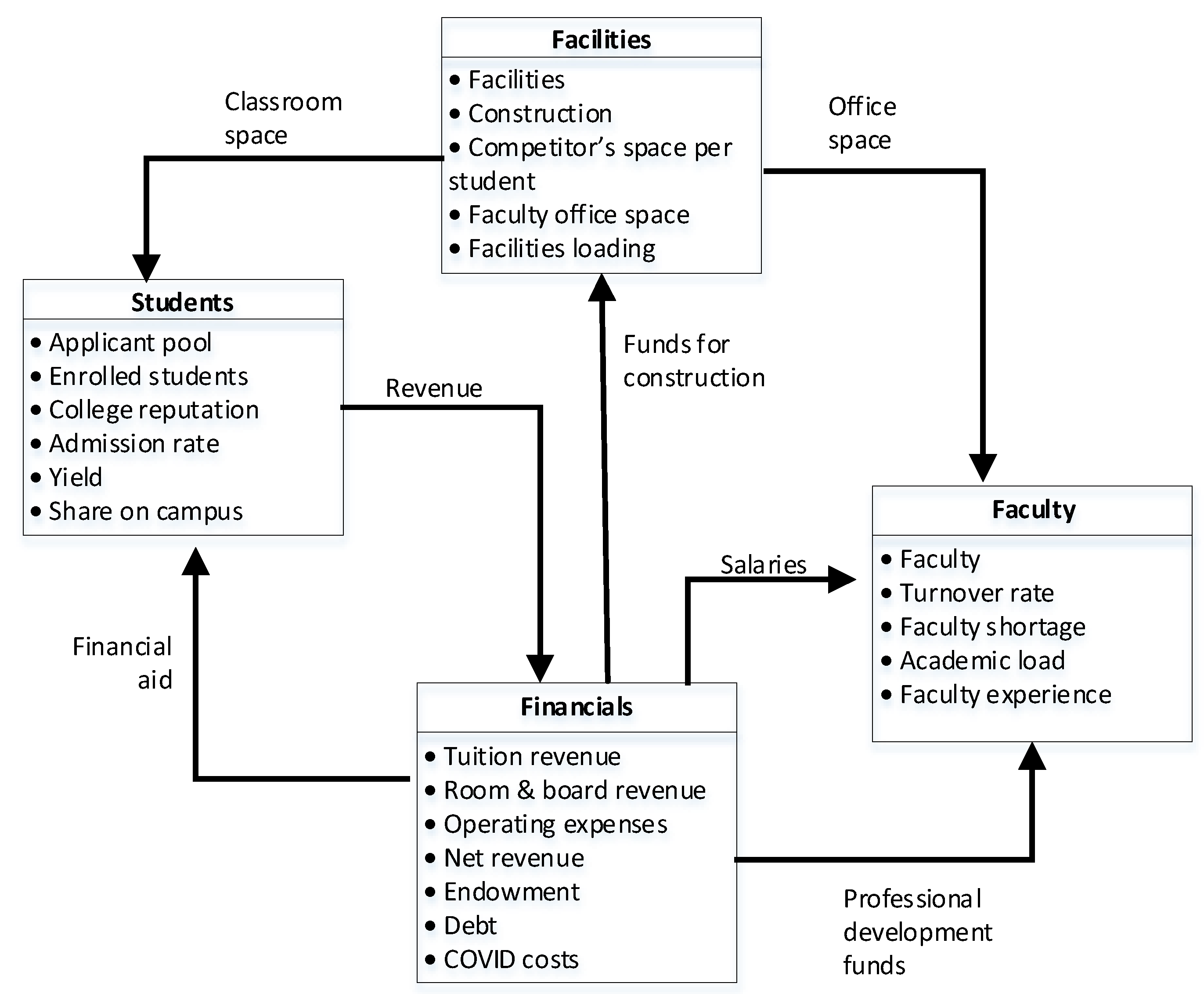
This analysis uses a system dynamics computational model of a stylized four-year private not-for-profit college. A detailed description of the model can be found in Pavlov and Katsamakas [6]. The model consists of four interconnected modules: students, faculty, facilities, and financials (Figure 1). The model has been built in consultations with campus stakeholders [44] and its formulation is consistent with the economic theory of academic institutions (e.g., [9]). The model has been implemented using the system dynamics modeling software Stella Architect that is available from isee systems.

The model assumes that before the pandemic, the college is in a financially healthy steady state. The tuition discount rate is assumed to be 40 percent, which implies that full-paying students subsidize those who receive financial aid. The student retention rate is set to 95 percent, which is a typical number for top-rated private institutions [45]. In the steady state, the return on endowment funds and the annual endowment draw are equal and set to 5 percent, which is within the range of the 5-year average return for endowments and accepted practices for endowment spending [46]. Even though only about 13 percent of all academic institutions have no debt [47], for the sake of simplicity, our model assumes that the simulated college is debt-free before the pandemic. The model also assumes that the college has enough liquid assets (i.e., cash and cash equivalents) to cover one year of operations.

3.3. Stress Testing Academic Institutions

Stress testing is an important yet rare practice in higher education [48]. Zemsky et al. [17] developed the Market Stress Test Score (MSTS) that tracks four variables: the first-year enrollments, retention of students, market price, and endowment-to-operating-expense ratio (EOER). The market price is defined as the revenue from tuition, room, and board less the financial aid divided by the number of students.

Table 1. Market stress test score (MSTS) calculation.

Component	Value is Less than the Alert Level	Value is Less than the Warning Level	Trend is Negative and Absolute Value is Greater than 1 Percent
First-year enrollment	+1	+1	+1
Retention	+1	+1	+1
Market price	+1	+1	+1
Endowment-to-expense ratio	+1	+1	+1

explains that the MSTS is calculated by increasing the score when the components drop below thresholds or exhibits strong negative trends. Thresholds are referred to as “alerts” and “warnings” and set to 20 and 10 percentile values of the peer group. For this analysis, we set alerts to 80 percent and warnings to 70 percent of the steady state values. When a component drops below the alert level, the MSTS is increased by 1. If the component drops even further, below the warning value, the MSTS increases by 1 again. If the variable exhibits a negative trend greater than one percent, a 1 is added to the MSTS. The trend m for variable x is calculated according to the following equations:

$$m=\frac{x-\overline{x}}{\overline{x}{t}_m}$$

$$\overline{x}=x_0+\underset{}{\overset{}{{\displaystyle \int }}}\frac{x-\overline{x}}{t_m}dt$$

Here $\overline{x}$is the first order exponential average of $x$, $t_m$ is the averaging time and $x_0$ is the initial value of variable $x$. We set $t_m=3$ years and $x_0$ is the steady state value. The risk score for each component is between 0 and 3. Therefore, since the MSTS has four components, its range is between 0 and 12. In the steady state, the MSTS is 0, but the higher the financial risk that the institution faces, the higher the score. According to Zemsky et al. [17] (p. 95), any institution with the MSTS above 4 faces a substantial market risk.

4. Pandemic-Related Risks

Complex dynamic problems can be studied by disaggregating them into components that are examined individually [49]. In this study, we consider six components of the COVID-19 shock, which we call stressors S1 through S6. Figure 2 shows their impact on a college. An upward pointing red arrow indicates that this particular variable increases due to COVID-19, and a downward pointing red arrow means that the value of the variable is likely to decrease due to COVID-19. A positive link between two variables signifies a positive causality between them. Negative causalities are shown with negative links.

Below, we describe the six stressors that are studied in this article.

S1.

Fewer students on campus: Due to social distancing concerns, about 10 percent of campuses completely suspended campus operations as a mitigation response to COVID-19 and about 4 percent continued to teach in person [50]. Other colleges offered hybrid instruction [50]. Since fewer students live on campus, the revenue from room and board decreases.

S2.

Lower enrollments: The economic and health crisis caused by COVID-19 led to a decline in student enrollments. In the U.S., in the Fall 2020, the undergraduate enrollment was 4 percent lower than the previous year and enrollment of the first-time students dropped by 16 percent [51]. Some students deferred admission. For example, at Harvard, 349 out of 895 admitted students deferred their admission in the Fall 2020 [52]. This trend may continue, as the number of Common Applications at the end of 2020 was 2 percent lower than at the same time the previous year [52]. Moreover, by the end of November 2020, the number of people who filled out the Free Application for Federal Student Aid, or FAFSA, fell by 17 percent from the previous year, suggesting that many less-affluent students do not plan to attend college in the following academic year [53]. Therefore, the tuition revenue and revenue from room and board may decline.

S3.

COVID-19 preparedness of the campus: Colleges had to prepare campuses for operating in the pandemic environment. They posted signs, created disinfectant stations, installed separators, changed HVAC, and established sites for COVID-19 testing. These fixed costs added to the operating expenses.

S4.

Health and safety measures: According to the recent survey by The American College Health Association [50], 84 percent of colleges and universities that responded to the survey are testing for COVID-19. Nearly all in this group test symptomatic students, but only some test asymptomatic students. Of those who do surveillance testing, 59 percent do it at least once a week. The rest do it every other week, monthly or several times a semester. The primary indicated reasons for not conducting testing more frequently were lack of human resources and cost of testing.

S5.

Greater financial need: The pandemic worsened the economic situation in the U.S. Therefore, families may not be able to contribute the same amounts toward education, which may increase requests for financial aid (e.g., [54]). Since student decisions depend on the financial aid, to stay competitive colleges must offer better tuition discounts [13,21]. Greater amounts of financial aid decrease the net tuition revenue and net revenue from room and board.

S6.

Calls to reduce tuition: There is a perception among students and parents that if courses are not taught in person, the tuition should be lower. For example, students at Columbia University have demanded a reduction of sticker price by 10 percent and an increase in financial aid by the same amount [54]. Reducing tuition directly impacts in a negative way the net tuition revenue. Among about 30 institutions that have cut tuition over the years prior to the pandemic, the results have been mixed [17].

5. Computational Experiments and Results

This section first examines one stressor at a time and then combines six stressors together. All simulations start in the steady state in year 0 (noted in graphs as YR0). The pandemic starts in year 4 (YR4 in graphs) and ends in year 6 (YR6). Results for each of the simulation sets are presented in a table and two figures. The table includes short and long-term values for key indicators. We define short-term as the time during the pandemic and the long-term is about 10 years out. The tables can be thought of as snapshots of the state of the college. Each column in the table shows a scenario, including the steady state. We color code some values as green, yellow, and red, which stand for good, concern, and danger. The figures show how the college experiences the pandemic over time. For each stressor, one figure shows trajectories of key variables, and the second figure displays changes of the stress score.

5.1. S1: Fewer Students Live on Campus

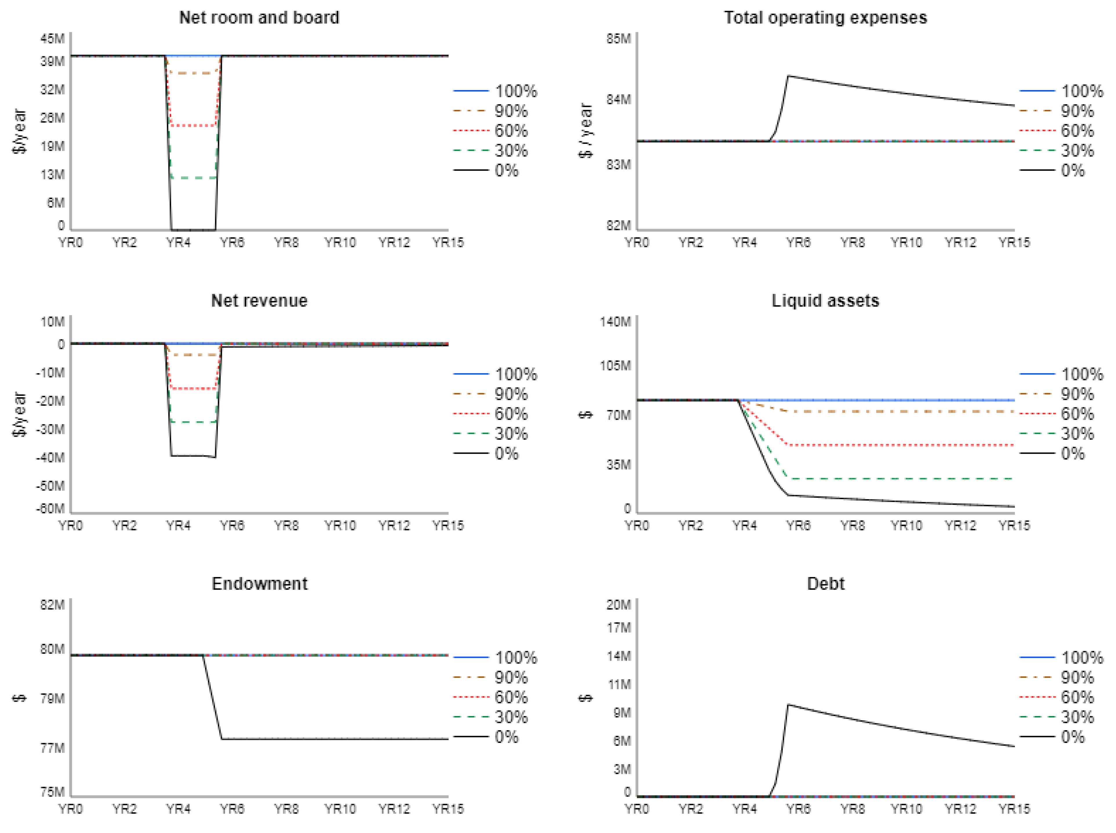
When fewer students live on campus, it affects negatively the room and board revenue. As a simplification, we assume that before the pandemic, 100 percent of students lived on campus, which is the base case. We simulate four scenarios when 90, 60, 30, and 0 percent of students remain on campus. Simulations show (see

Table 2. The effect of fewer students on campus (S1). M = millions. K = thousands.

	Indicators (Units)	Share of Students on Campus, %
		100	90	60	30	0
Short-term (YR5)	Incoming class (students)	600	600	600	600	600
	Students on campus (students)	2204	1984	1322	661	0
	Net room and board ($/year)	40 M	36 M	24 M	12 M	0 M
	Total operating expenses ($/year)	83 M	83 M	83 M	83 M	83 M
	Net revenue ($/year)	0	−4 M	−16 M	−28 M	−40 M
	Liquid assets ($)	80 M	76 M	64 M	52 M	40 M
	Endowment ($)	80 M	80 M	80 M	80 M	80 M
	Debt ($)	0	0	0	0	0
	Market Stress Test Score	0	1	2	3	3
Long-term (YR13)	Incoming class (students)	600	600	600	600	600
	Students on campus (students)	2204	2204	2204	2204	2204
	Net room and board ($/year)	40 M	40 M	40 M	40 M	40 M
	Total operating expenses ($/year)	83 M	83 M	83 M	83 M	83 M
	Net revenue ($/year)	0	0	0	0	−768 K
	Liquid assets ($)	80 M	72 M	48 M	24 M	6 M
	Endowment ($)	80 M	80 M	80 M	80 M	77 M
	Debt ($)	0	0	0	0	6 M
	Market Stress Test Score	0	0	0	0	0

and Figure 3 and Figure 4) that in the short term, between years 4 and 6, the revenue drops substantially in each of the scenarios. In the worst scenario (0 percent of students remain on campus), after year 5, total operating expenses increase because the college has to borrow for operations and servicing debt is costly (see Figure 3).

After the pandemic is over in year 6, revenue returns to the pre-pandemic level, which ensures that the college can balance its books (see Figure 3). However, the financial position of the college is not as strong as before the pandemic. Its liquid assets are at a lower level (Figure 3) which makes the college vulnerable to future external shocks. The endowment is not affected except in the worst case (Figure 3) when no students remain on campus. Then, the college needs to make emergency withdrawals from the endowment and borrow for operations, which results in the post-pandemic debt (see Figure 3 and last column in Table 2).

After the pandemic, to restore its financial health, the college needs to replenish the emergency stock of liquid assets (see long-term values in Table 2) either by increasing revenue to above the pre-pandemic levels or cutting cost that would allow it to run surpluses. Revenue can also be increased through tuition hikes or fundraising.

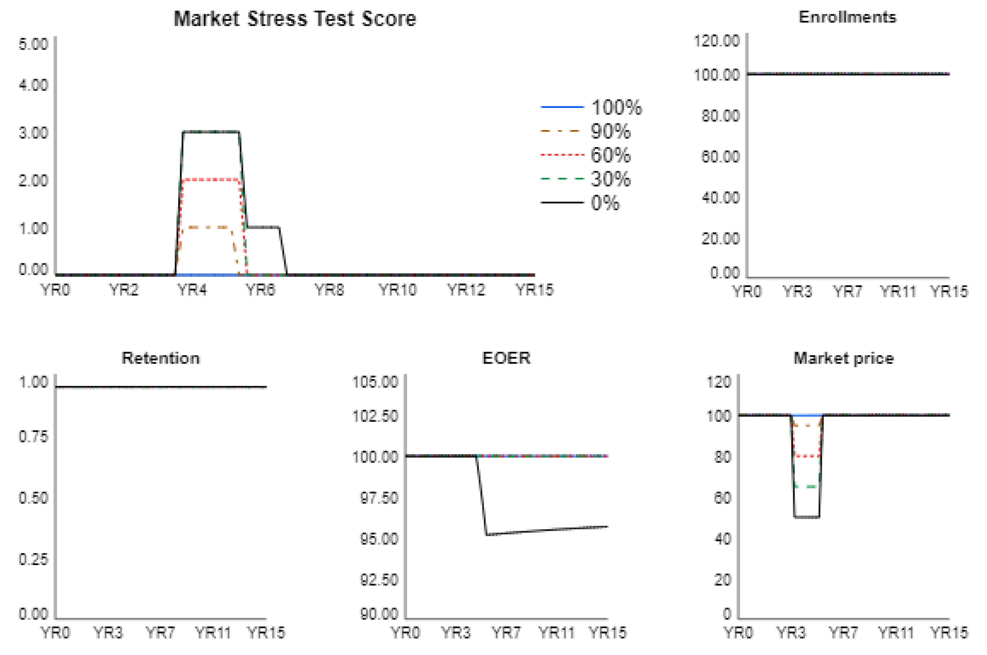
The values of the Market Stress Test Score in Table 2 show that the score quite adequately captures situations when the financial status of the college is worsening. Figure 4 decomposes the market stress test score into its components. When there are fewer students on campus, room and board revenue declines causing the market price to drop. The market price is the net revenue (total revenue from tuition, room, and board less the financial aid) divided by the number of students. The market price recovers once students return to campus. Because the college has to make emergency withdrawals from the endowment and borrow for operations when no students are allowed on campus, the EOER fraction drops during the pandemic, and then, it stays low. Following the rules for calculating the stress test score outlined in Table 1, the MSTS index increases during the pandemic, but it is always below 4.

5.2. S2: Enrollment Decline

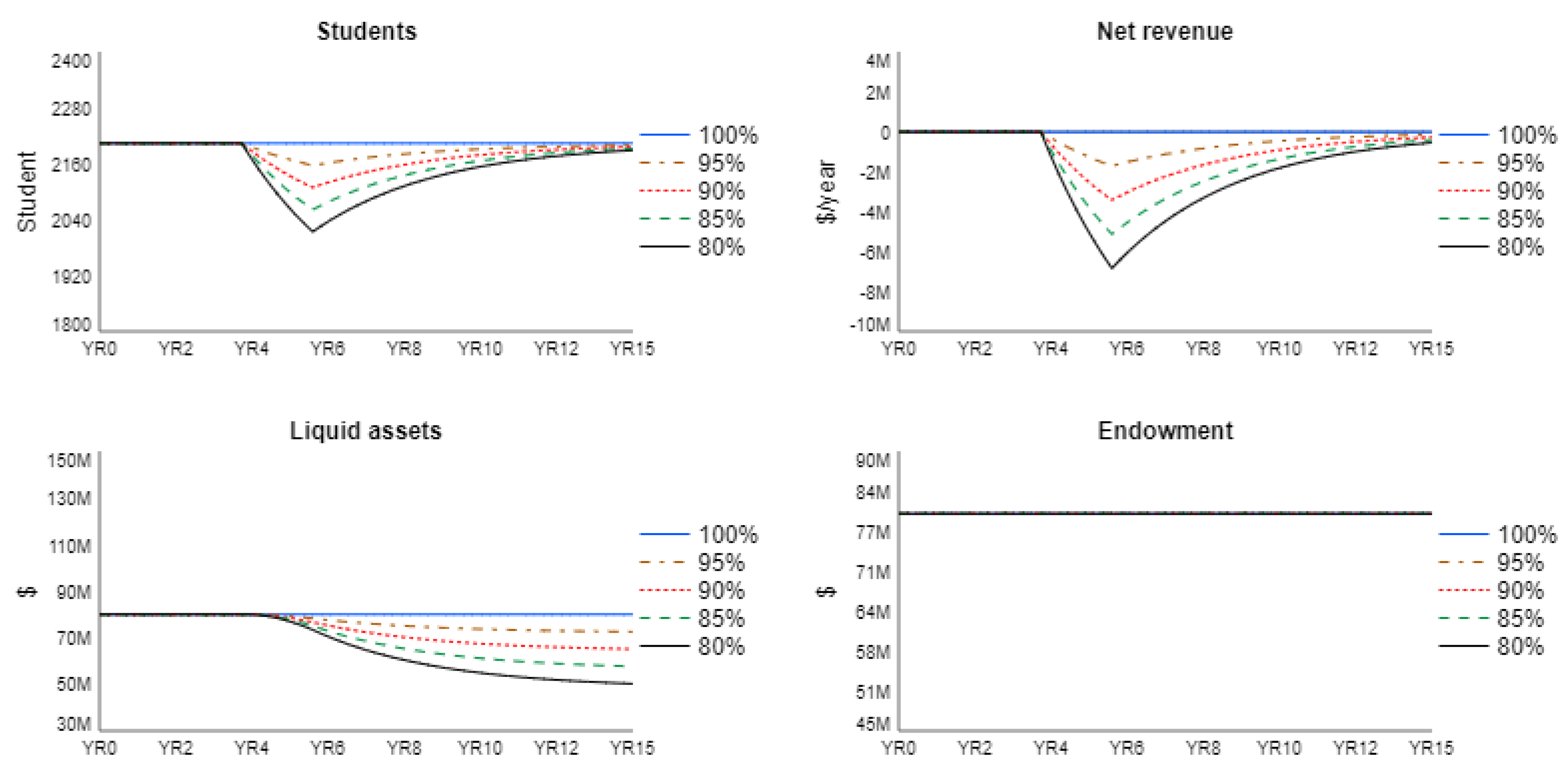
We simulate a case when only a fraction of a typical incoming class of students enroll during the pandemic. The base case is compared to the scenarios when 95, 90, 85, and 80 percent of a regular class enroll. The drop in enrollments during the pandemic leads to fewer students taking courses, less revenue from room and board and negative net revenue, i.e., a deficit (see short-term values in

Table 3. The effect of enrollment decline (S2). M = millions. K = thousands.

	Indicators (Units)	Fraction of Incoming Class, %
		100	95	90	85	80
Short-term (YR5)	Incoming class (students)	600	570	540	510	480
	Students on campus (students)	2204	2177	2150	2123	2096
	Net room and board ($/year)	40 M	39 M	39 M	38 M	38 M
	Total operating expenses ($/year)	83 M	83 M	83 M	83 M	83 M
	Net revenue ($/year)	0	−1 M	−2 M	−3 M	−4 M
	Liquid assets ($)	80 M	79.6 M	79.2 M	78.8 M	78.4 M
	Endowment ($)	80 M	80 M	80 M	80 M	80 M
	Debt ($)	0	0	0	0	0
	Market Stress Test Score	0	1	1	1	2
Long-term (YR13)	Incoming class (students)	600	600	600	600	600
	Students on campus (students)	2204	2197	2191	2184	2177
	Net room and board ($/year)	40 M	40 M	39 M	39 M	39 M
	Total operating expenses ($/year)	83 M	83 M	83 M	83 M	83 M
	Net revenue ($/year)	0	−0.2 M	−0.5 M	−0.7 M	−1 M
	Liquid assets ($)	80 M	72.9 M	65.9 M	58.8 M	51.7 M
	Endowment ($)	80 M	80 M	80 M	80 M	80 M
	Debt ($)	0	0	0	0	0
	Market Stress Test Score	0	0	0	0	0

). The total operating expenses do not increase neither in the short term, nor the long term since the deficit is covered by the regular endowment draw and by using liquid assets (see Table 3).

Assuming that the incoming class bounces back to 600 as soon as the pandemic is over (see long-term values in Table 3), the college nearly recovers its revenue but still runs a small deficit in YR13 (see Table 3 and Figure 5). In the long term, liquid assets are still below the pre-pandemic level (see Table 3). Moreover, Figure 5 clearly shows that liquid assets are still declining even after the pandemic because cash and cash-equivalents are used to cover the deficit. The simulations suggest that the financial consequences of the pandemic will be felt by colleges long after the campuses reopen.

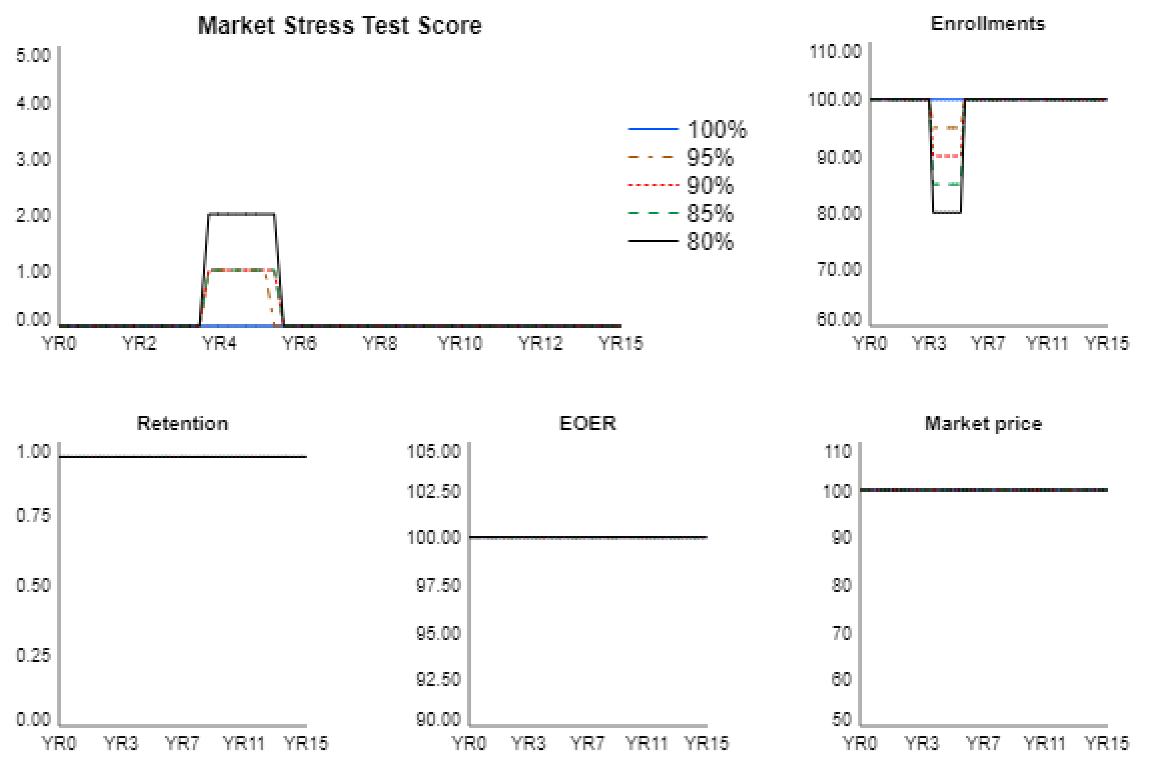
Table 3 summarizes the values of the market stress test score (MSTS) in the short and long term during different scenarios. The MSTS increases to 1 or 2 during the pandemic. The trajectories of its components in Figure 6 demonstrate that the MSTS increases due to the drop in enrollments. In the long-term, the MSTS is zero (Figure 6) because all contributing components are back to the steady state levels.

5.3. S3: COVID-19 Preparedness

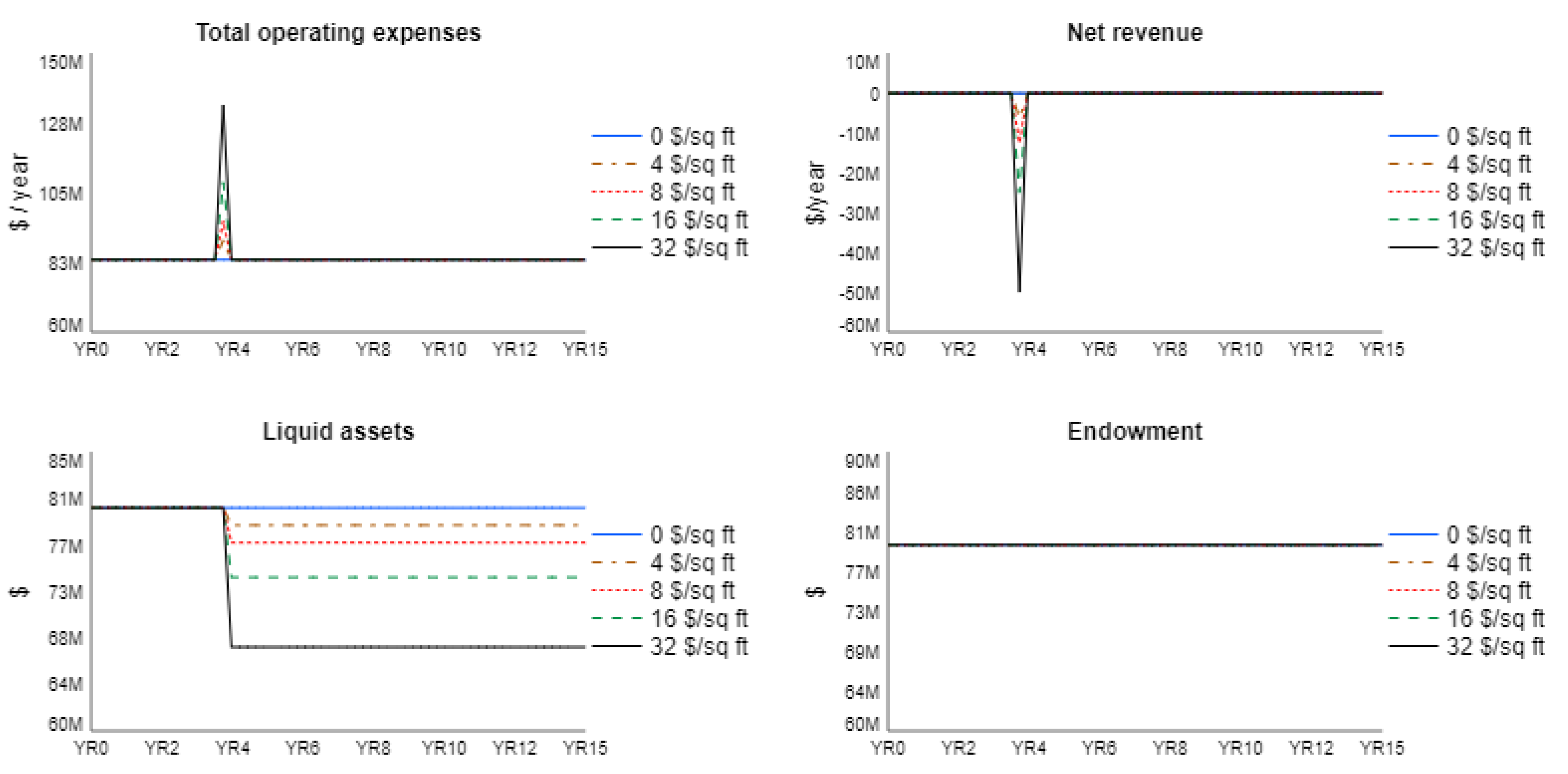
These scenarios simulate a one-time expense in YR4 by the college on COVID-19 preparedness measures such as posting the signs, purchasing disinfectant stations and separators, updating the HVAC, and establishing sites for COVID-19 testing. We assume that the cost of COVID-19 preparedness can be 4, 8, 16, or 32 $/sq ft, which is compared to the base case when the cost is 0 $/sq ft. The short-term and long-term results of the simulations are shown in

Table 4. The effect of COVID-19 preparedness (S3). M = millions. K = thousands.

	Indicators (Units)	Cost of Preparedness, $/sq ft
		0	4	8	16	32
Short-term (YR4)	Incoming class (students)	600	600	600	600	600
	Students on campus (students)	2204	2204	2204	2204	2204
	Net room and board ($/year)	40 M	40 M	40 M	40 M	40 M
	Total operating expenses ($/year)	83 M	89.6 M	95.8 M	108 M	133 M
	Net revenue ($/year)	0	−6.3 M	−12.5 M	−25 M	−50 M
	Liquid assets ($)	80 M	80 M	80 M	80 M	80 M
	Endowment ($)	80 M	80 M	80 M	80 M	80 M
	Debt ($)	0	0	0	0	0
	Market Stress Test Score	0	1	1	2	3
Long-term (YR13)	Incoming class (students)	600	600	600	600	600
	Students on campus (students)	2204	2204	2204	2204	2204
	Net room and board ($/year)	40 M	40 M	40 M	40 M	40 M
	Total operating expenses ($/year)	83 M	83 M	83 M	83 M	83 M
	Net revenue ($/year)	0	0	0	0	0
	Liquid assets ($)	80 M	78.4 M	76.9 M	73.8 M	67.5 M
	Endowment ($)	80 M	80 M	80 M	80 M	80 M
	Debt ($)	0	0	0	0	0
	Market Stress Test Score	0	0	0	0	0

, and Figure 7 includes trajectories of several key variables.

The one-time expense in year 4 immediately causes operating expenses to go up and puts net revenue into the red for each of the scenarios (see short-term effects in Table 4 and trajectories in Figure 7). The deficit (negative net revenue in Figure 7) is covered by using liquid assets (see liquid assets decline in Figure 7). Note that liquid assets drop and never recover to the pre-pandemic level. To address this issue, the college can increase revenue or cut operating expenses in order to create a surplus that can be saved as an emergency cash reserve. As clear from Table 4 and Figure 7, the endowment is not affected because the endowment withdrawals stay within the pre-pandemic range in all scenarios.

Since we assume that the COVID-19 preparedness is a one-time expense, the MSTS index is shaped as a spike (Figure 8). The spike is caused by the higher operating expenses in year 4 that leads to a spike in the EOER ratio. The other three components of the market stress test score stay constant. In all scenarios, the score is never above 3 (see Figure 8 and the short-term values in Table 4). In the long term, the stress score returns to the pre-pandemic level of zero, which accurately reflects that the college is back to being financially stable.

5.4. S4: Health and Safety Measures

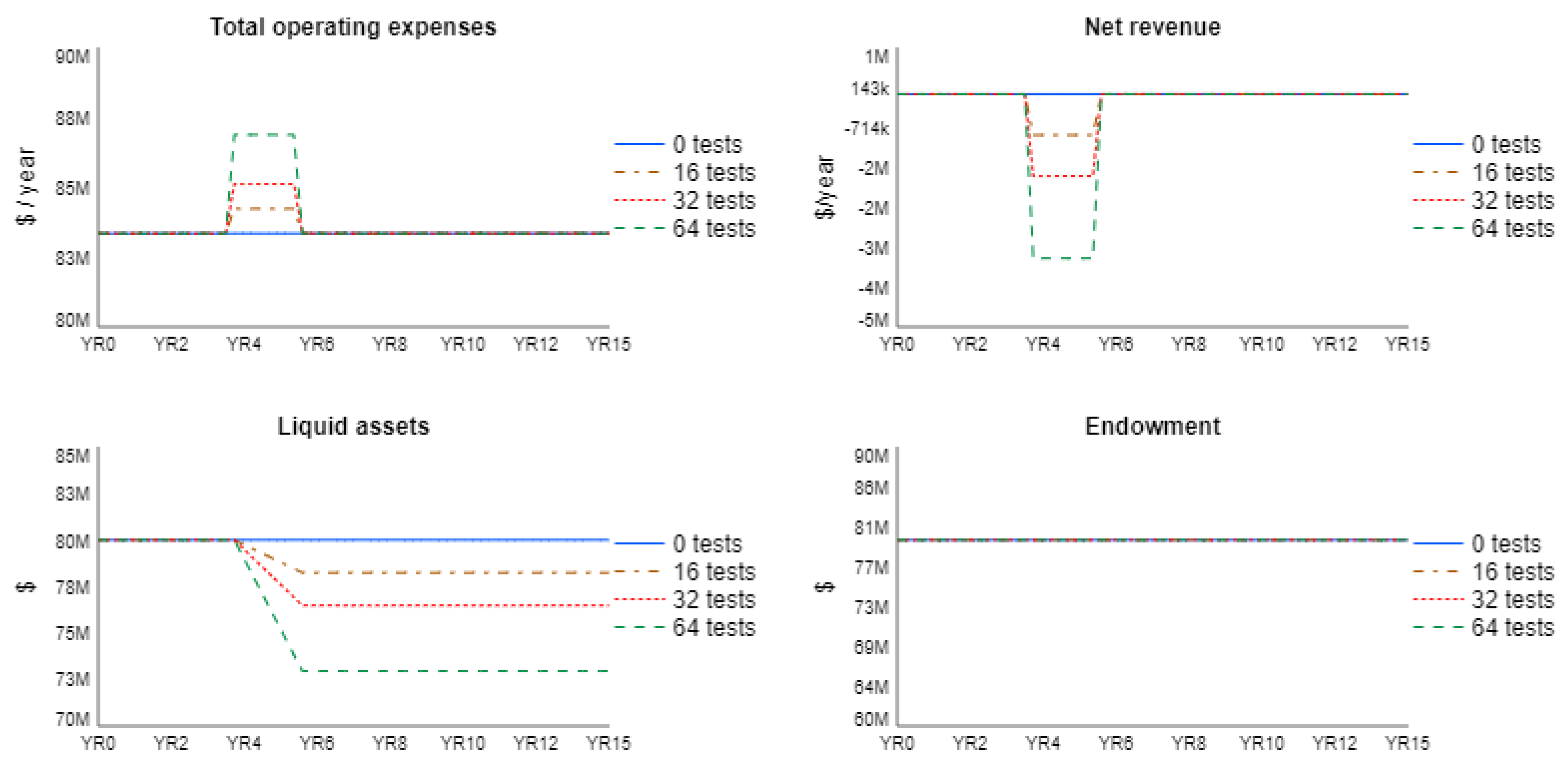
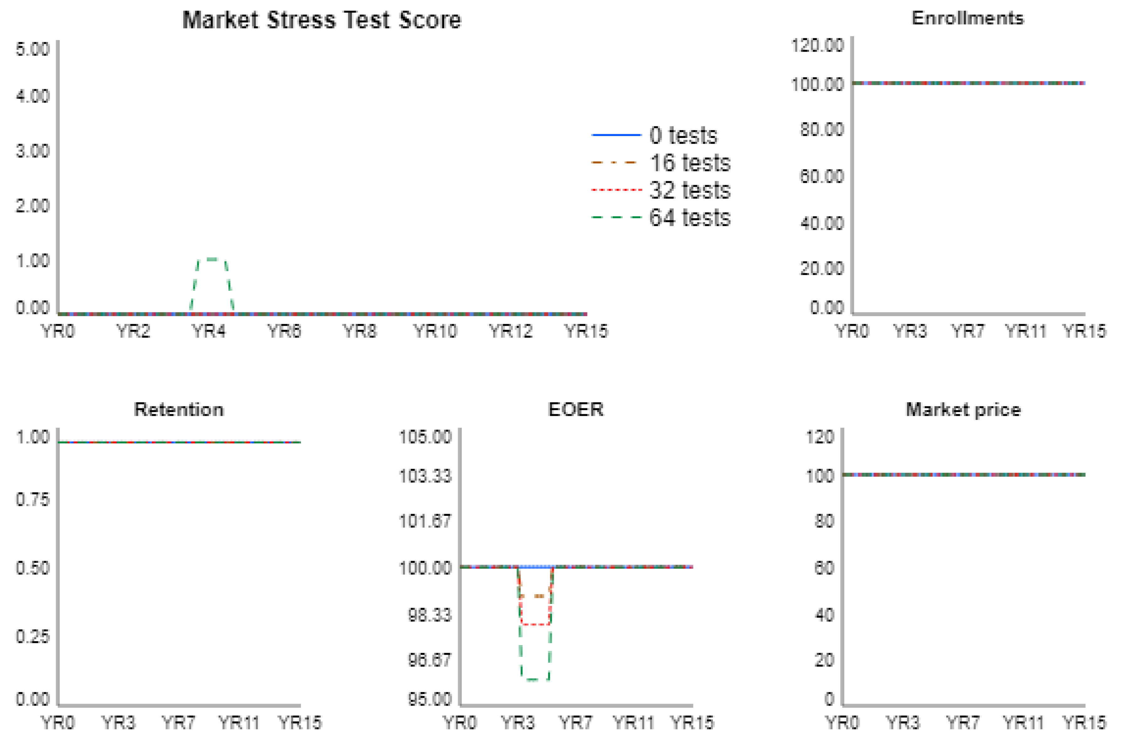
Here, we examine the impact of the recurring health and safety costs on the financial state of the college. We assume that all students are on campus and each of them is tested 16, 32, or 64 times a year at a fixed cost of $25/test. In the steady state, the students are not tested. Key indicators from each scenario form columns in

Table 5. The effect of health and safety measures (S4). M = millions. K = thousands.

	Indicators (Units)	COVID-19 Testing, Times/yr
		0	16	32	64
Short-term (YR4)	Incoming class (students)	600	600	600	600
	Students on campus (students)	2204	2204	2204	2204
	Net room and board ($/year)	40 M	40 M	40 M	40 M
	Total operating expenses ($/year)	83 M	84 M	85 M	87 M
	Net revenue ($/year)	0	−1 M	−1.8 M	−3.5
	Liquid assets ($)	80 M	79 M	78 M	76 M
	Endowment ($)	80 M	80 M	80 M	80 M
	Debt ($)	0	0	0	0
	Market Stress Test Score	0	0	0	1
Long-term (YR13)	Incoming class (students)	600	600	600	600
	Students on campus (students)	2204	2204	2204	2204
	Net room and board ($/year)	40 M	40 M	40 M	40 M
	Total operating expenses ($/year)	83 M	83 M	83 M	83 M
	Net revenue ($/year)	0	0	0	0
	Liquid assets ($)	80 M	78 M	76 M	73 M
	Endowment ($)	80 M	80 M	80 M	80 M
	Debt ($)	0	0	0	0
	Market Stress Test Score	0	0	0	0

. Figure 9 shows the trajectories of several important variables. The market stress test score is recorded in Figure 10.

As can be seen in the short-term section of Table 5 and in Figure 9, total operating expenses increase during the pandemic, which leads to negative net revenue. This deficit is covered from liquid assets and by making regular withdrawals from the endowment. Because the endowment withdrawals do not rise to the emergency levels, the endowment stays at the constant level in the short and long term. However, once reduced, the stock of liquid assets stays low. The college can improve its position with respect to the liquid assets only if it runs a surplus and saves the cash for the rainy day.

According to the levels of the market stress test score in Table 5, the college is never in a dangerous financial situation. In the short run, the MSTS index increases to 1 only in the most expensive scenario when students are tested 64 times a year (see last column in Table 5). As becomes clear from Figure 10, when it increases, the MSTS index rises due to the brief dip of the EOER ratio caused by the operating expenses temporarily increasing during the pandemic. The MSTS score never reaches the threshold of 4 that would sound an alarm. In the long term, the stress score is back to the pre-pandemic level (see Table 5 and Figure 10), which accurately indicates that the college is financially stable again.

5.5. S5: Financial Aid

This set of runs simulates an increase in financial aid. The simulations assume that the pre-pandemic steady state discount rate is 40 percent. Financial aid is assumed to increase one year after the start of the pandemic, i.e., in year 5, that pushes the discount rates to 45, 50, 55, and 60 percent. We assume that the discount rates stay at this level for the duration of the simulation. As can be seen in

Table 6. The effect of greater financial aid (S5). M = millions. K = thousands.

	Indicators (Units)	Tuition Discount Rate, %
		40	45	50	55	60
Short-term (YR5)	Incoming class (students)	600	600	600	600	600
	Students on campus (students)	2204	2204	2204	2204	2204
	Net room and board ($/year)	40 M	36 M	33 M	30 M	26 M
	Total operating expenses ($/year)	83 M	83 M	83 M	83 M	83 M
	Net revenue ($/year)	0	−6.6 M	−13.2 M	−19.8 M	−26.4 M
	Liquid assets ($)	80 M	80 M	80 M	80 M	80 M
	Endowment ($)	80 M	80 M	80 M	80 M	80 M
	Debt ($)	0	0	0	0	0
	Market Stress Test Score	0	1	1	2	3
Long-term (YR13)	Incoming class (students)	600	600	600	600	600
	Students on campus (students)	2204	2204	2204	2204	2204
	Net room and board ($/year)	40 M	36 M	33 M	30 M	26 M
	Total operating expenses ($/year)	83 M	83 M	85 M	91 M	97 M
	Net revenue ($/year)	0	−6.6 M	−15.6 M	−28 M	−40.8 M
	Liquid assets ($)	80 M	27.1 M	0.4 M	66 K	27 K
	Endowment ($)	80 M	80 M	70 M	63 M	60 M
	Debt ($)	0	0	17 M	69 M	126 M
	Market Stress Test Score	0	0	1	3	5

, the immediate result is that the net room and board revenue drops, more so the greater the discount rate. That leads to short-term decreases of net revenue in each scenario. This leads to the drop of the market price, which is a contributing factor for the MSTS indicator. In the short term, the MSTS score increases as high as 3 for the worst case when the discount rate is 60 percent.

In the long run, given that the discount rates do not change, the net room and board revenue stays at the same levels as during the pandemic (compare short and long-term numbers for net room and board in Table 6). To cover the deficit, the college draws from the endowment and the stock of liquid assets. However, as can be seen in Figure 11, for the cases when the discount rate is above 45 percent, the college also has to borrow for operations. Debt service adds to the total operating expenses (see numbers for total operating expenses in Figure 11 and Table 6). Long term, in the three worst cases, the liquid assets are nearly completely drained by year 13, and the endowment is also diminished (see long-term numbers in Table 6 and trajectories in Figure 11).

The MSTS increases due to the lower endowment, higher operating expenses and lower market price. As the EOER worsens through the simulations (see Figure 12), the stress score climbs up, with the highest numbers for the worst-case scenario when the tuition discount rate is 60 percent. The two components that are continuously driving the escalation of the MSTS index are the market price and the EOER ratio.

5.6. S6: Lower Tuition

Assuming that the college is initially in the steady state, here we simulate the scenarios when the college responds to the demands to lower tuition. We assume that once tuition is reduced, it stays at the same level. In this set of experiments, tuition is adjusted in year 5, one year after the pandemic starts, to $25,000, $20,000, $15,000, $10,000, while the steady state tuition prior to the pandemic is $30,000.

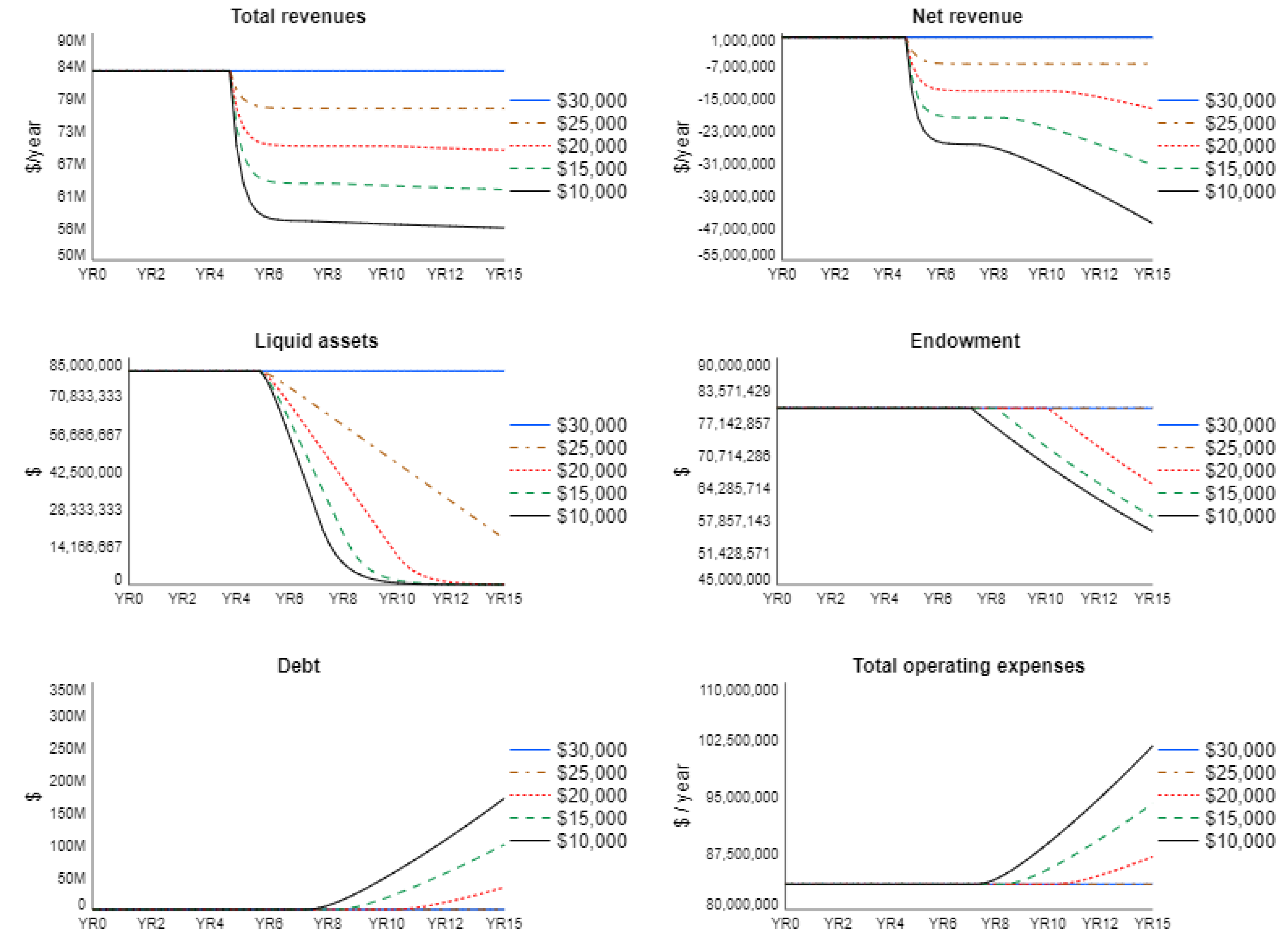
Lowering tuition immediately impacts net revenue, which is in the red in all scenarios (see the short-term section in

Table 7. The effect of lower tuition (S6). M = millions. K = thousands.

	Indicators (Units)	Tuition, $
		30 K	25 K	20 K	15 K	10 K
Short-term (YR6)	Incoming class (students)	600	600	600	600	600
	Students on campus (students)	2204	2204	2204	2204	2204
	Net room and board ($/year)	40 M	40 M	40 M	40 M	40 M
	Total operating expenses ($/year)	83 M	83 M	83 M	83 M	83 M
	Net revenue ($/year)	0	−6 M	−12.4 M	−18.6 M	−24.8 M
	Liquid assets ($)	80 M	76.5 M	73 M	69.5 M	66 M
	Endowment ($)	80 M	80 M	80 M	80 M	80 M
	Debt ($)	0	0	0	0	0
	Market Stress Test Score	0	0	0	0	0
Long-term (YR13)	Incoming class (students)	600	600	600	600	600
	Students on campus (students)	2204	2204	2204	2204	2204
	Net room and board ($/year)	40 M	40 M	40 M	40 M	40 M
	Total operating expenses ($/year)	83 M	83 M	84.7 M	89.6 M	95.2 M
	Net revenue ($/year)	0	−6.6 M	−15 M	−26.9 M	−39.3 M
	Liquid assets ($)	80 M	30.4 M	794 K	117 K	49 K
	Endowment ($)	80 M	80 M	71.7 M	64.6 M	61.4 M
	Debt ($)	0	0	12 M	59 M	111 M
	Market Stress Test Score	0	0	1	3	6

). The college is forced to dip into the liquid assets that drop in the short term (see the short-term section in Table 7). Liquid assets are lower when the tuition is lower. The college, however, does not need to conduct emergency withdrawals from the endowment or incur debt for operations. Therefore, in the short-term, the endowment stays constant at $80 M (see Table 7). The MSTS index stays in the green in the short run in each of the scenarios (see Table 7); this is appropriate since the college is still financially sustainable even though it runs deficits in each scenario.

In the long term, the net revenue is negative (see the long-term section of Table 7), which is caused by the fact that tuition revenue is reduced while the total operating expenses go up due to the higher leverage and the accompanying debt servicing payments. The debt and total operating expenses are the highest when the tuition is reduced to $10,000 (see Table 7 and Figure 13). Combined with the reduced endowment ($61.4 M in the long term), high total operating expenses contribute to the MSTS index increasing to the alarming level of 6.

The dynamic can be traced in Figure 13. The total revenue drops in each scenario as compared to the base run when the tuition is $30,000. Net revenue also drops nonlinearly as total operating expenses increase due to more leveraged position of the college. The college has no choice but to borrow for operations since its depleted liquid assets and the endowment are insufficient to support the deficit in the longer run.

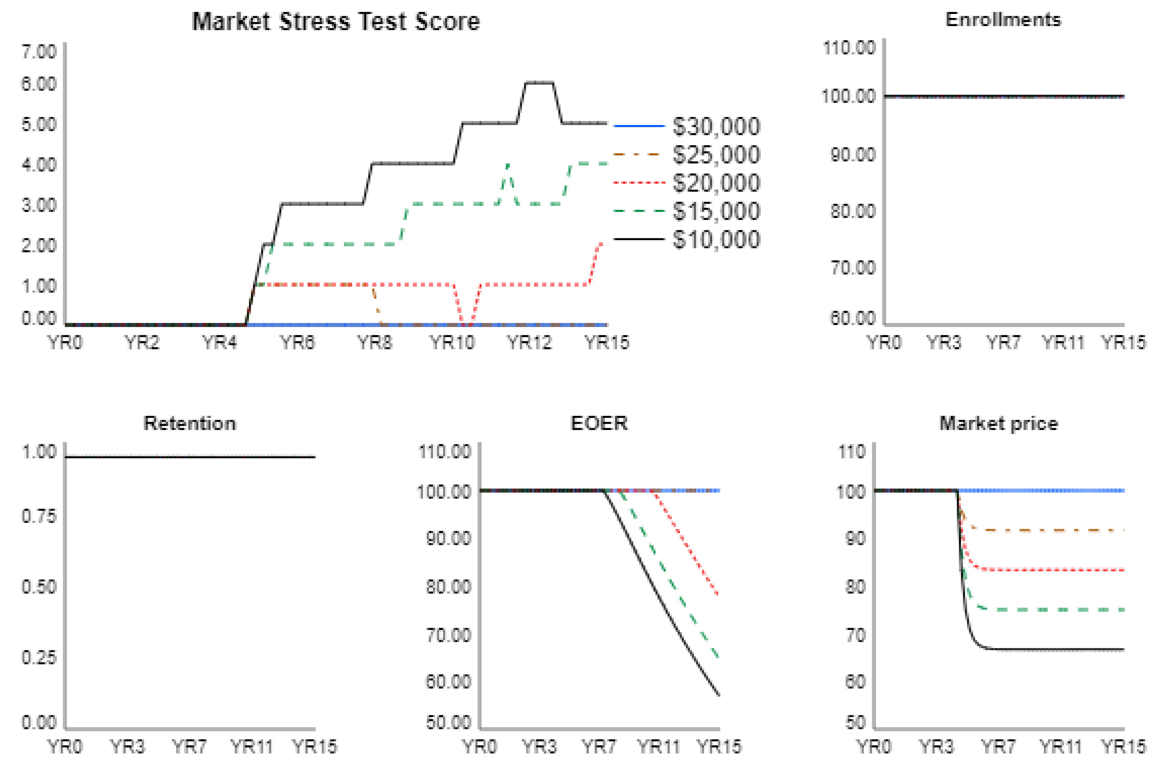
Confirming short-term data in Table 7, Figure 14 shows that the MSTS index stays within the acceptable range of less than 4 during the pandemic. However, it gradually climbs up through the duration of the simulations and in the worst case, when tuition is $10,000, the MSTS index peaks at 6, which is above the threshold value of 4 suggested by Zemsky et al. [17]. The index increases due to the decline of the market price and the EOER ratio (see Figure 14), which are the components of the MSTS index.

5.7. Combined Stressors

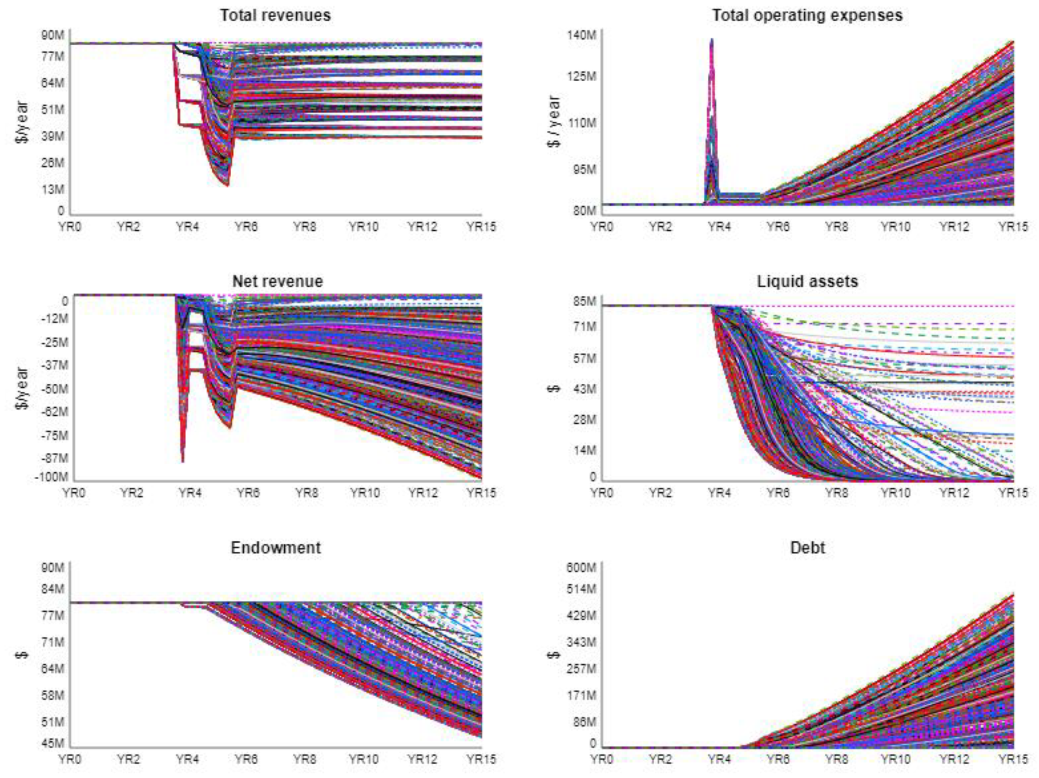
To test the combined effect of all six stressors occurring simultaneously, we conduct 1000 runs for different combinations of parameter values from within the ranges specified above for simulations S1–S6. The parameter values are picked using the Latin Hypercube sampling method. Figure 15 shows the results of the sensitivity run; the figure shows the ranges of possible outcomes. For example, we can see that the total revenue drops at the beginning of the pandemic and recovers somewhat after the pandemic is over. The total operating expenses spike during the pandemic, which may lead to significant budget deficits, i.e., negative net revenue. The financial shortages are covered by drawing on liquid assets, the endowment funds and by borrowing, when needed. In neither of the scenarios the endowment is completely depleted even in the long run. However, the debt may increase by the factor of five compared to the total revenue in the steady state; note that the college is assumed to have no debt at the beginning of the simulation. The dynamic story in Figure 15 suggests that some campus decisions aimed at mitigating the pandemic may lead to long-term consequences that are worse than the immediate effects during the pandemic.

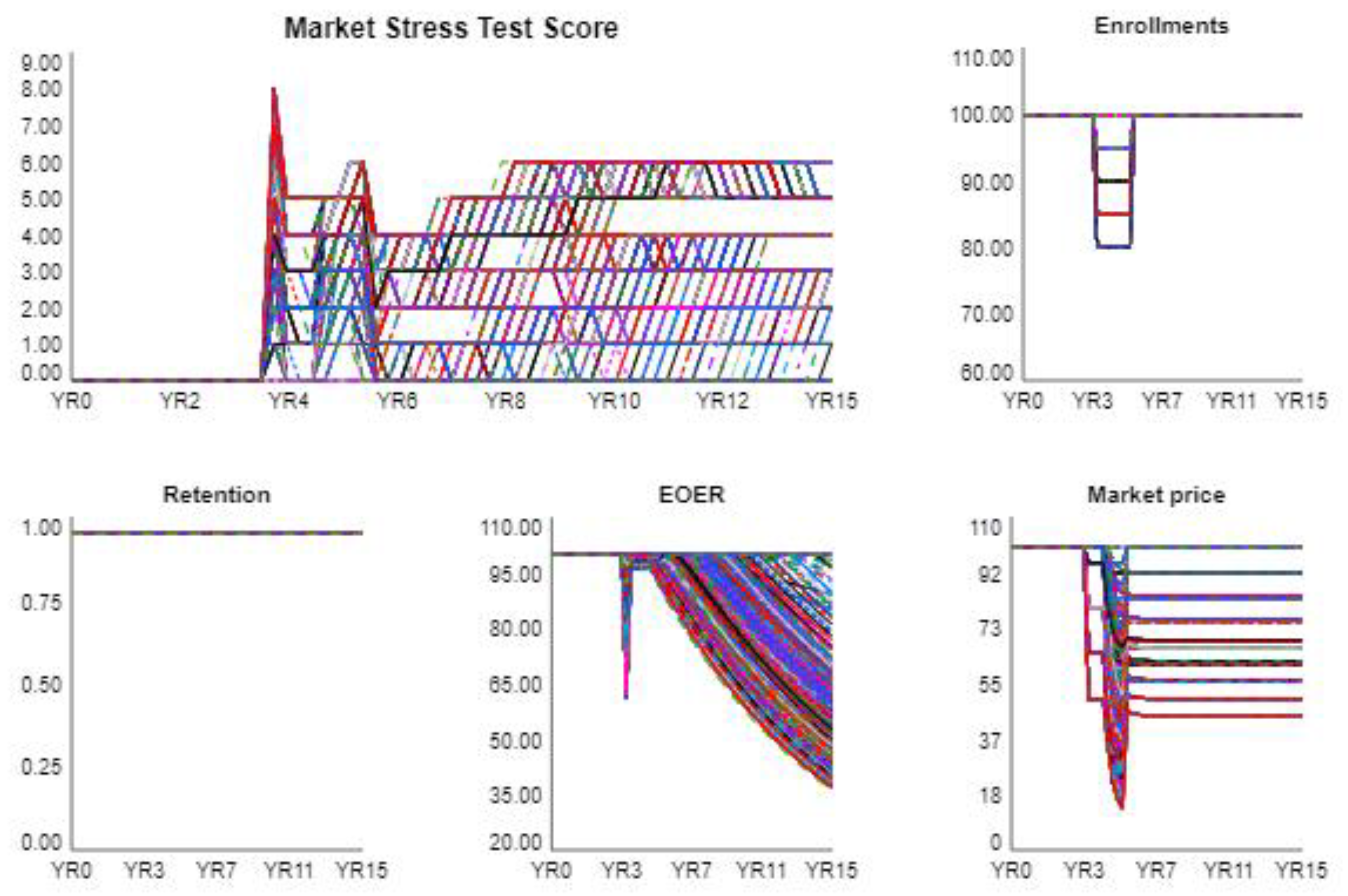
When all stressors are combined, the MSTS index rises as high as 8 during the pandemic and may stay as high as 6 beyond the pandemic for certain parameter value combinations (Figure 16). While this article does not examine changes in the student retention, the other three contributors to MSTS (enrollments, EOER, and the market price) cause the index to spike during the pandemic and keep it within the high range beyond the pandemic. While enrollments stabilize after the pandemic (see Figure 16), the drop in the market price and the low scores for the endowment-to-operating expenses ratio (EOER) contribute to the high MSTS scores, which indicate the long-term financial vulnerability of the college.

6. Discussion

The COVID-19 pandemic had a major impact on the global economy, and it disrupted most economic sectors including higher education. Extreme events such as a global pandemic provide opportunities to learn a great deal about the resilience of higher education institutions.

6.1. Research Contribution

Organizational responses to the COVID-19 pandemic are an active research area (e.g., [55]). A number of studies have examined the effect of the pandemic on higher education. For example, Aristovnik et al. [56] surveyed student perceptions and satisfaction during the COVID-19 crisis. Wildman et al. [3] and Losina et al. [28] studied the trade-offs between health outcomes and the cost of mitigation approaches. To the best of our knowledge, this article is the first scholarly study of the impact of COVID-19 on the financial sustainability of academic institutions.

This study adopts a systems view of a college, which has been identified as a powerful methodological lens for the analysis of complex problems [14,15,16,29], including in higher education [8,9,10,23,30,31,32,33]. Because colleges are highly interconnected and non-linear systems, any academic scenario planning must involve computational experiments to account for the important forces that influence organizational performance [9,22,23,24,25]. Moreover, higher education resource planning and management requires balancing competing interests of multiple stakeholders [9,11,21], which necessitates a systems approach to the planning process.

By developing a dynamic theory of academic institutions and the forces that determine their survival or failure in the face of the COVID-19 pandemic, this article adds to the literature on the management of the pandemic-related risk, college stress-testing and model-informed decision making in higher education. The article extends the theory developed in the college model [6], which studied the effects of demographic changes in higher education. We start with identifying the effects of the pandemic, then we map those effects in a causal loop diagram, and finally we build a rigorous computational model and perform simulation experiments that characterize the financial sustainability and resilience outcomes of academic institutions. Our analysis integrates the market stress test framework developed by Zemsky et al. [17]. We show that the COVID-19 shock can propagate widely through the college in the short and long term.

6.2. Implications for Practice

Our work provides several lessons for leaders of academic institutions. It shows that when institutions are confronted with a major shock, such as a pandemic, the leadership needs to take a “systems thinking” view of the situation. They need to think of the numerous effects of the shock (pandemic) and understand how those effects impact the entire organization and the financial sustainability outcomes over time. They need to map and define the important complex causal chains and feedback loops that drive system behavior over time, as shown in our framework (Figure 2). Due to complex causality, delays and feedback loops, the behavior of an organization is often counterintuitive and difficult to comprehend. Failure to take a systems approach that recognizes complex causality, delays and respects feedback thinking may lead to choices that have unintended consequences.

Our analysis shows that a healthy emergency cash reserve and a substantial endowment might be critical when an academic institution experiences an external shock, such as a COVID-19 pandemic. Simulations also suggest that consequences of the pandemic might be felt by colleges for a long time, and certain combinations of mitigation polices can be especially damaging for the long-term financial sustainability of academic institutions.

To recover from the pandemic, colleges may need to increase revenue and cut costs, even though, in a recent survey, 48 percent of Chief Business Officers indicated that their academic institutions cannot cut expenses without sacrificing quality [47]. A typical pre-pandemic approach to boosting revenue had been to increase tuition and enrollment and launch new programs [47]. However, moving forward, increasing tuition or enrollment might be challenging considering that it can take time for families to recover from the economic losses due to the pandemic and because the college-age population is on a decline. Launching new programs might be difficult too at the time when academic institutions must be vigilant about their expenditures.

We conclude that as colleges face multiple existential threats and challenges, they need to rethink the provision of educational and auxiliary services in order to improve the sustainability of their business models. One potential approach is to leverage business model innovation and new technologies such as artificial intelligence [57]. That should be an important direction for research on the future of higher education.

7. Conclusions

This article built a computational model to study the impact of COVID-19 on the financial sustainability of higher education institutions. Computational experiments added to our theoretical understanding of what makes an institution financially sustainable and resilient. It also provided insights for the higher education sector that has to navigate major crises such as the global pandemic.

The limitations of this article are model assumptions that could be relaxed in future research studies. For example, we assume that institutions are not limited in how much they can borrow. Additionally, students may continue to choose to live off campus for some time even if everything goes back to in-person, especially those students who can afford it. It may take longer for enrollments to return to the pre-pandemic levels given the higher financial need of students and the institutions’ need to maintain a certain tuition. Even after the pandemic is officially over, some COVID-19 testing may still be necessary, and colleges may still need to sanitize rooms and re-fit classrooms for continued social distancing.

The framework developed in this article can be turned into a system-dynamics based interactive learning environment, SDILE, which is a tool for improving decision making in dynamic tasks [58]. It can also be part of a personalized and adaptive online interactive learning environment, OILE, [59] used during an institutional planning process. By interacting with such learning environments, individuals can improve structural knowledge, decision heuristics, and decision time leading to better strategies [59,60]. To improve their efficacy, such decision support systems can be combined with prior exploration [61] and debriefing [62,63,64].

References

1. Diep, F. The 5 Biggest Lessons We’ve Learned about How Coronavirus Spreads on Campus. The Chronicle of Higher Education, 3 December 2020. [Google Scholar]
2. Bauman, D. A Brutal Tally: Higher Ed Lost 650,000 Jobs Last Year. The Chronicle of Higher Education. 5 February 2021. Available online: https://www.chronicle.com/article/a-brutal-tally-higher-ed-lost-650-000-jobs-last-year (accessed on 5 March 2021).
3. Wildman, W.J.; Diallo, S.Y.; Hodulik, G.; Page, A.; Tolk, A.; Gondal, N. The Artificial University: Decision Support for Universities in the COVID-19 Era. Complexity 2020, 2020, 1–10. [Google Scholar] [CrossRef]
4. Wescott, D. Will Coronavirus Close Your College for Good? The Chronicle of Higher Education. 25 March 2020. Available online: https://www.chronicle.com/article/will-coronavirus-close-your-college-for-good/ (accessed on 1 February 2021).
5. Council on Competitiveness. Elevate. Optimizing the Role of Higher Education in the Emerging Innovation Landscape; The Council on Competitiveness: Washington, DC, USA, 2019. [Google Scholar]
6. Pavlov, O.V.; Katsamakas, E. Will colleges survive the storm of declining enrollments? A computational model. PLoS ONE 2020, 15, e0236872. [Google Scholar] [CrossRef] [PubMed]
7. Lindner, A. Declining College Enrollments: A System Dynamics Approach. 2020. Available online: https://www.informs.org/Publications/OR-MS-Tomorrow/Declining-College-Enrollments-A-System-Dynamics-Approach (accessed on 2 February 2021).
8. Lella, G.A.; Fischetto, V.; Cesarotti, J.C.; Spohrer, G.; Leung, Y.T. Universities as complex service systems: External and Internal perspectives. In Proceedings of the IEEE International Conference on Service Operations and Logistics, and Informatics (SOLI), Suzhou, China, 8–10 July 2012. [Google Scholar]
9. Massy, W. Reengineering the University: How to Be Mission Centered, Market Smart, and Margin Conscious; Johns Hopkins University Press: Baltimore, MD, USA, 2016. [Google Scholar]
10. Rouse, W.B. Universities as Complex Enterprises: How Academia Works, Why It Works These Ways, and Where the University Enterprise Is Headed; Wiley: Hoboken, NJ, USA, 2016. [Google Scholar]
11. Kezar, A. How Colleges Change: Understanding, Learning, and Enacting Change; Routledge: New York, NY, USA, 2018. [Google Scholar]
12. Pavlov, O.; Hoy, F. Toward the Service Science of Education. In Handbook of Service Science; Springer: New York, NY, USA, 2019; Volume 2, pp. 545–566. [Google Scholar]
13. Vedder, R.K. Restoring the Promise: Higher Education in America; Independent Institute: Oakland, CA, USA, 2019. [Google Scholar]
14. Maani, K.E.; Cavana, R.Y. Systems Thinking, System Dynamics: Managing Change and Complexity; Pearson Education New Zealand: North Shore, New Zealand, 2007. [Google Scholar]
15. Morecroft, J. Strategic Modelling and Business Dynamics: A Feedback Systems Approach; John Wiley & Sons: Oxford, UK, 2007. [Google Scholar]
16. Duggan, J. System Dynamics Modeling with R; Springer: New York, NY, USA, 2016. [Google Scholar]
17. Zemsky, R.; Shaman, S.; Baldridge, S.C. The College Stress Test: Tracking Institutional Futures across a Crowded Market; Johns Hopkins University Press: Baltimore, MD, USA, 2020. [Google Scholar]
18. Natow, R.S. Why Haven’t More Colleges Closed? Prognosticators Predicted Mass Shutterings. That Hasn’t Happened, But Other Enormous Changes Are Underway. The Chronicle of Higher Education. 1 March 2021. Available online: https://www.chronicle.com/article/why-havent-more-colleges-closed (accessed on 5 March 2021).
19. Levine, J.B. Application of the CAMPUS simulation models to the major planning decisions of a large university. In Proceedings of the 2nd Conference on Applications of Simulations, New York, NY, USA, 2–4 December 1968; pp. 317–328. [Google Scholar]
20. RRC. The Development of a Computer Model for Projecting Statewide College Enrollments: A Preliminary Study; Rensselaer Research Corp.: Troy, NY, USA, 1968. [Google Scholar]
21. Townsley, M.K. The Small College Guide to Financial Health: Beating the Odds; NACUBO: Washington, DC, USA, 2002. [Google Scholar]
22. Galbraith, P.L. System Dynamics and University Management. Syst. Dyn. Rev. 1998, 14, 69–84. [Google Scholar] [CrossRef]
23. Kennedy, M.; Clare, C. Some issues in building system dynamics model for improving the resource management process in higher education. In Proceedings of the 17th International System Dynamics Conference, Wellington, New Zealand, 20–23 July 1999. [Google Scholar]
24. Rodríguez, J.C.; Gómez, M.; Serna, M. Complexity in Managing Higher Education Institutions in Mexico: A System Dynamics Approach. Int. J. Educ. Pedagog. Sci. 2016, 10, 3946–3953. [Google Scholar]
25. Massy, W.F. Resource Management for Colleges and Universities; Johns Hopkins University Press: Baltimore, MD, USA, 2020. [Google Scholar]
26. Mansmann, S.; Scholl, M.H. Decision Support System for Managing Educational Capacity Utilization. IEEE Trans. Educ. 2007, 50, 143–150. [Google Scholar] [CrossRef] [Green Version]
27. Webber, K.L.; Zheng, H.Y. Data Analytics and the Imperatives for Data-Informed Decision Making in Higher Education. In Big Data on Campus; Johns Hopkins University Press: Baltimore, MD, USA, 2020; pp. 3–29. [Google Scholar]
28. Losina, E.; Leifer, V.; Millham, L.; Panella, C.; Hyle, E.P.; Mohareb, A.M.; Neilan, A.M.; Ciaranello, A.L.; Kazemian, P.; Freedberg, K.A. College Campuses and COVID-19 Mitigation: Clinical and Economic Value. Ann. Intern. Med. 2020. [Google Scholar] [CrossRef]
29. Galbraith, P.L. System Dynamics: A Lens and Scalpel for Organizational Decision Making. OR Insight 2010, 23, 96–123. [Google Scholar] [CrossRef]
30. Frances, C.; Alstyne, M.V.; Ashton, A.; Hochstettler, T. Using System Dynamics Technology to Improve Planning and Budgeting for Higher Education: Results in Arizona and Houston, Texas. In Proceedings of the International System Dynamics Conference, Sterling, Scotland, 11–15 July 1994. [Google Scholar]
31. Bell, G.; Cooper, M.; Kennedy, M.; Warwick, J. The development of the Holon planning and costing framework for higher education management. In Proceedings of the 18th System Dynamics Conference, Bergen, Norway, 6–10 August 2000. [Google Scholar]
32. Barnabe, F. From Ivory Towers to Learning Organizations; the Role of System Dynamics in the Managerialization of Ac-ademic Institutions. In Proceedings of the 22nd System Dynamics International Conference, Oxford, UK, 25–29 July 2004. [Google Scholar]
33. Oyo, B.; Williams, D. Re-conceptualisation of higher education quality management problems using feedback systems thinking. Int. J. Manag. Educ. 2009, 3, 220. [Google Scholar] [CrossRef]
34. Forrester, J.W. Industrial Dynamics; Productivity Press: Cambridge, MA, USA, 1961. [Google Scholar]
35. Georgantzas, N.C.; Katsamakas, E.G. Information systems research with system dynamics. Syst. Dyn. Rev. 2008, 24, 247–264. [Google Scholar] [CrossRef]
36. Georgantzas, N.C.; Katsamakas, E.G. Performance effects of information systems integration: A system dynamics study in a media firm. Bus. Process Manag. J. 2010, 16, 822–846. [Google Scholar] [CrossRef]
37. Miesing, P.; Krzykowski, L.; Rich, E. Enabling sustainability in management education. In Handbook of Sustainability in Management Education; Edward Elgar Publishing: Cheltenham, UK, 2017; pp. 539–566. [Google Scholar]
38. Saysel, A.K. Role of Information Feedback in Soil Nitrogen Management: Results from a Dynamic Simulation Game. Syst. Res. Behav. Sci. 2017, 34, 424–439. [Google Scholar] [CrossRef]
39. Jahangirian, M.; Eldabi, T.; Naseer, A.; Stergioulas, L.K.; Young, T. Simulation in manufacturing and business: A review. Eur. J. Oper. Res. 2010, 203, 1–13. [Google Scholar] [CrossRef] [Green Version]
40. Davidsen, P.I.; Kopainsky, B.; Moxnes, E.; Pedercini, M.; Wheat, I.D. Systems Education at Bergen. Systems 2014, 2, 159–167. [Google Scholar] [CrossRef] [Green Version]
41. Pavlov, O.V.; Doyle, J.K.; Saeed, K.; Lyneis, J.M.; Radzicki, M.J. The Design of Educational Programs in System Dynamics at Worcester Polytechnic Institute (WPI). Systems 2014, 2, 54–76. [Google Scholar] [CrossRef]
42. Schaffernicht, M.F.G.; Groesser, S.N. A Competence Development Framework for Learning and Teaching System Dynamics. Syst. Dyn. Rev. 2016, 32, 52–81. [Google Scholar] [CrossRef] [Green Version]
43. Cavana, R.Y.; Forgie, V.E. Overview and Insights from Systems Education for a Sustainable Planet. Systems 2018, 6, 5. [Google Scholar] [CrossRef] [Green Version]
44. Zaini, R.M.; Pavlov, O.; Saeed, K.; Radzicki, M.; Hoffman, A.; Tichenor, K. Let’s Talk Change in a University: A Simple Model for Addressing a Complex Agenda. Syst. Res. Behav. Sci. 2017, 34, 250–266. [Google Scholar] [CrossRef]
45. Howard, C.; Higher-Education Bonds in a COVID-19 World. Charles Schwab Bond Insights. 22 June 2020. Available online: https://www.schwab.com/resource-center/insights/content/higher-education-bonds-COVID-19-world (accessed on 3 November 2020).
46. NACUBO. NACUBO-TIAA Study of Endowments; NACUBO: Washington, DC, USA, 2020. [Google Scholar]
47. Lederman, D.; Jaschik, S. The 2018 Inside Higher Ed Survey of College and University Business Officers; Inside Higher Ed and Gallup: Washington, DC, USA, 2018. [Google Scholar]
48. Sedlacek, V. The Importance of Stress Testing in Higher Education. Available online: https://agb.org/trusteeship-article/the-importance-of-stress-testing-in-higher-education/ (accessed on 5 March 2021).
49. Saeed, K. Slicing a complex problem for system dynamics modeling. Syst. Dyn. Rev. 1992, 8, 251–261. [Google Scholar] [CrossRef]
50. ACHA. The COVID-19 Pandemic’s Effect on Campus Health and Well-Being Services: A Snapshot of Operating Status and Response; American College Health Association: Silver Spring, MD, USA, 2020. [Google Scholar]
51. National Student Clearinghouse. Current Term Enrollment Estimates. 17 December 2020. Available online: https://nscresearchcenter.org/current-term-enrollment-estimates/ (accessed on 18 December 2020).
52. Korn, M. Ivy League Colleges Report Dramatic Growth In Early-Admission Applicant Pools. Wall Street J. 2020. Available online: https://www.wsj.com/articles/ivy-league-colleges-report-dramatic-growth-in-early-admission-applicant-pools-11608308681 (accessed on 15 December 2020).
53. Korn, M. Fewer High School Seniors Seek College Financial Aid, Raising Concerns About Their Plans. Wall Street J. 2020. Available online: https://www.wsj.com/articles/fewer-high-school-seniors-seek-college-financial-aid-raising-concerns-about-their-plans-11607176800 (accessed on 3 December 2020).
54. Zalaznick, M. 6 Demands Students Are Making in Columbia Tuition Strike. 2020. Available online: https://universitybusiness.com/students-demand-columbia-university-tuition-strike-financial-aid/ (accessed on 2 December 2020).
55. Dwivedi, Y.K.; Hughes, D.L.; Coombs, C.; Constantiou, I.; Duan, Y.; Edwards, J.S.; Gupta, B.; Lal, B.; Misra, S.; Prashant, P.; et al. Impact of COVID-19 pandemic on information management research and practice: Transforming education, work and life. Int. J. Inf. Manag. 2020, 55, 102211. [Google Scholar] [CrossRef]
56. Aristovnik, A.; Keržič, D.; Ravšelj, D.; Tomaževič, N.; Umek, L. Impacts of the COVID-19 Pandemic on Life of Higher Education Students: A Global Perspective. Sustainability 2020, 12, 8438. [Google Scholar] [CrossRef]
57. Katsamakas, E.; Pavlov, O.V. AI and Business Model Innovation: Leveraging the AI Feedback Loop. SSRN Electron. J. 2019, 8, 22–30. [Google Scholar] [CrossRef]
58. Qudrat-Ullah, H. Improving Human Performance in Dynamic Tasks: Applications in Management and Industry; Springer: New York, NY, USA, 2019. [Google Scholar]
59. Tadesse, A.T.; Davidsen, P.I. Framework to support personalized learning in complex systems. J. Appl. Res. High. Educ. 2019, 12, 57–85. [Google Scholar] [CrossRef]
60. Kopainsky, B.; Sawicka, A. Simulator-supported descriptions of complex dynamic problems: Experimental results on task performance and system understanding. Syst. Dyn. Rev. 2010, 27, 142–172. [Google Scholar] [CrossRef]
61. Kopainsky, B.; Alessi, S.M.; Pedercini, M.; Davidsen, P.I. Effect of Prior Exploration as an Instructional Strategy for System Dynamics. Simul. Gaming 2015, 46, 293–321. [Google Scholar] [CrossRef] [Green Version]
62. Qudrat-Ullah, H. Debriefing can reduce misperceptions of feedback: The case of renewable resource management. Simul. Gaming 2007, 38, 382–397. [Google Scholar] [CrossRef]
63. Grund, C.K.; Schelkle, M. Developing Serious Games with Integrated Debriefing. Bus. Inf. Syst. Eng. 2019, 62, 87–101. [Google Scholar] [CrossRef]
64. Pavlov, O.V.; Saeed, K.; Robinson, L.W. Improving Instructional Simulation with Structural Debriefing. Simul. Gaming 2015, 46, 383–403. [Google Scholar] [CrossRef]
Figure 1. The four modules of the college model.
Sustainability 13 03903 g001
Figure 2. Six components of the COVID-19 shock that are studied in this article and their impact on a college.
Sustainability 13 03903 g002
Figure 3. The dynamics of fewer students on campus (S1). The base case is when 100 percent of students remain on campus. We simulate four scenarios when 90, 60, 30, and 0 percent of student stay on campus.
Sustainability 13 03903 g003
Figure 4. Sensitivity runs for the market stress test score (MSTS) and its components when fewer students are on campus. The runs are scenarios when 100, 90, 60, 30, and 0 percent of students remain on campus.
Sustainability 13 03903 g004
Figure 5. The dynamics of enrollment decline (S2). We simulate a case when only a fraction of a typical incoming class of students enroll during the pandemic. The base case is compared to the scenarios when 95, 90, 85, and 80 percent of a regular class enroll.
Sustainability 13 03903 g005
Figure 6. The market stress test score and its components when enrollment declines (S2). The base case is compared to the scenarios when 95, 90, 85, and 80 percent of a regular class enroll.
Sustainability 13 03903 g006
Figure 7. The effect of COVID-19 preparedness (S3). These scenarios simulate a one-time expense by the college on COVID-19 preparedness measures. We assume that the cost of COVID-19 preparedness can be 4, 8, 16, or 32 $/sq ft, which is compared to the base case when the cost is 0 $/sq ft.
Sustainability 13 03903 g007
Figure 8. Sensitivity runs for the market stress test score and its components to account for COVID-19 preparedness (S3). We assume that the cost of COVID-19 preparedness can be 4, 8, 16, or 32 $/sq ft, which is compared to the base case when the cost is 0 $/sq ft.
Sustainability 13 03903 g008
Figure 9. Effects due to expenses associated with the health and safety measures (S4). We assume that all students are tested 16, 32, or 64 times a year. In the steady state, students are not tested (0 tests).
Sustainability 13 03903 g009
Figure 10. The market stress test score and its components for health and safety runs (S4). We assume that all students are tested 16, 32, or 64 times a year. In the steady state, students are not tested (0 tests).
Sustainability 13 03903 g010
Figure 11. The dynamics when more financial aid is allocated (S5). The simulations assume that the pre-pandemic steady state tuition discount rate is 40 percent. When financial aid increases, the tuition discount rates become 45, 50, 55, and 60 percent.
Sustainability 13 03903 g011
Figure 12. The market stress test score and its components when more financial aid is allocated (S5). The simulations assume that the pre-pandemic steady state tuition discount rate is 40 percent. When financial aid increases, the tuition discount rates become 45, 50, 55, and 60 percent.
Sustainability 13 03903 g012
Figure 13. The dynamics of lower tuition (S6). These experiments assume that the tuition is reduced to $25,000, $20,000, $15,000, $10,000, while the steady state tuition prior to the pandemic is $30,000.
Sustainability 13 03903 g013
Figure 14. The market stress test score and its components when tuition is reduced (S6). These experiments assume that the tuition is reduced to $25,000, $20,000, $15,000, $10,000, while the steady state tuition prior to the pandemic is $30,000.
Sustainability 13 03903 g014
Figure 15. Trajectories of key variables during the combined sensitivity runs. We conduct 1000 runs for different combinations of parameter values from within the ranges specified for simulations S1–S6. The parameter values are picked using the Latin Hypercube sampling method.
Sustainability 13 03903 g015
Figure 16. The market stress test score and its components during the simulation of the combined effect of COVID-19 on an academic institution. We conduct 1000 runs for different combinations of parameter values from within the ranges specified for simulations S1–S6. The parameter values are picked using the Latin Hypercube sampling method.
Sustainability 13 03903 g016