Abstract
The latest studies have compellingly argued that Neural Networks (NN) classification and prediction are the right direction for forecasting. It has been proven that NN are suitable models for any continuous function. Moreover, these methods are superior to conventional methods, such a Box–Jenkins, AR, MA, ARMA, or ARIMA. The latter assume a linear relationship between inputs and outputs. This assumption is not valid for skimmed milk powder (SMP) forecasting, because of nonlinearities, which are supposed to be approximated. The traditional prediction methods need complete date. The non-AI-based techniques regularly handle univariate-like data only. This assumption is not sufficient, because many external factors might influence the time series. It should be noted that any Artificial Neural Network (ANN) approach can be strongly affected by the relevancy and “clarity” of its input training data. In the proposed Convolutional Neural Networks based methodology assumes price series data to be sparse and noisy. The presented procedure utilizes Compressed Sensing (CS) methodology, which assumes noisy trends are incomplete signals for them to be reconstructed using CS reconstruction algorithms. Denoised trends are more relevant in terms of NN-based forecasting models’ prediction performance. Empirical results reveal robustness of the proposed technique.
1. Introduction
International SMP prices have often been impacted by the significant influence of market volatility, seriously affecting the global economies, as well as the food market, food processors, and society in general.
First, similar to valuation of other commodities, SMP prices are fundamentally controlled by demand and supply. SMP, which is 34–35% protein, is the most common dairy ingredient used for numerous therapeutic and grocery products and supplementary foods. Moreover, SMP price is also intensely affected by other factors, such as cattle and bovine diseases (which can affect the demand curve), weather, natural disasters, drought, inventory, economic growth, financial and political policies (imply conditions in international business environment), regionally differentiated subsidies (common agricultural policy), changes in the international agro-food systems, and psychological expectations. These aspects relate to a heavily fluctuating SMP prices, characterized by strong complex nonlinearity, dynamic variation, and high volatility. In return, the SMP market irregularity has a major impact on the economy and societies; this influence on economies needs to be recognized to lower investment decision risk for agents and planners inside and outside the food supply chain.
One of the largest and more-dynamic financial markets is the SMP market, being among the most used and most important economic indices. Forecasting SMP rates is a problematic issue in either theoretical or practical science, because the SMP rates are affected by many factors (as highlighted above). Undoubtedly, there is a need for efficient statistical and econometric models. This problem has been widely recognized by researchers as a leading purpose of forecasting SMP rates. Despite many efforts, this problem remains one of the key challenges in the field of forecasting.
Skimmed milk powder can impact spending on food. Its expected impacts on the general food industry are important to policy makers and food chain planners globally [1]. The fluctuating prices of SMP can increase the risk of investing in stocks and financial safety, as well as impact the market players who suffer from the economic downturn because of the failure of manufacturing the contracted volumes of SMP-based food products [2].
As shown in [3], the week-ahead dairy product spot price is affected by many uncorrelated factors, including week-ahead forecasts. The relationships between several external factors and spot prices have been proved not only to exist but also to be time dependent and nonlinearity associated.
The impact of SMP prices on the market, outlined in the above-mentioned studies, prompts a study of the problematic nature of predicting the SMP price time series. This need also reveals a gap in available tools for accurately forecasting SMP prices. If a more accurate tool were developed, then the undesirable influences of dairy substrates could be mitigated and could keep dairy prices stable.
The authors of [4,5] showed the versatility of numerous available prediction algorithms and the requirement for comparisons to examine which methodologies perform better, in which circumstances and why. It should be noted that this study made on SMP forecasting methods revealed a serious research gap. However, time-series forecasting has received extensive attention in the research community.
Numerous reviews of several methods, models, and approaches for dairy product price forecasting can be found in [6,7,8,9,10].
Time-series-based values estimation is a difficulty for many engineering sciences. Traditional prediction approaches make use of direct future value calculation, based on its past linear combination. There are comprehensive studies [11,12,13,14,15,16,17] in this area that reveal numerous applications in fields such as economics, econometrics, finance, and stock forecasting.
The authors of [18] made significant work in considering the applications made of numerical linear models. These models utilize Autoregressive (AR) and Moving Averages (MA) concepts. The AR procedure necessitates the expectation that the current estimation of the time arrangement is a linear combination of its past predecessors. Procedures in MA assume that the current value can be represented by a combination of random passes or noise, which influence the time series. These kinds of approaches have proved their usability in the field of the dynamics of many real-time series.
Nevertheless, because of assumed linearities, these models are insufficient in mimicking the nonlinear nature of real dynamics, which can occur in practical applications [19,20]. Therefore, it should be noted that numerous authors have proposed adaptable numerical models based on AI. The use of NN allows for more accurate forecasting because they can consider using nonlinearities in raw material [21,22,23]. Another approach is concentrated on the use of single-multi-step forecasting procedures [22,24].
The main contributions of this paper are summarized as follows: (1) A deep learning-based prediction algorithm has never been applied to agricultural economics before. However, it seems that CNNs have never been used thus far to perform skimmed milk powder forecasting. Additionally, the presented combination of the compressed-sensing based training sets denoising and convolutional neural networks has never been presented by any author thus far in the literature. The proposed algorithm outperforms all the state-of-the-art competitors. The remainder of this paper is organized as follows. Section 2 discusses how artificial intelligence struggles with forecasting issues. Section 3 and Section 4 emphasize the compressed sensing-convolutional neural networks, i.e. the proposed forecasting procedure, and the methods and materials, respectively. Finally, Section 5 focuses on the achieved results and discusses them. The final section discusses the conclusions and future research directions.
2. Artificial Intelligence Struggles with Forecasting Issues
Artificial Neural Networks (ANN)-based forecasting methods have received special attention in the recent years due in part to their flexibility and capability of future value modeling. The most recent methods exploit ANN topologies while including a nonlinearity-based AR model, as well as a dynamic architecture component at its core [25]. Some other papers make use of the AR neural networks [26,27,28] and force the AR model to include nonlinear functions. Moreover, the authors proposed the use of multilayer-perceptron linear model hybrid techniques [20].
Notwithstanding the accomplishment of ANN and its actual impact on science, it is evident that numerous issues remain open [29]. Several factors in practical modeling methods should be underlined. These factors are supposed to be considered abstractive and related to the past behavior of the process being modeled. In this way, these kinds of aspects are problematic in terms of including them in decision-making algorithm architectures [27].
Another serious obstacle that ANNs face is their exclusion of the MA models. Most of the proposed methods utilize a nonlinear AR model. Unfortunately, in those works, the MA model is not considered. This shortcoming leads to a misprediction [11]. For these reasons, AR and MA components need to be included. This inclusion allows AI-based prediction models to model both terms using their flexible frameworks [22].
Conventional stochastic and econometric models applied in financial time-series forecasting cannot efficiently handle the uncertain behavior of foreign exchange date series. The latest studies have revealed the classification and prediction efficiency of ANN. It has been proved that ANN can approximate any continuous function. The use of NNs in financial data-series forecasting has been compelling. These kinds of time-series prediction algorithms reveal their superiority over conventional methods such as Box–Jenkins, AR, ARMA, or ARIMA. Several impressive non-iterative approaches for solving the stated task were proposed by Roman Tkachenko and Ivan Izonin et al. [30,31,32].
The AI-based methods do not have to be triggered by any kind of a prior information on the data series. The authors used data series with weekly SMP prices starting from 2010 to 2017 provided by the Global Dairy Trade.
A feedforward network and a recurrent network [25] were implemented and compared. The feedforward network was taught by the standard backpropagation algorithm, while the recurrent one was triggered using a multi-stream method based on the Extended Kalman Filter [33].
Previous forecasting models were used as inspiration to overcome the obstacle of expressing highly nonlinear, hidden pattern of SMP stock prices.
In contrast to the methods such as ARIMA, AI-based algorithms are fully self-adaptable, nonlinearity tolerant, and data triggered. Moreover, stochastic data assumptions (e.g., linearity, regularity, and stationarity) are not needed by AI, whereas conventional methods require these assumptions. Accordingly, numerous AI procedures (e.g., NNs, genetic algorithms, and support vector machines) have been popularized in the forecasting field [34,35,36].
It should be noted that sone of the most serious obstacles for forecasting algorithms are their interactive complexity, dynamic nature, and constantly changing factors. These aspects produce high levels of noise, which influence the input data and, consequently, lead to a weak performance for the prediction algorithms. For these reasons, noise filtering can lead to improved efficiencies. Several denoising methods were proposed by numerous authors. Sang et al. [37] suggested a novel, entropy-related wavelet transform denoising algorithms for time series classification. In turn, He [38] presented a Slantlet denoising-associated least squares support vector regression (LSSVR) scheme for forecasting exchange rate. Faria [39] presented an exponential smoothing denoising-related NN model for predicting stock markets. Yuan [40] suggested a promising scheme by fusing the Markov-switching idea and the Hodrick–Prescott filtering for forecasting exchange rates. Nasseri [33] presented a fusion method employing the extended Kalman filter and genetic algorithm for predicting water demand. In turn, Bo-Tsuen Chen, et al. [41] transferred the Fourier transform framework into a fuzzy time series prediction scheme for stock prices. Sang [42] suggested a modified wavelet transform-based denoising framework.
The proposed algorithm is based on CS theory. The suggested preliminary data filtering exploits data sparsity. The CS framework-based denoising turns this weakness into a strength. CS algorithms have been used in data-collecting algorithms. This concept assumes that data in some orthogonal basis are redundant. In the suggested ANN-learning paradigm, the Compressed-Sensing-Denoising (CSD) is initially run. This running is considered a preliminary operation performed directly on SMP price time series data. The rationale behind this is to reduce the level of noise and to enhance prediction performance.
One caveat of forecasting procedures is that none can be perfect in every practical condition. Thus, more in-depth comparative studies and method evaluation should be carried out. The drawback of the existing propositions in stock price prediction literature is their (the propositions’) inability to accurately predict highly dynamic and fast-changing patterns in stock price movement. The current work attempts to address this shortcoming by exploiting the power of convolutional neural networks (CNN) in learning the past behavior of stock price movements and making a highly accurate forecast for future stock behavior [43].
In comparison to regular training paradigms, deep learning procedures, when combined with CSD denoising, are better in terms of their ability to generalize. The emphasis is on long short-term memory networks (LSTM) [27], ANN, attention-based models, and deep convolution networks (DCN) [44]. The SMP time series prediction is implemented by utilizing one deep-learning modeling structure, the so-called “Multiple Input, Multiple Output” (MIMO) method. This term refers to the initialization based on multiple input datasets (SMP prices). In this way, these method utilizes multiple sets of predictions as output (SMP and butter predictions).
The performance rates were calculated using established evaluation criteria (average gap, MSE, RMSE, and RMSLE) for every single procedure to assess the performance of the suggested and competitive solutions. The author’s contribution is to present a new approach to denoise the datasets for the deep learning paradigm by exploiting CS-based denoising procedures [45,46]. This method facilitates the assumption of training data to be sparse and incomplete. The CSD framework is suitable to reconstruct signals from their sparse representation. The application will deliver a smoother input training dataset for prediction models and, therefore, make the performance of the forecasting algorithm better. Furthermore, there is a chance in reducing mispredictions. The empirical results indicate that the LSTM topology has a strong nonlinear handling capability and is useful for computing non-stationary SMP forecasts.
3. Compressed Sensing-Convolutional Neural Networks: The Proposed Forecasting Procedure
Machine learning is a promising technique to overcome financial sector inconveniences. It has been argued that deep-learning techniques, including CNNs, have proved their worth in identifying, classifying, and predicting patterns and time series. It should be noted that CNN methods can handle inherent data complexities, e.g., spatio-temporality, chaotic nature, and non-stationarity, only in cases when they are designed and/or evaluated for each specific dataset and application. To let CNNs work, they need to be initialized with a large number of labels [47].
The deep learning methodology is based on machine learning paradigms and usually consists of two main stages: recurrent and convolutional neural networks. Typically, a CNN requires two-dimensional input images as its input vector. This requirement makes using CNNs in financial market prediction quite difficult. To solve this shortcoming, 1D matrices are supposed to be converted into 2D matrices [48].
In this work, a deep-learning-based, initially trained by compressively sensed datasets, SMP price movement forecasting algorithm is presented. Additionally, TensorFlow is applied to design the prediction model. The pipeline of the algorithm is organized as follows: the input data are preprocessed and normalized; this strongly implies further algorithm stages; and the next step is 1D convolution and indicating key features (e.g., volume, high and low price, and closing price) as input.
The Convolutional Neural Net is an example of feedforward neural net. Numerous similarities between typical NN typology and CNN can be noticed. It also consists of input, hidden, and output layers. The CNN extends its predecessor with convolution or pooling layers. Moreover, the number of hidden layers in a CNN is usually higher than in a typical NN, leading to extending the capability of the NN. The higher is the number of hidden layers, the higher is the ability of input extraction and recognition. The convolutional nets have found their applications in the fields of image processing, computer vision, human feature recognition, and image classification. Deep learning methodology has proven how efficient and superior it can be in numerous areas, such as pattern, speech, and voice recognition, decision making support systems, etc. [49,50,51,52,53,54]. The neural net models with extended topologies, such as CNNs and RNNs, have significantly improved performance.
The data of the SMP prices and Google trends data are used as the input to a RNN, which is taught to forecast the complexity of the SMP market. The training method proposed in this paper is based on the following stages: the training dataset is first compressively sensed to denoise it. After that, a denoised large-scale dataset with more than four-million limit orders is applied to train the CNNs for stock price movements. This training paradigm is combined with a normalization process which considers the fluctuations in the price ranges among different stocks and time periods; this combination turned out to be a crucial factor for effectively scaling to big data.
Every financial market is associated with a limit order, which is a kind of order to buy or sell some number of shares at a set price [55]. Therefore, the order book has two points of view: the one associated with the bid prices with corresponding volume and the other associated with sell prices with corresponding volume . Both sets are sorted by price, where represents the highest offered buy price and refers to the lowest offered sell price. When a bid order price is higher than an ask order price, , they are removed, triggering the execution of the orders and exchanging the traded assets between the people involved in the market. When the orders are not the same in terms of their volume sizes, the bigger one remains in the order book while keeping the volume unfulfilled.
Numerous tasks are associated with these data, i.e., price trend forecasting and the regression of the predicted value of a metric, e.g., capability to o the detection of unexpected events that lead to price jumps as well as volatility of a stock. However, recognizing these aspects is obviously helpful in making the right investment decisions. The procedures frequently undersample the data, using specialized procedures such as Open-High-Low-Close (OHLC) [56] to maintain a representative number of samples for an assumed period. OHLC does not preserve all the microstructure information of the markets.
CNNs can be used to fix the problem since they can exploit all the information nested in the data, due in part to their ability to more precisely select and use recurring patterns between time steps. Assuming that the input datasets are denoised, they can actually feed into long short-term memory networks (LSTM) schemes to exploit sets of price time series with a determined width as input and, therefore, create a new series of encoding. Meanwhile, the just generated sequence of encoding will trigger the attention mechanism to improve its temporal attributes.
The next stage of the algorithm involves processing by the Convolution Neural Network (CNN) core, which delivers spatial features from the output dataset. The number of variables or redundant attributes are reduced by the Max Pooling layer (see Figure 1).
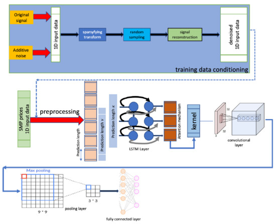
Figure 1.
The presented algorithm’s flowchart.
At the last stage of the procedure, the fully-connected layer with the linear activation function produces the network’s output, which is an equivalent of the prediction of tendency for SMP price.
3.1. Initial Denoising: The Training Data Conditioning
Compressed sensing is well known as a signal processing technique for efficiently acquiring and reconstructing a signal, by finding solutions to underdetermined linear systems. The compressed sensing (CS) reconstruction algorithm intends to recover a structured signal acquired using a small number of randomized measurements. Time series image denoising can be considered to be recovering a signal from inaccurately and/or partially measured samples, which is exactly what compressive sensing accomplishes.
Because of the complexity of noise nature, noise removal procedures are supposed to be well recognized and addressed by specialized techniques. In this paper, a novel improved compressed sensing based denoising method is presented, as shown in Figure 2 and Table 1. The proposed denoising algorithm assumes that training sets are noisy and in this way incomplete. Typical CS reconstruction algorithms can be cast as iteratively estimating a signal from a distorted observation. This process refers to training sets denoising.
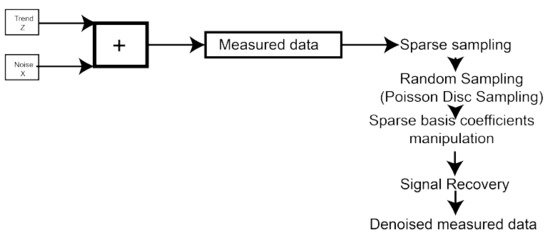
Figure 2.
The presented compressed-sensing based training datasets denoising algorithm’s flowchart.

Table 1.
Compressed Sensing based denoising of original data.
The well-recognized, fundamental signal processing theorem—Shannon’s sampling theorem—states that perfect signal reconstruction is doable if frequency sampling is at least two times greater than the maximum frequency of the signal. The compressed sensing methodology has none of these kinds of limitations in performing perfect signal reconstruction because signal sparsity can be exploited. In practice, some other conditions under which recovery is possible must also be satisfied. The above-mentioned signal sparsity requires the signal to be sparse in some domain. Moreover, signal incoherence, which is applied through the isometric property, is considered to meet the requirements for sparse signals.
An underdetermined set of linear equations has more unknowns than equations and generally has an infinite number of solutions. In this way, there is an equation system where we want to find a solution for x. To calculate a solution to this kind of system, one must enforce more constraints or conditions (e.g., smoothness). In the case of the compressed sensing, the constraint of sparsity is added, accepting only the solutions with a minimum number of nonzero coefficients. Not every kind of underdetermined system of linear equations can have a sparse solution. Hopefully, the compressed sensing methodology, with its support for sparse sampling, allows the recovery of that solution.
Compressed sensing methodology takes advantage of various kinds of redundancies in proper domains. This assumption allows a reduction of the number of coefficients, which leads to measurements acquisition acceleration.
Initially, the L2 norm was suggested as the main operation performed to minimize the energy in the system. This procedure, being quite simple from a computational point of view, usually provides poor results for the majority of practical cases, for which the unknown coefficients have nonzero energy.
Any historical stock data price can contain a finite amount of noise. The so-called “basis pursuit” denoising has been frequently suggested [57] over linear programming. This denoising technique preserves the signal sparsity in the presence of noise and can be solved quicker than an exact linear program.
For time series denoising, we first transform the noisy time series into the sparse domain using:
where z denotes the additive noise. is being sparsely sampled by mixing matrix where M is stable and incoherent with the matrix transform:
and , which would be called the compressed sensing matrix A.
According to the noisy time series , we want to restore the original time series from the noisy one. It has been proved that sparsity is a basic principle in signal restoration.
Besides, it is obvious that the noise is not sparse in the relevant orthogonal transform domain. In this way, the exact signal can be reconstructed from its sparsely sampled representation.
The compressed sensing-based denoising procedure is performed in the following way:
A CS reconstruction procedure attempts to reconstruct a signal obtained using a minimum number of randomized readouts. Regular CS restoration procedures can be interpreted as calculating a signal from a noisy observation in an iterative manner. In this algorithm, an unknown noisy time series is observed (sensed) through a limited number linear functional in random projection, and then the original time series is reconstructed using the observation vector and the existing reconstruction procedures such as L1 minimization [58].
Behind the applications such medical modalities or telecommunications, CS can be applied in the field of big data denoising. Preliminary attempts to exploit this methodology in the field of data were suggested by [59,60].
Formally, in a relevant basis, sparse signals can be interpreted in the following way. Technically, a vector is expressed in a convenient orthonormal basis in the following way:
where denotes ith coefficient set of X and .
In this way, X is composed of , where is an matrix with as columns. The sparsity of X can be directly controlled by the zero entries.
To perform the compressed based denoising, the following steps are needed:
- Sparse representation.Assuming that the is sparse in an orthogonal basis , the sparse coefficients B can be expressed as .
- Random sampling.The dimensional observation matrix is defined in the following way. More precisely, an observation vector Y is expressed using the random sampling matrix and sparse signal representation defined in the way below.In this paper, the random sampling is performed accordingly to the Poisson–Disk Sampling scheme, see Figure 3.
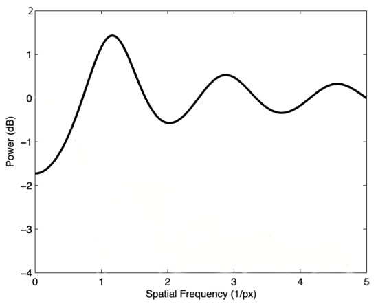 Figure 3. The average power spectrum of a 1D Poisson-disc process is related to a blue noise spectrum.
 - Signal recovery.The main goal of the signal recovery stage is to recover the signal X from the compressively sensed signal Y. This operation is expressed as follows:The equation above is not suitable for polynomial-time non-deterministic hard problems. For this reason, L0 norm is supposed to be replaced with L1 norm in the following way:Assuming that the signal X is affected by noise, the minimization problem needs to be reformulated in the following way:This optimization problem can be fixed by the orthogonal matching pursuit (OMP) algorithm. The signal X is compressively sensed in its relevant orthogonal domain, see Table 1. The SMP price time series is illustrated in Figure 3.The CS-based denoising algorithms assume that the native time series samples consist of trend values + noise. The principal goal of the method is to eliminate the noise. The denoising process shrinks the dimensions of the original time series.Traditionally, for instance, Fourier basis-based filtering is much tighter in terms of its initial parameters such as pass/stop frequencies. The CS-based noise removing is more adaptable because its only need is to choose proper orthogonal basis and frequency sampling.
3.2. Data Preprocessing
A preliminary analysis was conducted on SMP prices. The dataset published by the Global Dairy Trade contains SMP transaction records from 2000 to 2020. To make the CNN-based forecasting model workable, initial data standardization is needed. In this paper, the Standard Scale is exploited. In this regard, standard scalar calculations are performed in the way expressed below:
where denotes the value in the SMP time series data over some period (e.g., every two weeks).
An input datum is supposed to be windowed with a specified width, which is denoted as . In this paper, , which is related to two trading days per month.
In this way, a vector is converted into .
3.3. LSTM Component
Long short-term memory networks (LSTM) are artificial recurrent neural networks, which were initially presented by Hochreiter and Schmidhuber [27] and extended by Graves [50].
In the neural nets’ topology presented in this paper, the LSTM component consists of three layers: input layer, LSTM unit layer, and an output layer, with their own end-to-end feature.
The scheme operates using as the number of layers of LSTM, which is its controllable parameter.
For a given time sequence T, the input vector is fed into LSTM units to achieve comprehensive information from the previous steps and the future ones by the LSTM component.
The LSTM component consists of three gates: input, output, and forget gates. The input gate controls the extent to which a new value steps into the unit. The forget gate decides which values need to be kept or rejected. The output gate in turn determines the value of the LSTM unit’s output.
These operations can be expressed as follows:
where denotes the input vector. The flows into the LSTM unit, while is its output vector. , and are the weighted matrices and bias vector parameters, respectively. Moreover, the initial values are denoted as and . The operator ∘ refers to the element-wise product. and are sigmoid function and hyperbolic tangent functions. The product of the LSTM component is being sent to the attention mechanism.
3.4. Attention Mechanism
The resulting sequence of the LSTM unit feds into the attention mechanism (AM). Because of the high dimensionality of the input time series, the result is highly dependent on the number of LSTM processing units which are declined. To more efficiently uptake the relevant information from the new encoding and achieve important temporal and spatial features, AM is added to the network’s topology. AM is considered to be a validation mechanism of distribution of probability weights.
The AM block, by setting up different attention probability weights, decides on spotting some changes or tendency which can occur in the learning dataset.
It is expressed as follows:
where relates the ith value and the jth value. refer to weight bias parameter, the attention weight of the ith value and jth value by exploiting the softmax function, the and final state of the output after AM, respectively.
The product of the AM block is sent to the CNN component.
3.5. CNN Component
As depicted in in Figure 1, the CNN [51] framework is comprised of convolution layer and a max pooling layer, and it is trained by the data extracted from the input vecotor. Convolution and pooling layers form part of the CNN unit. This component is trained using denoised 1D data. It has been compellingly argued that CNNs have the benefits of extraction and reorganization. The spatial dependencies among the training dataset’s samples are crucial factors which determine further forecasting performance. In this way, the CNN is employed to identify the morphological features of the data coming from the AM block.
The CNN consists of the following layers:
- Single convolution layer. Typical artificial neural nets are hardly adaptable because of their immanent topology, i.e., the fully-connected neurons. CNNs are superior to ANNs because they allow the connecting of every single neuron with its adjacent neurons. These kinds of neural networks need to be initialized by numerous parameters: filter types, filter operators and lengths, and some number of receptive field neurons. The forwarding pass of the filter derives the dot product between the filter itself and the filter input. In this way, the CNN is trained using selected features, which are detected and are the characteristics of a problem, spatial location, and weight describing the input data. The network’s adjustable parameters include the number of filters in the convolutional layer denoted as . Its value is fully adjustable.
- Max Pooling layer. This layer is employed to shrink parametrization of the topology (e.g., training weights and filters) and unneeded features. Furthermore, the pooling layer can also affect the convergence of neural nets. It can handle reducing overfitting. The pooling layer determines the maximum value of the values approachable by the max pooling filter. In practice, the pooling layer assigns the weights to the relevant filter, which is chosen by the highest value. Technically, it acts as follows:where denotes the output of the fully-connected layer in the jth neuron, n refers to the length of 1D input data is the neuron weight between ith input value and jth neuron, and refers to the bias.
Once the computation is performed, the values are sent to the connected components in the higher layer by an activation function to decide its impact on the further forecasting performance. The activation function is expressed in the following way:
where denotes the output followed by an activation function.
The activation function can be expressed by Rectified Linear Unit (ReLU) [23], which will only pass positive values. This type of function is efficient in cases when overfitting is supposed to be removed [60,61].
Formally, it can be expressed as follows:
4. Modeling and Methods
In the experiment, the same input data were tested using numerous forecasting algorithms. The presented methodology was faced with the state-of-the-art algorithms: ARIMA (autoregressive integrated moving average) [62], Artificial Neural Network (ANN) [21], Least Square Support Vector Regression (LSSVR) [34], Compressed Sensing Based Denoised autoregressive integrated moving average (CS-ARIMA), Kalman Filtering based denoised Artificial Neural Network [33], Exponential Smoothing [39] based denoised Artificial Neural Network (ES-ANN), Hodrick–Prescott Filtering [16] based Artificial Neural Network (HP-ANN), Discrete Cosine Transform based Artificial Neural Network (DCT-ANN), Wavelet Denoised [37] based Artificial Neural Network (WD-ANN), and Compressed Sensing Based Least Square Support Vector Regression [38].
In this experiment, SMP spot prices of the Global Dairy Trade were processed. In particular, the data were taken from the period 3 January 2000 to 17 July 2020 with 536 observations.
The data from 3 January 2000 to 11 January 2020 were utilized for the model learning (536 observations), and the residual data remaining after the exclusion were applied as the testing sequence (96 elements).
In the case of the compressed-sensing based denoising, the wavelet function of symlet 6 was applied as the sparse transform basis. The number of samples was 400. The results were achieved using 100 iterations of orthogonal matching pursuit (OMP) algorithm. The applied ES procedure operated using the smoothing factor equal to 0.25. In the case of HP filter, the smoothing value was equal to 100. The KF was initialized by covariance and process covariance equal to 0.2 and 0.0005, respectively. In Discrete Cosine Transform the frequency threshold was equal to 100. The WD operated using symlet 6 as its wavelet basis. The number of decompositions was 8 and the frequency thresholds were computed based on soft threshold principle.
The initial data were chosen for the following reasons: it is reasonable to compare week-to-week and month-to-month periods, while more fragmented time periods could lead to higher complexity of noise levels.
Due to the orthogonal transform sparse domain’s restrictions, the size of each training set was considered .
Numerous authors have suggested that the size ratio of training-to-testing sets needs to be 4:1.
To assess the prediction performance, two metrics were adopted. The Root Mean Squared Error (RMSE) has widely been used and proved its efficiency as an accurate metric in terms of predicting error calculation.
Consequently, RMSE was exploited to assess the efficiency of level prediction, technically expressed as follows:
where denotes the actual value, is the forecasted value, and N refers to the number of prediction results, at time t.
The ability to predict movement direction can be estimated by a directional statistic Dstat, which is expressed in the following way:
where if and otherwise.
Statistically significant differences in the meaning of forecasting accuracy amongst different prediction techniques, the Diebold–Mariano (DM) statistic is applied.
In this paper, the loss function is triggered to illustrate mean square prediction error (MSPE) and the null hypothesis is based on the fact that the MSPE value of the Tested Method 1 is not lower than the one indicated by the second method.
The Diebold–Mariano (DM) statistic is expressed as follows:
where and .
and , for each time node t, denote the forecasted samples for derived by Tested Algorithm 1 and its Benchmark Algorithm 2, respectively.
In this way, a one-sided test is applied to test the S statistic. Technically, S value and p value can be used to estimate the superiority of Method 1 over Method 2 (see the tables below).
First, the adequacy of the presented method in improving forecasting precision was verified. For this reason, many mixture models were configured by coupling compressed sensing denoising and well-known prediction procedures, e.g., the most conventional strategy, ARIMA, and the most mainstream artificial intelligence algorithms such as LSSVR and ANN; and their extension or mixtures, such as Compressed-Sensing-Denoising-ARIMA, Compressed-Sensing-Denoising-Least-Square-Support-Vector-Regression, and Compressed-Sensing-Denoising-Artificial-Neural-Network, were clearly observed, in order to find out which sub-methods can improve the forecasting capacity of the models.
The principal purposes behind utilizing ARIMA, LSSVR, and ANN can be summed up in two points of view. The ARIMA can be viewed as the most typical linear regression model and has been prominently utilized as a typical traditional benchmark in the prediction research. LSSVR and ANN have also been prevalently used, particularly for price series prediction, as the most ordinary AI procedures. Thus, the two incredible AI models, LSSVR and NN, were both exploited here as the hybrid models in the suggested structure. Second, the predominance of the applied Compressed-Sensing-Denoising-AI training method was examined.
Five other mainstream denoising techniques, including exponential smoothing (ES), Hodrick–Prescott (HP) method, Kalman filtering (KF), discrete cosine transform (DCT) [63], and wavelet denoising (WD) were additionally used as preprocessors for unique information to illustrate their impact on the performance metrics.
The presented method, being a kind of hybrid artificial algorithm, was compared with the following algorithms: ARIMA (autoregressive integrated moving average), Artificial Neural Network (ANN), Least Square Support Vector Regression (LSSVR), Compressed Sensing Based Denoised autoregressive integrated moving average (CS-ARIMA), Kalman Filtering based denoised Artificial Neural Network, Exponential Smoothing based denoised Artificial Neural Network (ES-ANN), Hodrick–Prescott Filtering based Artificial Neural Network (HP-ANN), Discrete Cosine Transform based Artificial Neural Network (DCT-ANN), Wavelet Denoised based Artificial Neural Network (WD-ANN), and Compressed Sensing based Least Square Support Vector Regression.
Besides, numerous different denoising algorithms were tested.
In CS-based denoising, the scaling function of symlet 6 was applied as the sparse transform basis, the sample number was 500, and the number of cycles of he orthogonal matching pursuit (OMP) procedure was 100. The smoothing factor of the Exponential Smoothing algorithm was 0.2. The smoothing value of the Hodrick–Prescott was 100. The Kalman filtering was parameterized with the following values: measurement covariance = 0.25 and process covariance = 0.0004. The frequency threshold of the Discrete Cosine Transform was 100. In the case of the wavelet discrete transform, symlet 6 was implemented as wavelet basis. The levels of decomposition were 8 and the frequency thresholds were derived with the soft threshold principle. In the case of the ARIMA, the initial parameters were calculated using Schwarz Criterion. A feedforward neural network was implemented based on seven hidden nodes, one output neuron, and I input neurons, where I denotes the lag order derived by auto-correlation and partial correlation calculations and was six.
Every single artificial neural network was started 10,000 times, utilizing the learning subset.
The kernel function of the LSSVR, Gaussian RBF, was chosen, and the grid search procedure was exploited to derive the values of the parameters and .
All trials were performed in MathWorks Matlab.
5. Results and Discussion
The proposed CNN forecasting method with a built-in denoising procedure resulted in cleaned training data (see Figure 4).
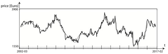
Figure 4.
The cleaned original SMP data (dotted line) vs. the noised predecessor (solid line).
The second stage of the trials was to predict the denoised data by a matched forecasting algorithm (e.g., CNN, ANN, ARIMA, or LSSVR). Furthermore, some benchmark procedures, including standalone and fusion prediction algorithms, were verified. Each test run was repeated 100 times in order to generate statistically meaningful quality measures. For all the below-listed forecasting algorithms, the statistical analysis was evaluated using the mean and the standard deviation (std).
It has been shown that all the p-values are less than 0.01, which means that there is a significant difference between the presented algorithm and the other algorithms.
The robustness of Compressed Sensing-based denoising in enhancing prediction performance is detailed in the following tables. Moreover, each tested prediction method was run as a native technique as well as preconditioned by several denoising procedures.
For quantitative measurement, the Dstat and RMSE metrics were also calculated.
From the performed analysis, the following conclusions are made, see Table 2, Table 3, Table 4 and Table 5. First, the presented hybrid forecasting scheme and the other artificial intelligence based hybrid techniques (i.e., CS-ANN and CS-LSSVR) provide the best results in terms of either directional or level prediction. It confirms that the presented methodology performs the best. Furthermore, the conducted trials also indicated a higher rates of one step ahead prediction, while the CS-LSSVR achieves its highest rates in the case of five steps ahead prediction. It is also clearly seen that compressed sensing based denoising technique can effectively make the used training sets noise level, and thus help in improving the prediction performance of methods. Second, when comparing the compressed-sensing based hybrid procedures with their single benchmarks equivalents, the former models mostly defeat the latter in either directional of level prediction, which once again confirms the robustness of the proposed technique in improving model prediction metrics.
Table 2.
Dstat comparisons between the presented algorithm for one step ahead forecasting cases.
Table 3.
Dstat comparisons between the presented algorithm for five step ahead forecasting cases.
Table 4.
RMSE comparisons between the presented algorithm for one step ahead forecasting cases.
Table 5.
RMSE comparisons between the presented algorithm for five step ahead forecasting cases.
Third, concentrating on forecasting methods, the CSD-AI’s (including the proposed CS-CNN scheme) perform much better than CS-denoised-ARIMA, and single artificial intelligence algorithms of LSSVR and ANN perform better that ARIMA as standalone, in either level or direction prediction, which further indicates the superiority of the proposed CSD-AI methodology with AI as forecasting tools. Additionally, Compressed-Sensing-ARIMA delivers poorer results than ARIMA in five steps ahead prediction. It can be justified by the fact that AIs are more effective in modeling of the nonlinear patterns hidden in SMP time series, while the traditional procedure may decrease its precision in the case of such complex data.
All the conclusions listed above were statistically confirmed. The tables reveal the results of these metrics, which were calculated for one- and five-step prediction cases. It can be noticed that the tested algorithms achieve higher performance metrics for one-step prediction cases than for five-step predictions.
To evaluate directional prediction accuracy, Dstat values were calculated. It is evident that the presented method outperforms all the competitors (see the tables above). Moreover, the applied denoising procedures improved performance rates in all cases.
The calculated metrics are better for one- and five-step predictions. The achieved improvement is less spectacular for five-step prediction than for the one-step one.
It was confirmed that all the artificial intelligence-based prediction methods are superior to the traditional forecasting schemes, i.e. ARIMA. This method was forced to struggle with nonlinearities which frequently affect complex patterns in SMP price data. The accuracy improvement of the algorithm obtained by preconditioning based on CS was moderated.
The conclusions are consistent with those obtained from the RMSE and Dstat analyses.
The tables above show that the calculated RMSE rates for the presented method and all other hybrid algorithms are lower than single methods. The lowest value was achieved for the algorithm presented in this paper. The CS-CNN method turned out to obtain the lowest RMSE rate.
It was proved that the applied CNN forecasting scheme learning paradigm is an efficient tool in terms of improving the prediction performance of the model by decreasing the noise level observed in the data of SMP price. Precisely for these reasons, the improved CNN methodology relies exclusively on the principle of the CS framework as the top-level denoising procedure.
The achieved p-values for all the stats are much smaller than 0.1, demonstrating the robustness of the presented method.
Moreover, concentrating on prediction methods, by comparing the Compressed-Sensing-Denoising-AI techniques (i.e., Compressed-Sensing-Denoising-ANN and Compressed-Sensing-Denoising-LSSVR) with Compressed-Sensing-Denoising-ARIMA and comparing Artificial Intelligence, Artificial Neural Networks and Least Square Support Vector Regression with Autoregressive Integrated Moving Average, all the p-values are significantly below 0.1, confirming that the Artificial Neural Networks were more accurate than the regular forecasting methods such as ARIMA in the case of SMP price dataset under the confidence level of 90%.
6. Conclusions and Future Research
The accomplished results are very promising and motivating for future research. Convolutional Neural Network models can be applied to SMP time series forecasting. Unlike other machine learning frameworks, CNNs are capable of unsupervised learning features from sequence data, support multivariate data, and can directly produce a vector for multi-step forecasting. As such, 1D CNNs have performed well and even achieved state-of-the-art results on challenging sequence prediction problems. Moreover, their performance rates depend on the relevancy of the CNN’s training sets. The CS methodology can effectively enhance the forecasting ability, since all the described here CS denoising-based prediction algorithms are better than their standalone equivalents with the CS-based filtering omitted.
It is worth being underlined that satisfying results occurred with all the above-tested hybrid models. The presented method indicated its effectiveness in expressing nonlinear patterns hidden in the SMP price. The proposed algorithm was tested and finally revealed its superiority over the others in terms of either level or directional predictions, offering its versatility and stability.
Due to the complexity of SMP price time series in terms of high noise levels, a presented CS-CNN is suggested, by combining the CSD and convolutional neural networks as the main prediction core.
In the presented scheme, compressed sensing-based denoising procedure is applied as original data preconditioner, finally making a convolutional neural network-based forecasting engine more efficient and precise.
With SMP price data of the Global Dairy Trade as sample data, the empirical trials indicated that the CSD process can drastically enhance the forecasting capability of the CNN model, since the presented method outperforms its single benchmarks as well as other state-of-the-art methods in both level and directional predictions.
Furthermore, several points concerning the future research direction related to this field can be highlighted. First, there are at least several lines of research along which future studies can be carried out: (1) The algorithm with slight modifications related to a time window width, training sets, etc. can be directly applied to numerous times series forecasting cases including wheat, poultry, rye, and even carbon emissions pricing. (2) Due to the increased enormity of the number of COVID-19 cases, the role of Artificial Intelligence (AI) is imperative in the current scenario. (3) The data pre-processing and feature extraction are supposed to be made with the real world COVID-19 dataset. (4) The presented algorithm is worth being tested for post-pandemic forecasting cases, which are yet to come.
Author Contributions
Conceptualization, J.M. and W.C.; methodology, J.M.; software, J.M.; validation, J.M. and W.C.; formal analysis, J.M.; investigation, J.M.; resources, J.M.; data curation, J.M.; writing—original draft preparation, J.M.; writing—review and editing, J.M. and W.C.; visualization, J.M.; supervision, W.C.; project administration, J.M. and W.C.; funding acquisition, W.C. Both authors have read and agreed to the published version of the manuscript.
Funding
This research received no external funding.
Institutional Review Board Statement
Not applicable.
Informed Consent Statement
Not applicable.
Data Availability Statement
Not applicable.
Conflicts of Interest
The authors declare no conflict of interest.
References
- Beghin, J. Dairy Markets in Asia. An Overview of Recent Findings and Implications; Briefing Paper 05-BP-47; Centre of Agricultural and Rural Development, Iowa State: Ames, IA, USA, 2005. [Google Scholar]
- Dong, F. The Outlook for Asian Dairy Markets: The Role of Demographics, Income, and Prices. Food Policy 2006, 31, 260–271. [Google Scholar] [CrossRef]
- Asche, F.; Bremnes, H.; Wessels, C. Product Aggregation, Market Integration, and Relationships between Prices. Am. J. Agric. Econ. 1999, 81, 568–581. [Google Scholar] [CrossRef]
- Murphy, M.D.; O’Mahony, M.J.; Shalloo, L.; French, P.; Upton, J. Comparison of modelling techniques for milk-production forecasting. J. Dairy Sci. 2014, 97, 3352–3363. [Google Scholar] [CrossRef] [PubMed]
- Smith, L.P. Forecasting annual milk yields. Agric. Meteorol. 1968, 5, 209–214. [Google Scholar] [CrossRef]
- André, G.; Berentsen, P.B.M.; Engel, B.; De Koning, C.J.A.M.; Lansink, A.O. Increasing the revenues from automatic milking by using individual variation in milking characteristics. J. Dairy Sci. 2010, 93, 942–953. [Google Scholar] [CrossRef] [PubMed]
- Van Bebber, J.; Reinsch, N.; Junge, W.; Kalm, E. Monitoring daily milk yields with a recursive test day repeatability model (Kalman filter). J. Dairy Sci. 1999, 82, 2421–2429. [Google Scholar] [CrossRef]
- Bhosale, M.D.; Singh, T.P. Development of Lifetime Milk Yield Equation Using Artificial Neural Network in Holstein Friesian Cross Breddairy Cattle and Comparison with Multiple Linear Regression Model. Curr. Sci. 2017, 113, 951–955. [Google Scholar] [CrossRef]
- Cole, J.B.; Null, D.J.; Vanraden, P.M. Best prediction of yields for long lactations. J. Dairy Sci. 2009, 92, 1796–1810. [Google Scholar] [CrossRef]
- Dongre, V.B.; Gandhi, R.S.; Singh, A.; Ruhil, A.P. Comparative efficiency of artificial neural networks and multiple linear regression analysis for prediction of first lactation 305-day milk yield in Sahiwal cattle. Livest. Sci. 2012, 147, 192–197. [Google Scholar] [CrossRef]
- Mirzaee, H. Long-term prediction of chaotic time series with multi-step prediction horizons by a neural network with Levenberg–Marquardt learning algorithm. Chaos Solitons Fractals 2009, 41, 1975–1979. [Google Scholar] [CrossRef]
- Pesaran, B.; Pesaran, M.H. Time Series Econometrics Using Microfit 5.0; Oxford University Press: New York, NY, USA, 2009. [Google Scholar]
- Gomez, V. The Use of Butterworth Filters for Trend and Cycle Estimation in Economic Time Series. J. Bus. Econ. Stat. 2001, 19, 365–373. [Google Scholar] [CrossRef]
- Schenk-Hoppe, K.R. Economic Growth and Business Cycles: A Critical Comment on Detrending Time Series. Stud. Nonlinear Dyn. Econom. 2001, 5, 75–86. [Google Scholar] [CrossRef]
- Baxter, M. Real exchange rates and real interest differentials:Have we missed the business- cycle relationship. J. Monet. Econ. 1994, 33, 5–37. [Google Scholar] [CrossRef]
- Baxter, M.; King, R.G. Measuring Business Cycles: Approximate Band-Pass Filters for Economic Time Series; Review of Economics and Statistics, No. 5022; NBER Working Papers; MIT Press: Cambridge, MA, USA, 1999; Volume 81, pp. 575–593. [Google Scholar]
- Stock, J.H.; Watson, M.W. Business Cycle Fluctuations in US Macroeconomic Time Series; Handbook of Macroeconomics, NBER Working Paper Series, No. 6528; Elsevier: Amsterdam, The Netherlands, 1998. [Google Scholar]
- Weng, Z. An R Package for Continuous Time Autoregressive Models via Kaman Filter, Cran. Available online: r-project.org/web/packages/cts/vignettes/kf.pdf (accessed on 25 May 2012).
- Kominakis, A.P.P.; Abas, Z.; Maltaris, I.; Rogdakis, E. A preliminary study of the application of artificial neural networks to prediction of milk yield in dairy sheep. Comput. Electron. Agric. 2002, 35, 35–48. [Google Scholar] [CrossRef]
- Lyons, W.B.; Fitzpatrick, C.; Flanagan, C.; Lewis, E. A novel multipoint luminescent coated ultra violet fibre sensor utilising artificial neural network pattern recognition techniques. Sens. Actuators A Phys. 2004, 115, 267–272. [Google Scholar] [CrossRef]
- Paoli, C.; Voyant, C.; Muselli, M.; Nivet, M.L. Use of Exogenous Data to Improve an Artificial Neural Networks Dedicated to Daily Global Radiation Forecasting. In Proceedings of the 2010 9th International Conference on Environment and Electrical Engineering, Prague, Czech Republic, 16–19 May 2010; pp. 49–52. [Google Scholar]
- Bao, Y.; Xiong, T.; Hu, Z. Multi step ahead time series prediction using multiple- output support vector regression. Neurocomputing 2014, 129, 482–493. [Google Scholar] [CrossRef]
- Hornik, K.; Stinchcombe, M.; White, H. Multilayer feedforward networks are universal approximators. Neural Netw. 1989, 2, 359–366. [Google Scholar] [CrossRef]
- Bao, Y.; Xiong, T.; Hu, Z. PSO-MISMO modeling strategy for multi step ahead time series prediction. IEEE Trans. Cybern. 2013, 44, 655–668. [Google Scholar]
- Medsker, L.R.; Jain, L.C. Recurrent Neural Networks: Design and Applications; CRC Press: Boca Raton, FL, USA, 2001. [Google Scholar]
- Takeuchi, L.; Lee, Y.-Y.A. Applying Deep Learning to Enhance Momentum Trading Strategies in Stocks. In Technical Report; Stanford University: Stanford, CA, USA, 2013. [Google Scholar]
- Hochreiter, S.; Schmidhuber, J. Long short-term memory. Neural Comput. 1997, 9, 1735–1780. [Google Scholar] [CrossRef]
- Pedregosa, F.; Varoquaux, G.; Gramfort, A.; Michel, V.; Thirion, B.; Grisel, O.; Blondel, M.; Prettenhofer, P.; Weiss, R.; Dubourg, V.; et al. Scikit-learn: Machine learning in python. J. Mach. Learn. Res. 2011, 12, 2825–2830. [Google Scholar]
- Zhu, Y.; Groth, O.; Bernstein, M.; Fei-Fei, L. Visual7w: Grounded Question Answering in Images. In Proceedings of the IEEE Conference on Computer Vision and Pattern Recognition, Las Vegas, NV, USA, 27–30 June 2016; pp. 4995–5004. [Google Scholar]
- Tkachenko, R.; Izonin, I. Model and Principles for the Implementation of Neural-Like Structures Based on Geometric Data Transformations. Adv. Intell. Syst. Comput. 2019. [Google Scholar] [CrossRef]
- Tkachenko, R.; Izonin, I.; Kryvinska, N.; Tkachenko, P. Multiple Linear Regression Based on Coefficients Identification Using Non-iterative SGTM Neural-like Structure. Adv. Comput. Intell. 2019. [Google Scholar] [CrossRef]
- Tkachenko, R.; Izonin, I.; Vitynskyi, P.; Lotoshynska, N.; Pavlyuk, O. Development of the Non-Iterative Supervised Learning Predictor Based on the Ito Decomposition and SGTM Neural-Like Structure for Managing Medical Insurance Costs. Data J. 2018, 3, 46. [Google Scholar] [CrossRef]
- Nasseri, M.; Moeini, A.; Tabesh, M. Forecasting monthly urban water demand using Extended Kalman Filter and Genetic Programming. Expert Syst. Appl. 2011, 38, 7387–7395. [Google Scholar] [CrossRef]
- Xie, W.; Yu, L.; Xu, S.; Wang, S. A new method for crude oil price forecasting based on support vector machines. In Computational Science—ICCS; Springer: Berlin/Heidelberg, Germany, 2006; pp. 444–451. [Google Scholar]
- Shambora, W.E.; Rossiter, R. Are there exploitable inefficiencies in the futures market for oil? Energy Econ. 2007, 29, 18–27. [Google Scholar] [CrossRef]
- Yu, L.; Lai, K.K.; Wang, S.; He, K. Oil Price Forecasting with An EMD-Based Multiscale Neural Network Learning Paradigm. In Computational Science—ICCS; Springer: Berlin/Heidelberg, Germany, 2007; pp. 925–932. [Google Scholar]
- Sang, Y.F. Improved wavelet modeling framework for hydrologic time series forecasting. Water Resour. Manag. 2011, 27, 2807–2821. [Google Scholar] [CrossRef]
- He, K.; Lai, K.K.; Yen, J. A hybrid slantlet denoising least squares support vector regression model for exchange rate prediction. Procedia Comput. Sci. 2010, 1, 2397–2405. [Google Scholar] [CrossRef]
- Faria, E.L.; Albuquerque, M.P.; Gonzalez, J.L.; Cavalcante, J.T.P.; Albuquerque, M.P. Predicting the Brazilian stock market through neural networks and adaptive exponential smoothing methods. Expert Syst. Appl. 2009, 36, 12506–12509. [Google Scholar] [CrossRef]
- Yuan, C. Forecasting exchange rates: The multi-state Markov-switching model with smoothing. Int. Rev. Econ. Financ. 2011, 20, 342–362. [Google Scholar] [CrossRef]
- Chen, B.T.; Chen, M.Y.; Fan, M.H.; Chen, C.C. Forecasting Stock Price Based on Fuzzy Time-Series with Equal-Frequency Partitioning and Fast Fourier Transform Algorithm. In Proceedings of the Computing, Communications and Applications Conference (ComComAp), Hong Kong, China, 11–13 January 2012; pp. 238–243. [Google Scholar]
- Sang, Y.F.; Wang, D.; Wu, J.C.; Zhu, Q.P.; Wang, L. Entropy-based wavelet de-noising method for time series analysis. Entropy 2009, 11, 1123–1147. [Google Scholar] [CrossRef]
- Dixon, M.F.; Klabjan, D.; Bang, J.H. Classification-based financial markets prediction using deep neural networks. Algorithmic Financ. 2016, 6, 67–77. [Google Scholar] [CrossRef]
- Rasekhschaffe, K.; Jones, R. Machine learning for stock selection. Financ. Anal. J. Forthcom. 2019, 6, 67–77. [Google Scholar] [CrossRef]
- Jin, J.; Yang, B.; Liang, K.; Wang, X. General image denoising framework based on compressive sensing theory. Comput. Graph. 2014, 38, 382–391. [Google Scholar] [CrossRef]
- Yu, Y.; Zhao, L. Tang, A compressed sensing based AI learning paradigm for crude oil price forecasting. Energy Econ. 2014, 46, 236–245. [Google Scholar] [CrossRef]
- He, Z.; Zhou, J.; Dai, H.-N.; Wang, H. Gold Price Forecast Based on LSTM-CNN Model. In Proceedings of the 2019 IEEE Intl Conf on Dependable, Autonomic and Secure Computing, Intl Conf on Pervasive Intelligence and Computing, Intl Conf on Cloud and Big Data Computing, Intl Conf on Cyber Science and Technology Congress (DASC/PiCom/CBDCom/CyberSciTech), Fukuoka, Japan, 5–8 August 2019; pp. 1046–1105. [Google Scholar]
- Yamashita, R.; Nishio, M.; Do, R.K.G.; Togashi, K. Convolutional neural networks: An overview and application in radiology. Insights Imaging 2018, 9, 611–629. [Google Scholar] [CrossRef]
- Jaswal, D.; Soman, K.P. Image classification using convolutional neural networks. Int. J. Adv. Res. Technol. 2014, 3. [Google Scholar] [CrossRef]
- Graves, A.; Mohamed, A.R.; Hinton, G. Speech recognition with deep recurrent neural networks. In Proceedings of the IEEE International Conference on Acoustics, Speech and Signal Processing (ICASSP), Vancouver, BC, Canada, 26–31 May 2013; pp. 6645–6649. [Google Scholar]
- Xu, K.; Ba, J.; Kiros, R.; Cho, K.; Courville, A.; Salakhudinov, R.; Zemel, R.; Bengio, Y. Show, Attend and Tell: Neural Image Caption Generation with Visual Attention. In Proceedings of the International Conference on Machine Learning, Lille, France, 7–9 July 2015; Volume 14, pp. 77–81. [Google Scholar]
- Mao, J.; Xu, W.; Yang, Y.; Wang, J.; Huang, Z.; Yuille, A. Deep captioning with multimodal recurrent neural networks (m-rnn). arXiv 2014, arXiv:1412.6632. [Google Scholar]
- LeCun, Y.; Bengio, Y. Convolutional Networks for Images, Speech, and Time Series. In The Handbook of Brain Theory and Neural Networks; MIT Press: Cambridge, MA, USA, 1995; Volume 3361. [Google Scholar]
- He, K.; Zhang, X.; Ren, S.; Sun, J. Deep Residual Learning for Image Recognition. In Proceedings of the IEEE Conference on Computer Vision and Pattern Recognition, Las Vegas, NV, USA, 27–30 June 2016; pp. 770–778. [Google Scholar]
- Tsantekidis, A.; Passalis, N.; Tefas, A.; Kanniainen, J.; Gabbouj, M.; Iosifidis, A. Forecasting Stock Prices from The Limit Order Book Using Convolutional Neural Networks. In Proceedings of the 2017 IEEE 19th Conference on Business Informatics (CBI), Thessaloniki, Greece, 24–27 July 2017; Volume 1, pp. 7–12. [Google Scholar]
- Rockefeller, B. Technical Analysis for Dummies, 3rd ed.; Wiley Publishing, Inc.: Hoboken, NJ, USA, 2014. [Google Scholar]
- Candès, E.J.; Wakin, M.B. An introduction to compressive sampling. IEEE Signal Process. Mag. 2008, 25, 21–30. [Google Scholar] [CrossRef]
- Eldar, Y.C.; Kutyniok, G. Compressed Sensing: Theory and Applications; Cambridge University Press: Cambridge, UK, 2012. [Google Scholar]
- Han, B.; Xiong, J.; Li, L.; Yang, J.; Wang, Z. Research on Millimeter-Wave Image Denoising Method Based on Contourlet and Compressed Sensing. In Proceedings of the 2010 2nd International Conference on Signal Processing Systems (ICSPS), Dalian, China, 5–7 July 2010; Volume 2, pp. V2-471–V2-475. [Google Scholar]
- Zhu, L.; Zhu, Y.; Mao, H.; Gu, M. A New Method for Sparse Signal Denoising Based on Compressed Sensing. In Proceedings of the Second International Symposium on Knowledge Acquisition and Modeling, Wuhan, China, 30 November–1 December 2009; pp. 35–38. [Google Scholar]
- Xu, B.; Wang, N.; Chen, T.; Li, M. Empirical evaluation of rectified activations in convolutional network. arXiv 2015, arXiv:1505.00853. [Google Scholar]
- Box, G.E.P.; Jenkins, G.M. Time Series Analysis: Forecasting and Control; Holden Day Press: San Francisco, CA, USA, 1970. [Google Scholar]
- Ahmed, N.; Natarajan, T.; Rao, K.R. Discrete cosine transform. IEEE Trans. Comput. 1974, 100, 90–93. [Google Scholar] [CrossRef]


Publisher’s Note: MDPI stays neutral with regard to jurisdictional claims in published maps and institutional affiliations. |
© 2021 by the authors. Licensee MDPI, Basel, Switzerland. This article is an open access article distributed under the terms and conditions of the Creative Commons Attribution (CC BY) license (http://creativecommons.org/licenses/by/4.0/).