
The Role of Energy and Environmental Quality in Exploring the Economic Sustainability: A New Appraisal in the Context of North African Countries


Abstract
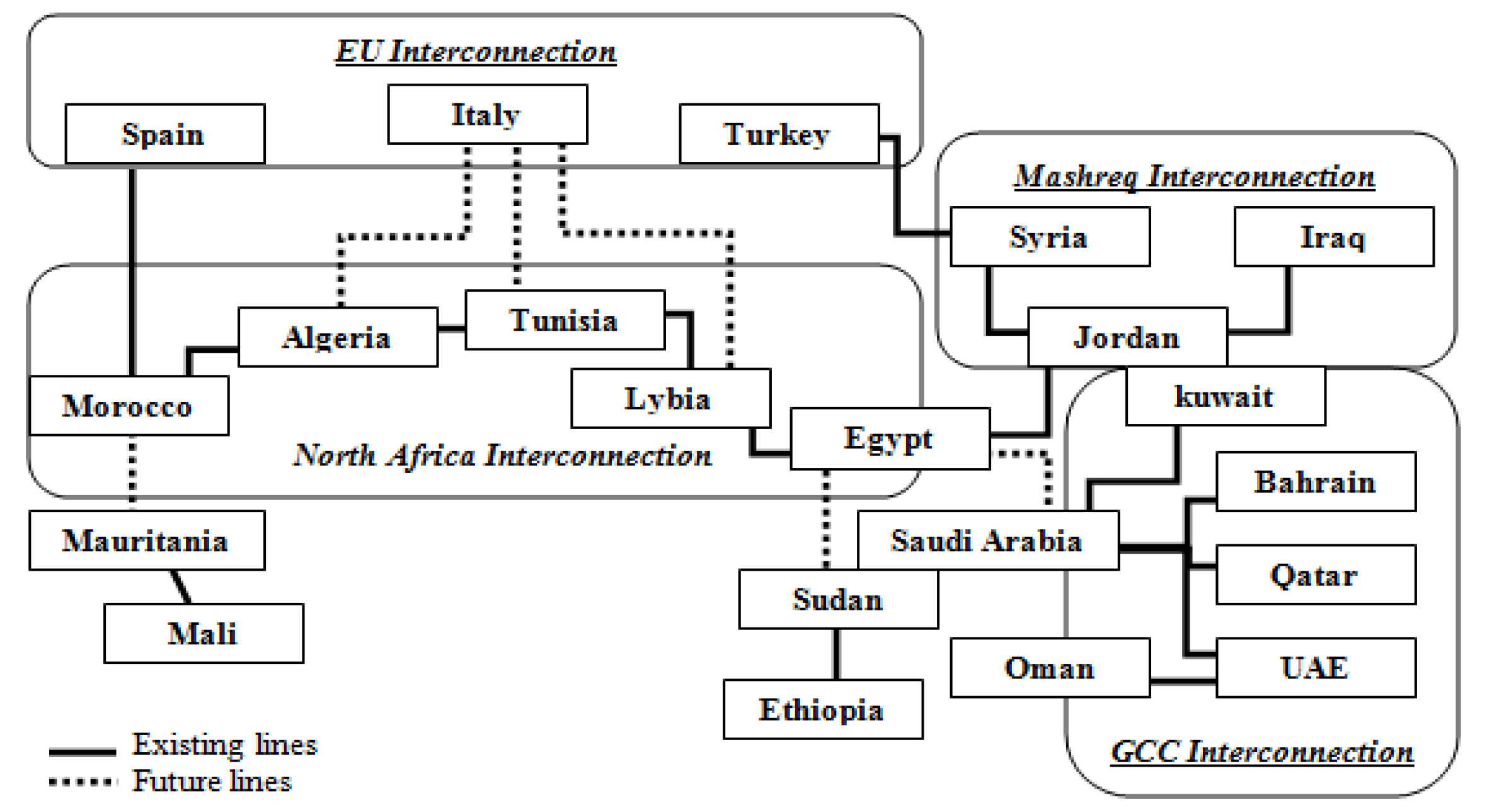
:1. Introduction
2. Literature Review
3. Data and Empirical Methodology
3.1. Data
3.2. Econometric Methodology
3.2.1. Panel Unit Root Tests
3.2.2. Panel Cointegration Tests
3.2.3. FMOLS, DOLS and PMG Estimates
4. Econometric Results and Interpretations
5. Conclusions and Policy Implications
Author Contributions
Funding
Data Availability Statement
Conflicts of Interest
References
- Alagidede, P.; Adu, G.; Frimpong, P.B. The Effect of Climate Change on Economic Growth: Evidence from Sub-Saharan Africa. Environ. Sci. Pollut. Res. 2016, 18, 417–436. [Google Scholar] [CrossRef] [Green Version]
- Ang, J.B. CO2 Emissions, Energy Consumption, and Output in France. Energy Policy 2007, 35, 4772–4778. [Google Scholar] [CrossRef]
- Arouri, M.H.; Ben Youssef, A.; M’Henni, H.; Rault, C. Energy Consumption, Economic Growth and CO2 Emissions in Middle East and North African Countries. Energy Policy 2012, 45, 342–349. [Google Scholar] [CrossRef] [Green Version]
- Gardiner, R.; Hajek, P. Interactions among Energy Consumption, CO2, and Economic Development in European Union Countries. Sustain. Dev. 2020, 28, 723–740. [Google Scholar] [CrossRef]
- Soytas, U.; Sari, R.; Ewing, B.T. Energy Consumption, Income, and Carbon Emissions in the United States. Ecol. Econ. 2007, 62, 482–489. [Google Scholar] [CrossRef]
- Aye, G.C.; Edoja, P.E. Effect of Economic Growth on CO2 Emission in Developing Countries: Evidence from a Dynamic Panel Threshold Model. Cogent Econ. Financ. 2017, 5, 1–22. [Google Scholar] [CrossRef]
- World Bank Development Report (WDR). Energy Sector Management Assistance Program: Potentials of Energy Integration in Mashreq and Neighboring Countries; World Bank Development Report: Washington, DC, USA, 2010. [Google Scholar]
- Ahmed, S.M.; Dougherty, W. Climate Change and the Environment. In Unlocking North Africa’s Potential through Regional Integration: Challenges and Opportunities; Santi, E., Ben Romdhane, S., Shaw, W., Eds.; African Development Bank (AfDB) Group, Temporary Relocation Agency (TRA): Tunis-Belvedere, Tunisia, 2012. [Google Scholar]
- Coondoo, D.; Dinda, S. Causality between Income and Emission: A Country Group Specific Econometric Analysis. Ecol. Econ. 2002, 40, 351–367. [Google Scholar] [CrossRef]
- Hamilton, C.; Turton, H. Determinants of Emissions Growth in OECD Countries. Energy Policy 2002, 30, 63–71. [Google Scholar] [CrossRef]
- Liu, X. Explaining the Relationship between CO2 Emissions and National Income—The Role of Energy Consumption. Econ. Lett. 2005, 87, 325–328. [Google Scholar] [CrossRef]
- Richmond, A.K.; Kaufmann, R.K. Is There a Turning Point in the Relationship between Income and Energy Use and/or Carbon Emissions? Ecol. Econ. 2006, 56, 176–189. [Google Scholar] [CrossRef]
- Huang, B.N.; Hwang, M.J.; Yang, C.W. Causal Relationship between Energy Consumption and GDP Growth Revisited: A Dynamic Panel Data Approach. Ecol. Econ. 2008, 67, 41–54. [Google Scholar] [CrossRef]
- Apergis, N.; Payne, J.E. CO2 Emissions, Energy Usage and Output in Central America. Energy Policy 2009, 37, 3282–3286. [Google Scholar] [CrossRef]
- Akbostanci, E.; Türüt-Aşik, S.; Tunç, G.I. The Relationship between Income and Environment in Turkey: Is There an Environmental Kuznets Curve? Energy Policy 2009, 37, 861–867. [Google Scholar] [CrossRef]
- Soytas, U.; Sari, R. Energy Consumption, Economic Growth, and Carbon Emissions: Challenges Faced by an EU Candidate Member. Ecol. Econ. 2009, 68, 1667–1675. [Google Scholar] [CrossRef]
- Ozturk, I.; Acaravci, A. CO2 Emissions, Energy Consumption and Economic Growth in Turkey. Renew. Sustain. Energy Rev. 2010, 14, 3220–3225. [Google Scholar] [CrossRef]
- Zhang, X.P.; Cheng, X.M. Energy Consumption, Carbon Emissions, and Economic Growth in China. Ecol. Econ. 2009, 68, 2706–2712. [Google Scholar] [CrossRef]
- Chang, C.C. A Multivariate Causality Test of Carbon Dioxide Emissions, Energy Consumption and Economic Growth in China. Appl. Energy 2010, 87, 3533–3537. [Google Scholar] [CrossRef]
- Acaravci, A.; Ozturk, I. On the Relationship between Energy Consumption, CO2 Emissions and Economic Growth in Europe. Energy 2010, 35, 5412–5420. [Google Scholar] [CrossRef]
- Apergis, N.; Payne, J.E. The Emissions, Energy Consumption, and Growth Nexus: Evidence from the Commonwealth of Independent States. Energy Policy 2010, 38, 650–655. [Google Scholar] [CrossRef]
- Fodha, M.; Zaghdoud, O. Economic Growth and Pollutant Emissions in Tunisia: An Empirical Analysis of the Environmental Kuznets Curve. Energy Policy 2010, 38, 1150–1156. [Google Scholar] [CrossRef]
- Narayan, P.K.; Narayan, S. Carbon Dioxide Emissions and Economic Growth: Panel Data Evidence from Developing Countries. Energy Policy 2010, 38, 661–666. [Google Scholar] [CrossRef]
- Al-mulali, U. Oil Consumption, CO2 Emission and Economic Growth in MENA Countries. Energy 2011, 36, 6165–6171. [Google Scholar] [CrossRef]
- Hossain, M.S. Panel Estimation for CO2 Emissions, Energy Consumption, Economic Growth, Trade Openness and Urbanization of Newly Industrialized Countries. Energy Policy 2011, 39, 6991–6999. [Google Scholar] [CrossRef]
- Niu, S.; Ding, Y.; Niu, Y.; Li, Y.; Luo, G. Economic Growth, Energy Conservation and Emissions Reduction: A Comparative Analysis based on Panel Data for 8 Asian-Pacific Countries. Energy Policy 2011, 39, 2121–2131. [Google Scholar] [CrossRef]
- Wang, S.S.; Zhou, D.Q.; Zhou, P.; Wang, Q.W. CO2 Emissions, Energy Consumption and Economic Growth in China: A Panel Data Analysis. Energy Policy 2011, 39, 4870–4875. [Google Scholar] [CrossRef]
- Farhani, S.; Ben Rejeb, J. Energy Consumption, Economic Growth and CO2 Emissions: Evidence from Panel Data for MENA Region. Int. J. Energy Econ. Policy 2012, 2, 71–81. [Google Scholar]
- Al-mulali, U.; Che Sab, C.N.B. The Impact of Energy Consumption and CO2 Emission on the Economic Growth and Financial Development in the Sub Saharan African Countries. Energy 2012, 39, 180–186. [Google Scholar] [CrossRef]
- Shahbaz, M.; Lean, H.H.; Shabbir, M.S. Environmental Kuznets Curve hypothesis in Pakistan: Cointegration and Granger causality. Renew. Sustain. Energy Rev. 2012, 16, 2947–2953. [Google Scholar] [CrossRef] [Green Version]
- Chandran, V.G.R.; Tang, C.F. The Dynamic Links between CO2 Emissions, Economic Growth and Coal Consumption in China and India. Appl. Energy 2013, 104, 310–318. [Google Scholar] [CrossRef]
- Lim, K.-M.; Lim, S.-Y.; Yoo, S.-H. Oil Consumption, CO2 Emission, and Economic Growth: Evidence from the Philippines. Sustainability 2014, 6, 967–979. [Google Scholar] [CrossRef] [Green Version]
- Azam, M.; Khan, A.Q.; Bin Abdullah, H.; Muhammad Ejaz Qureshi, M.E. The Impact of CO2 Emissions on Economic Growth: Evidence from Selected Higher CO2 Emissions Economies. Environ. Sci. Pollut. Res. 2016, 23, 6376–6389. [Google Scholar] [CrossRef]
- Al-mulali, U.; Che Sab, C.N.B. The impact of coal consumption and CO2 emission on economic growth. Energy Sources B Econ. Plan. Policy 2018, 13, 218–223. [Google Scholar] [CrossRef]
- Bhat, J.A. Renewable and Non-renewable Energy Consumption-Impact on Economic Growth and CO2 Emissions in Five Emerging Market Economies. Environ. Sci. Pollut. Res. 2018, 25, 35515–35530. [Google Scholar] [CrossRef]
- Lin, F.-L.; Inglesi-Lotz, R.; Chang, T. Revisit Coal Consumption, CO2 Emissions and Economic Growth nexus in China and India using a Newly Developed Bootstrap ARDL Bound Test. Energy Explor. Exploit. 2018, 36, 450–463. [Google Scholar] [CrossRef] [Green Version]
- Dong, K.; Sun, R.; Li, H.; Liao, H. Does Natural Gas Consumption Mitigate CO2 Emissions: Testing the Environmental Kuznets Curve Hypothesis for 14 Asia-Pacific Countries. Renew. Sustain. Energy Rev. 2018, 94, 419–429. [Google Scholar] [CrossRef]
- Mardani, A.; Streimikiene, D.; Cavallaro, F.; Loganathan, N.; Khoshnoudi, M. Carbon Dioxide (CO2) Emissions and Economic Growth: A Systematic Review of Two Decades of Research from 1995 to 2017. Sci. Total Environ. 2019, 649, 31–49. [Google Scholar] [CrossRef] [PubMed]
- Yusuf, A.M.; Abubakar, A.B.; Mamman, S.O. Relationship between Greenhouse Gas Emission, Energy Consumption, and Economic Growth: Evidence from Some Selected Oil-Producing African Countries. Environ. Sci. Pollut. Res. 2020, 27, 15815–15823. [Google Scholar] [CrossRef] [PubMed] [Green Version]
- Islam, M.M.; Alharthi, M.; Murad, M.W. The Effects of Carbon Emissions, Rainfall, Temperature, Inflation, Population, and Unemployment on Economic Growth in Saudi Arabia: An ARDL Investigation. PLoS ONE 2021, 16, e0248743. [Google Scholar] [CrossRef] [PubMed]
- Máté, D.; Novotny, A.; Meyer, D.F. The Impact of Sustainability Goals on Productivity Growth: The Moderating Role of Global Warming. Int. J. Environ. Res. Public Health 2021, 18, 11034. [Google Scholar] [CrossRef] [PubMed]
- Levin, A.; Lin, C.F.; Chu, C.S. Unit Root Tests in Panel Data: Asymptotic and Finite-Sample Properties. J. Econom. 2002, 108, 1–24. [Google Scholar] [CrossRef]
- Im, K.S.; Pesaran, M.H.; Shin, Y. Testing for Unit Roots in Heterogeneous Panels. J. Econom. 2003, 115, 53–74. [Google Scholar] [CrossRef]
- Maddala, G.S.; Wu, S. A Comparative Study of Unit Root Tests with Panel Data and a New Simple Test. Oxf. Bull. Econ. Stat. 1999, 61, 631–652. [Google Scholar] [CrossRef]
- Hadri, K. Testing for Stationarity in Heterogeneous Panel Data. Econom. J. 2000, 3, 148–161. [Google Scholar] [CrossRef]
- Pedroni, P. Critical Values for Cointegration Tests in Heterogeneous Panels with Multiple Regressors. Oxf. Bull. Econ. Stat. 1999, 61, 653–670. [Google Scholar] [CrossRef]
- Pedroni, P. Panel Cointegration: Asymptotic and Finite Sample Properties of Pooled Time Series Tests with an Application to the PPP Hypothesis. Econom. Theory 2004, 20, 597–625. [Google Scholar] [CrossRef] [Green Version]
- Kao, C. Spurious Regression and Residual-Based Tests for Cointegration in Panel Data. J. Econom. 1999, 90, 1–44. [Google Scholar] [CrossRef]
- Dickey, D.A.; Fuller, W.A. Distribution of the Estimators for AutoRegressive Time Series with a Unit Root. J. Am. Stat. Assoc. 1979, 74, 427–431. [Google Scholar]
- Kwiatkowski, D.; Phillips, P.C.B.; Schmidt, P.; Shin, Y. Testing the Null Hypothesis of Stationarity Against the Alternative of a Unit Root: How Sure Are We That Economic Time Series Have a Unit Root? J. Econom. 1992, 54, 159–178. [Google Scholar] [CrossRef]
- Engle, R.F.; Granger, C.W.J. Co-integration and Error Correction: Representation, Estimation, and Testing. Econometrica 1987, 55, 251–276. [Google Scholar] [CrossRef]
- Farhani, S.; Ben Rejeb, J. Link between Economic Growth and Energy Consumption in over 90 Countries. Interdis. J. Contem. Res. Bus. 2012, 3, 282–297. [Google Scholar]
- Phillips, P.C.B.; Perron, P. Testing for a Unit Root in Time Series Regressions. Biometrika 1988, 75, 335–346. [Google Scholar] [CrossRef]
- Pedroni, P. Fully Modified OLS for Heterogeneous Cointegrated Panels. In Advances in Econometrics: Nonstationary Panels, Panel Cointegration, and Dynamic Panels; Baltagi, B.H., Fomby, T.B., Hill, R.C., Eds.; Emerald Group Publishing Ltd.: Bingley, UK, 2001; Volume 15, pp. 93–130. [Google Scholar]
- Pedroni, P. Purchasing Power Parity Tests in Cointegrated Panels. Rev. Econ. Stat. 2001, 83, 727–731. [Google Scholar] [CrossRef] [Green Version]
- Kao, C.; Chiang, M.H. On the Estimation and Inference of a Cointegrated Regression in Panel Data. In Advances in Econometrics: Nonstationary Panels, Panel Cointegration, and Dynamic Panels; Baltagi, B.H., Fomby, T.B., Hill, R.C., Eds.; Emerald Group Publishing Ltd.: Bingley, UK, 2001; Volume 15, pp. 179–222. [Google Scholar]
- Phillips, P.C.B.; Hansen, B.E. Statistical Inference in Instrumental Variables Regression with I(1) Processes. Rev. Econ. Stud. 1990, 57, 99–125. [Google Scholar] [CrossRef]
- Saikkonen, P. Asymptotically Efficient Estimation of Cointegration Regressions. Econom. Theory 1991, 7, 1–21. [Google Scholar] [CrossRef]
- Stock, J.H.; Watson, M.W. A Simple Estimator of Cointegrating Vectors in Higher Order Integrated Systems. Econometrica 1993, 61, 783–820. [Google Scholar] [CrossRef]
- Phillips, P.C.B.; Moon, H.R. Linear Regression Limit Theory for Nonstationary Panel Data. Econometrica 1999, 67, 1057–1112. [Google Scholar] [CrossRef] [Green Version]
- Pesaran, M.H.; Shin, Y.; Smith, R.P. Pooled Mean Group Estimation of Dynamic Heterogeneous Panels. J. Am. Stat. Assoc. 1999, 94, 621–634. [Google Scholar] [CrossRef]
- Mark, N.C.; Sul, D. Cointegration Vector Estimation by Panel DOLS and Long-run Money Demand. Oxf. Bull. Econ. Stat. 2003, 65, 655–680. [Google Scholar] [CrossRef] [Green Version]
- Fisher, R. Statistical Methods for Research Workers; Oliver & Boyd: Edinburgh, UK, 1932. [Google Scholar]
- Ozturk, I.; Aslan, A.; Kalyoncu, H. Energy Consumption and Economic Growth Relationship: Evidence from Panel Data for Low and Middle Income Countries. Energy Policy 2010, 38, 4422–4428. [Google Scholar] [CrossRef]
- Lee, C.C.; Chang, C.P.; Chen, P.F. Energy–Income Causality in OECD Countries Revisited: The Key Role of Capital Stock. Energy Econ. 2008, 30, 2359–2373. [Google Scholar] [CrossRef]
- Lee, C.C. Energy Consumption and GDP in Developing Countries: A Cointegrated Panel Analysis. Energy Econ. 2005, 27, 415–427. [Google Scholar] [CrossRef]
- Narayan, P.K.; Smyth, R. Energy Consumption and Real GDP in G7 Countries: New Evidence from Panel Cointegration with Structural Breaks. Energy Econ. 2008, 30, 2331–2341. [Google Scholar] [CrossRef]
- Lee, C.C.; Chang, C.P. Energy Consumption and GDP Revisited: A panel Analysis of Developed and Developing Countries. Energy Econ. 2007, 29, 1206–1223. [Google Scholar] [CrossRef]
- Lee, C.C.; Chang, C.P. Energy Consumption and Economic Growth in Asian Economies: A More Comprehensive Analysis using Panel Data. Resour. Energy Econ. 2008, 30, 50–65. [Google Scholar] [CrossRef]
- Ozturk, I. A Literature Survey on Energy-Growth Nexus. Energy Policy 2010, 38, 340–349. [Google Scholar] [CrossRef]

| LNGDP | LNEC | LNCO2 | |
|---|---|---|---|
| Mean | 7.997949 | 6.612999 | 0.845502 |
| Median | 7.984966 | 6.562463 | 0.776946 |
| Maximum | 9.398046 | 8.117768 | 2.302338 |
| Minimum | 6.610536 | 5.196845 | −0.729667 |
| Std. Dev. | 0.643226 | 0.737948 | 0.771590 |
| Skewness | 0.188839 | 0.409725 | 0.352818 |
| Kurtosis | 2.437432 | 2.437763 | 2.316229 |
| Jarque-Bera | 4.591235 | 9.876092 | 9.654640 |
| Probability | 0.100699 | 0.007169 | 0.008008 |
| Sum | 1919.508 | 1587.120 | 202.9205 |
| Sum Sq. Dev. | 98.88363 | 130.1515 | 142.2889 |
| Observations | 220 | 220 | 220 |
| Cross sections | 5 | 5 | 5 |
| Method | LNGDP | LNEC | LNCO2 | |
|---|---|---|---|---|
| LLC t * | ||||
| (a) Level | (with trend) | 0.76317 (0.7773) | −1.87004 (0.0307) ** | −0.99203 (0.1606) |
| (without trend) | −1.83406 (0.0333) ** | −5.00237 (0.0000) ** | −3.93438 (0.0000) ** | |
| (b) First difference | (with trend) | −2.32732 (0.0100) ** | −6.77214 (0.0000) ** | −8.17930 (0.0000) ** |
| (without trend) | −2.57578 (0.0050) ** | −6.60241 (0.0000) ** | −8.32372 (0.0000) ** | |
| IPS W-stat | ||||
| (a) Level | (with trend) | 0.40906 (0.6588) | −0.78619 (0.2159) | −2.30766 (0.0105) ** |
| (without trend) | −0.18025 (0.4285) | −3.09734 (0.0010) ** | −2.70883 (0.0034) ** | |
| (b) First difference | (with trend) | −5.99199 (0.0000) ** | −8.47429 (0.0000) ** | −9.83138 (0.0000) ** |
| (without trend) | −6.79125 (0.0000) ** | −7.93134 (0.0000) ** | −10.1512 (0.0000) ** | |
| MW Fisher-Chi-square | ||||
| (a) Level | (with trend) | 9.45382 (0.4896) | −11.9570 (0.2879) * | 22.3713 (0.0133) ** |
| (without trend) | 15.8019 (0.1054) | −35.4562 (0.0010) ** | 23.7616 (0.0083) ** | |
| (b) First difference | (with trend) | 53.9304 (0.0000) ** | 77.8957 (0.0000) ** | 93.0935 (0.0000) ** |
| (without trend) | 66.2480 (0.0000) ** | 78.3385 (0.0000) ** | 105.125 (0.0000) ** | |
| Hadri Z-stat | ||||
| (a) Level | (with trend) | −3.20294 (0.0007) ** | −6.01093 (0.0000) ** | −4.11983 (0.0000) ** |
| (without trend) | −10.0737 (0.0000) ** | −9.69801 (0.0000) ** | −10.2798 (0.0000) ** | |
| (b) First difference | (with trend) | −1.46795 (0.0711) * | −2.97203 (0.0015) ** | −1.57339 (0.0000) ** |
| (without trend) | −0.85204 (0.1971) | −5.79565 (0.0000) ** | −0.35142 (0.3626) | |
| Method | Statistic Test | Prob | Method | Statistic Test | Prob |
|---|---|---|---|---|---|
| Within-Dimension | Between-Dimension | ||||
| Panel υ-stat | 2.197592 | 0.0140 ** | |||
| Panel r-stat | −3.000778 | 0.0013 ** | Group r-stat | −1.830518 | 0.0336 ** |
| Panel PP-stat | −3.195549 | 0.0007 ** | Group PP-stat | −2.626453 | 0.0043 ** |
| Panel ADF-stat | −1.304750 | 0.0960 | Group ADF-stat | 0.697912 | 0.7574 |
| Method | Statistic Test | Prob |
|---|---|---|
| ADF | −4.427797 ** | 0.0000 |
| Country | LNEC | LNCO2 | ||||
|---|---|---|---|---|---|---|
| FMOLS | DOLS | PMG | FMOLS | DOLS | PMG | |
| Egypt | 0.302882 ** | 0.217838 ** | 0.398099 ** | 0.668412 ** | 0.744884 ** | 0.564195 ** |
| Libya | 0.488978 ** | 0.311123 * | 0.560619 ** | −0.016155 | 0.035853 | −0.068542 |
| Tunisia | 1.900196 ** | 2.053885 ** | 1.623900 ** | −0.854048 ** | −1.025748 ** | −0.584337 ** |
| Algeria | 0.311024 ** | 0.414824 ** | 0.269849 ** | −0.057916 | −0.022819 | 0.063728 |
| Morocco | 1.179060 ** | 1.166619 ** | 1.112170 ** | −0.121162 | −0.115239 | −0.073349 |
| Panel | 1.242549 ** | 1.249666 ** | 1.237309 ** | −0.337334 ** | −0.392698 ** | −0.361694 ** |
Publisher’s Note: MDPI stays neutral with regard to jurisdictional claims in published maps and institutional affiliations. |
© 2021 by the authors. Licensee MDPI, Basel, Switzerland. This article is an open access article distributed under the terms and conditions of the Creative Commons Attribution (CC BY) license (https://creativecommons.org/licenses/by/4.0/).
Share and Cite
Farhani, S.; Kadria, M.; Guirat, Y. The Role of Energy and Environmental Quality in Exploring the Economic Sustainability: A New Appraisal in the Context of North African Countries. Sustainability 2021, 13, 13990. https://doi.org/10.3390/su132413990
Farhani S, Kadria M, Guirat Y. The Role of Energy and Environmental Quality in Exploring the Economic Sustainability: A New Appraisal in the Context of North African Countries. Sustainability. 2021; 13(24):13990. https://doi.org/10.3390/su132413990
Chicago/Turabian StyleFarhani, Sahbi, Mohamed Kadria, and Yosr Guirat. 2021. "The Role of Energy and Environmental Quality in Exploring the Economic Sustainability: A New Appraisal in the Context of North African Countries" Sustainability 13, no. 24: 13990. https://doi.org/10.3390/su132413990
APA StyleFarhani, S., Kadria, M., & Guirat, Y. (2021). The Role of Energy and Environmental Quality in Exploring the Economic Sustainability: A New Appraisal in the Context of North African Countries. Sustainability, 13(24), 13990. https://doi.org/10.3390/su132413990