Abstract
In this paper, we propose an improved cellular automaton model for the traffic operation characteristics of variable direction lanes in an Intelligent Vehicle Infrastructure Cooperation System (I-VICS). According to the proposed flow of variable oriented lane operation in the I-VICS environment, the idea for the improved model has been determined. According to an analysis of different signal states, an improved STCA model is proposed, in combination with the speed induction method of I-VICS and the variable direction lane switching strategy. In the assumed regular simulation environment, the STCA and STCA-V models are simulated under different vehicular densities. The results indicated that traffic parameters such as traffic flow and average speed of the variable direction lanes in the I-VICS environment are better than those in the conventional environment according to the operating rules of the proposed model. Moreover, lane utilization increased for the same density.
1. Introduction
Variable direction lanes have become a frequent and innovative management tool used by traffic managers to address the congestion problems caused by the tide of turning traffic in China. On Chinese urban roads, the transformation of lane function is mainly used to achieve the transfer of traffic flow. It is a highly targeted control tool for turning tidal traffic to improve the efficiency of road traffic [1,2,3]. However, during the process, some drivers are unable to obtain effective information in time, generating problems such as lane-changing decision errors and low lane utilization.
At the same time, with the road as a vehicle carrier, the I-VICS uses advanced wireless communication technology and sensing detection technology. The purpose of I-VICS is to obtain data from vehicle-to-vehicle (V2V), vehicle-to-infrastructure (V2I) sensing devices, and other related information to realize the fusion of heterogeneous data from multi-source, as well as to share the information to achieve reasonable speed and lane-changing behavior suggestions during vehicle operation so that viatic traffic can develop regarding intelligence, networking, and automation [4,5,6]. Therefore, in the I-VICS environment, more effective information can be transmitted to the driver to improve the correctness and systematization of driving decisions, especially in dynamic traffic control.
Many researchers have published predictive studies concerning the impact of I-VICS technology on road safety problems, traffic congestion, and traffic flow. Some research centers have already published studies showing that the use of connected car technology and autonomous driving would significantly reduce the number of accidents caused by driver error and reduce traffic congestion [7]. But this is a simplistic, idealistic assumption. In response, some view the assumption of accident avoidance after the introduction of I-VICS technology from the perspective of traffic flow composition. They argue that the transitional phase must exist and that traffic flow is a mixture of communicating and non-communicating vehicles [8,9,10]. This is a necessary stage in the development of intelligent transport systems (ITS). Only when the proportion of connected vehicles in the mixed traffic flow reaches a high level [11,12] will the current traffic situation be greatly improved and the probability of traffic accidents be reduced. Consequently, the current attitude is optimistic concerning the effect of I-VICS technology when fully implemented along with its impact on various traffic problems.
It has also been shown that I-VICS technology can provide comprehensive driving assistance information [13,14] and improve the ability to cope with uncertainties in the driving environment, such as adverse weather conditions, unexpected traffic events, or accidents [15,16]. But it also has disadvantages. As the driver’s behavior is mainly dependent on the perception of information and judgment of the surrounding environment, the information provided by the I-VICS system will distract the driver and affect operations [17]. Thus, it is important to minimize the impact as much as possible to truly improve the system’s reliability.
At the same time, facing the trend towards sustainable transport development, many studies are exploring the application of this technology to various intersections and roads. On the one hand, it will reduce the fuel consumption and emissions of moving vehicles, reduce environmental impact [18,19], and improve driver satisfaction. Indirectly, it will prevent incorrect driving maneuvers caused by driver emotional instability due to queuing or traffic blockage [20]. It also shows that the development of I-VICS technology has more advantages than disadvantages for the driver, the vehicle, and even the entire traffic environment.
To address the traffic flow characteristics in different scenarios under I-VICS, the construction of suitable traffic flow models can provide a reference for further research in this field. Therefore, in addition to traffic flow models such as intelligent driving models (IDM) [21], full velocity difference models (FVDM) [22], and Lighthill–Whitham–Richards (LWR) kinematic wave traffic flow model [23], Cellular Automaton (CA) is also considered to be a new kinematic model for the study of traffic flow. It has been widely used in traffic flow studies because of its accessibility and accuracy in reflecting the characteristics of traffic flow [24]. Under conventional traffic conditions, many scholars have proposed various types of CA models according to actual demands. Knospe has proposed a model that considers driver comfort driving (CD), also known as the brake light (BL) model due to its impact on the rear vehicle by introducing brake lights [25,26]. Based on this, Jiang and Wu developed an improved CD (MCD) model [27]. And Wang et al. proposed the CA model for a congestion flow (CACF) model based on the symmetric two-lane CA (STCA) model for traffic jam conditions caused by traffic accidents [28]. Some have proposed the A-STCA model for aggressive lane-changing behavior [29], the H-STCA model concerning vehicle honking [30], and the T-STCA model regarding vehicle turn signals [31]. From the above, it can be seen that there are numerous research results for traffic flow models based on the CA model, designed for different scenarios and different demands in the traditional traffic environment.
The rapid development of ITS in recent years has raised new challenges for the research of traffic flow characterization. I-VICS is still within the traffic category, and we can also regard it as a scenario that corresponds to the traditional traffic environment. The only difference is in the intelligence of control and determination. Therefore, corresponding traffic simulation experiments are essential. Due to the difficulty of reproducing the various scenarios of vehicle operation in the I-VICS environment, some have developed simulation models of traffic flow. Xiang et al. proposed the BL-STCA model for dynamic lane changes [32]. Ye et al. then simulated the characteristics of mixed traffic flow based on the two-state safe-speed Model (TSM) to study its evolution process. It was demonstrated that with the penetration of CAV, traffic safety would be improved [9,33]. Li et al. introduced guided vehicle speed and safety distance and proposed an STCA-S model based on the background of I-VICS technology [34]. However, regarding the characteristics of turning traffic flow and the corresponding driver’s lane change behavior in the I-VICS environment, there are gaps in the above studies.
The main contributions of this paper are summarised as follows:
- The operational process of variable direction lanes in the I-VICS environment is proposed, and its steps are analyzed, which aims to provide a reference for the study of variable direction lane settings in this environment.
- An improved CA model and its motion update rules are proposed, that combine the characteristics of I-VICS technology and variable guided lane control strategies. It will establish the theoretical basis for later analysis of traffic flow characterization.
- The proposed model is simulated numerically, and the traffic flow parameter curves for different density conditions and the Spatio-temporal characteristics of different CA models for maximum density are plotted. This will obtain the characteristics of the traffic flow distribution in this case. It also provides a certain theoretical basis for the construction of intelligent traffic development.
Our work is presented as follows. The Section 2 introduces the related work of the classical CA model, the installation method, and the problems of variable direction lanes in the traditional environment. The operational process of variable direction lanes in the I-VICS environment is analyzed. The Section 3 mainly addresses the assumed initial environment of the CA simulation and the main rules and motion update rules of the proposed improved model. The Section 4 mainly focuses on constructing the experimental environment and the numerical simulation and analysis from the perspective of traffic flow parameters and Spatio-temporal characteristics analysis. Finally, in Section 5, we conclude our paper and outline future research.
2. Related Work
2.1. Installations of Variable Direction Lanes and Problems Description
The setting of variable direction lanes at intersections is shown in Figure 1. The conversion process of lane attributes is analyzed as follows: the initial attributes of the variable direction lanes are set to straight ahead, i.e., the functional structure of the lanes in the drainage area is “1 left, 2 straight, 1 right”. When there is an obvious secondary queue of left-turning traffic and the straight lane is empty, the attributes of the variable direction lanes are converted to left-turning to increase the capacity of the left-turning lanes to achieve a balance between supply and demand of different turning traffic.
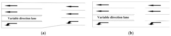
Figure 1.
Schematic diagram of the variable direction lane set-up: (a) without spreading section, (b) with spreading section.
First, in the single-lane driving environment, elements such as people, vehicles, roads, and the environment interact with each other to control the operation of the vehicle, after obtaining appropriate information through the driver’s senses and driving the vehicle concerning only the vehicles to the front and rear.
When the number of lanes is increased and variable direction lanes are installed, mutual blockage between vehicles will affect the driver’s judgment [35] and limit access to traffic information [36], resulting in different degrees of error in operational decisions such as acceleration, deceleration, and lane changing. And according to research statistics [37], about 90% of traffic accidents are caused by the aforementioned driver misjudgments and mishandling [38,39]. These errors not only increase the danger of driving but also reduce utilization of the lane. As shown in Figure 2, according to the actual survey, the main problems of the variable direction lanes at intersections are broad and as follows:
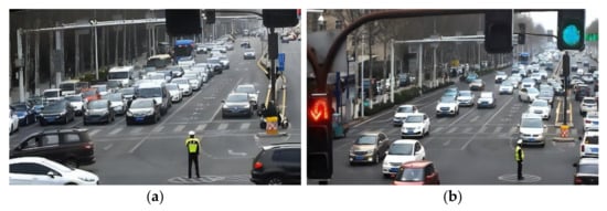
Figure 2.
Problems with Variable direction Lanes: (a) Variable direction lane emptying, (b) Driver misses lane change.
- Because of obstructing vehicles ahead or to the side, especially large vehicles such as buses or lorries, drivers cannot obtain attributes of variable direction lanes and the information about changing lanes in time, and miss the best time to change lanes.
- As shown in Figure 2a, there is a phenomenon that a single flow direction is an empty release, while the other flow direction cannot change lanes due to signal restrictions and queues.
- The switching timing attributes of variable direction lanes is difficult to determine precisely. It is usually necessary to switch ahead during the initial 2–3 signal cycles of traffic reaching the intersection, and after an adaptive period of 1–2 signal cycles. This ensures that traffic flows smoothly through the intersection [40].
- As shown in Figure 2b, there is difficulty changing lanes for vehicles in variable direction lanes when switching periods approach. Drivers need to judge whether to move into the lane based on the guidance lights. When the demand of the flow does not correspond to the function of the switched lane, vehicles need to change lanes. However, the closed lane creates bottlenecks, making it difficult for vehicles to change lanes. This aggravates the phenomenon of queue jumping and dangerous lane changes, which causes a surge in safety hazards and traffic congestion problems.
As a result, the utilization of the variable direction lane at the intersection is low, with 65.16% and 38.2% of the lanes utilized when the attributes are straight ahead and left-turning, respectively.
2.2. Operational Analysis of Variable Direction Lanes under I-VICS
- Technological advantages: The I-VICS technology provides solutions to the problems described above. Compared with the traditional environment, the vehicles in the I-VICS environment obtain driving guidance information through in-vehicle intelligent devices, which are not limited by the field of view in the actual traffic environment and can obtain status information of vehicles in a greater range. The status information includes the environment surrounding the current vehicle and the vehicles in the scope of perturbation.
- Analysis of traffic characteristics: The traffic flow models are mainly divided into two categories, macro and micro [41,42], and the propagation characteristics can also be revealed from these two perspectives. It has been found that [43] the traffic flow at the macro-level is highly random and volatile, and the global vehicle status can be grasped in real-time through the I-VICS. At the micro-level, the local vehicular traffic flow will also be transmitted in the form of traffic waves, and by providing real-time lane-changing guidance information and velocity-induced information the vehicles can be controlled to drive into or out of the variable direction lane. Therefore, the I-VICS can rely on the acquisition of global vehicle status to reduce the frequency of blind acceleration and deceleration and emergency braking to ensure the smoothness of the roads and the safety and efficiency of vehicle operation.
- Detailed operational process analysis of variable direction lanes under I-VICS:When vehicles approach the transition section from the interweave section, the roadside unit (RSU) interacts with the onboard unit (OBU) to collect vehicle status information and uses the vehicle detector to count the traffic flow data, which is uploaded to the Traffic Management Center (TMC). The message is sent to the Traffic Condition Analysis and Control (TCAC) unit for evaluation and to the TMC for processing. Finally, the message is sent to each OBU user by the RSU. Therefore, the driver can receive the message from the RSU even if he cannot see the variable message board (VMS) in positions 1 or 5. When vehicles continue to move into the analyzed area, the TCAC unit evaluates the traffic conditions in each lane of the analyzed area. At this time, it is necessary to decide whether to switch the variable direction lane (VDL) function in the following cases:
- (1)
- Attribute of the VDL switching from left-turning to straight ahead.
- When there is no left-turning queue in the VDL and the end of the straight-ahead queue is in position 6, the lane function can be switched directly.
- When the left-turning vehicles are lined up in positions 4 and 5, and the straight traffic is queued up in position 9, the VDL is first closed and the left-turning vehicles in the lane are moved away. Finally, straight-ahead traffic is guided into the lane that is re-opened.
- (2)
- Attribute of the VDL switching from straight ahead to left-turning.
- When there is no straight queue in the VDL and the end of the left-turning queue is in position 4, the lane function can be switched directly.
- When the straight vehicles are lined up in positions 5 and 6, and position 7 for left-turning traffic, the VDL is closed and cleared before opening and introducing the left-turning traffic.
The RSU also sends behavioral guidance messages to the nearest vehicle on the advice of the TCAC, such as speed and lane changes, and alerts the driver with images, sounds, or vibrations. At this moment, dedicated short-range communication (DSRC) is also used to transmit the information to the vehicle behind and guide the driver to change lanes. The above noted is a complete set of operational processes for VDLs under I-VICS. The operational analysis is shown in Figure 3.
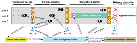
Figure 3.
Operation analysis diagram of variable direction lane under I-VICS.
3. Modelling
As the STCA model is only suitable for the conventional traffic environment, the technical characteristics of I-VICS and the operation of variable guided lanes have not been considered. The purpose of this section is based on the STCA model to construct a new CA model, which will enable better comprehension of traffic flow characteristics in this context and provide a reference for subsequent studies. According to the lane-changing rules of the STCA model in the traditional traffic environment, the vehicle lane-changing needs to satisfy both lane-changing motivation and safety conditions, while the control logic of variable direction lanes determines the lane attributes using the queue length of each turning convoy. Therefore, combining the velocity guidance function of vehicle-infrastructure cooperative and the control strategy of variable direction lanes, this paper proposes an improved STCA model, shortened to STCA-V (STCA for variable direction lane in I-VICS).
3.1. Analysis of Lane-Changing Model Based on Cellular Expression
The analysis in Section 2.2 shows the impact of the fusion of heterogeneous data from multi-sources and the interaction of information in an I-VICS environment, which provides traffic participants with certain reference value guidance information. The reasonable and effective variable direction lane changing rules will impact the utilization of road resources and the safe operation of vehicles.
The research environment is described to facilitate the analysis of the operation of available direction lanes in an I-VICS environment [44]. As shown in Figure 4, the road is considered as a 3-row discrete mesh consisting of clength cells with 1 variable and 2 fixed lanes. The direction of the vehicle is from left to right, and each number or letter indicates that the cell is occupied by a vehicle. The number and the letter indicate the speed and the code of the occupied vehicle, respectively.
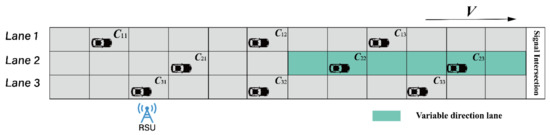
Figure 4.
Schematic diagram of the three-lane vehicle relationship.
In Figure 4, Ci,j is used to denote the jth vehicle in the ith lane, corresponding to xi,j(t), vi,j(t) and denoting the position, velocity, and spacing, respectively, between the front of vehicle Ci and the rear of vehicle Ci−1 at time t; vmax is the maximum restricted speed of the road section, and the variable range of the speed is [0, vmax]; prd is the random slowing probability that can characterize the slowing down condition of vehicles due to other traffic incidents, forming the phenomenon of blocking. Regarding vehicle movement, each vehicle will interact with the message between OBU and RSU every moment to obtain the speed and current position of other vehicles. According to the above information and the corresponding simulation operation rules, the position distribution of the next moment is derived. Furthermore, the vehicle will be disturbed by the surrounding environment while driving. Taking the position of vehicle Ci,j at moment t as the reference point in Figure 4, the vehicle relationship expression and the operating environment are set as follows:
- Assuming that the left-turning and the straight-ahead converge and release in the same phase.
- According to the standards of I-VICS [45], we decided to conduct experiments under an ideal condition of the I-VICS environment. Assuming that the OBU is within the communication range of the RSU with signal interaction frequency ≤ 1 Hz and system delay ≤ 500 ms.
- Assuming that the relationships are expressed for the three-lane traffic environment as follows:
- Li denotes the i th lane, and the three-lane road can be divided into left-turning, variable direction, and straight lanes according to lane attributes from left to right, denoted by i = [1–3]∈{l,v,s}.
- Ci,j − 1, and Ci,j + 1 denote the vehicles in front and behind the observation vehicle Ci,j, with corresponding velocities and positions of (vi,j − 1(t), xi,j − 1(t)) and (vi,j + 1(t), xi,j + 1(t)), respectively.
- Ci± 1,j − 1, and Ci± 1,j+1 denote the vehicles in front and behind the adjacent lane of the observation vehicle Ci,j, with corresponding speeds and positions of (vi ± 1,j − 1(t), xi ± 1,j − 1(t)) and (vi ± 1,j + 1(t), xi ± 1,j + 1(t)), respectively.
- The equation for solving the dynamic safety distance is as follows [46]:where is dynamic safety distance and decmax is the maximum deceleration.
3.2. Main Rules of the STCA-V Model
In the cellular automaton model, the vehicle queuing phenomenon can be regarded as a blocking phenomenon. According to the determination method of blocking point [28,47], the blocking point is considered to exist when the number of blocking vehicles is n ≥ 3 and Formula (3) is satisfied. At this time, the vehicle queuing position will be xi_jam(t) = xi(t).
3.2.1. Rules and Processes for the Signal Cycling Control
The signal control method is required for vehicles arriving at the intersection. We classify the signals based on the two light colors, red and green, and propose a model for vehicle operation under different light color conditions. We divide the signal cycle in terms of the total time and calculate the green light time tg by Equation (2).
where T is the signal cycle time and set as the 40 s to evaluate the model. τ is the dividing ratio between the duration of the red light and the green light. It is set to 0.5 (i.e., the durations of red and green lights are equal). Then, set both the green and red light durations to 20 steps by light color grouping, so that the light color cycles reciprocally for traffic control. The control process is as follows:
- When the red light is on, the speed and the spacing between the vehicles will be zero.At the same time, using the information interaction between the RSU and the OBU, the traffic volume of each lane of the current road section can be counted as:Using the discriminatory basis of Equation (2), each lane is searched from the stop line back to the end of the queue until the following conditions are met:Obtaining the number of vehicles queuing Nq in each lane is:
- When the green light turns on, the head car of the convoy should run following the slow start principle of the VDR model [48,49], so the start speed of the head car is v0 = 1 and the queue dissipation time is tjam = n − 1 steps. Then, the queue dissipation length Ndis can be deduced as:For vehicles near the end of the convoy, it is defined that they should differ from the end of the convoy by up to three cells, and the corresponding velocity-induced values are:
3.2.2. Rules for Switching Lane Functions
When vehicles arrive at the end of the queue one after another, flow imbalance is likely to occur due to the different queue lengths in each flow direction. Thus, the corresponding lane function should be changed. In this case, the variable direction lane switching coefficient [50] is introduced to judge whether it reaches the threshold. Based on this, and combined with the characteristics of the I-VICS environment, the corresponding switching coefficient threshold is obtained after deduction by the following formula:
where θ is the variable direction lane switching factor, a is the number of left-turn lanes; b is the number of straight-ahead lanes, a = b = 1 based on the assumed study environment; qs is the straight-ahead traffic flow before attribute unchanged; ql is the attribute unchanged left-turn traffic flow; Ls_q and Ll_q are the queue lengths of straight and left-turn in a single cycle, respectively, while Ls_dis and Ll_dis are the queue dissipation lengths of straight and left-turn in a single cycle, respectively.
Based on the queue length, queue dissipation length, and traffic volume of each lane at the intersection, combined with the metric automaton modeling example [34], and assuming that the initial state of the variable direction lane is left turn, the lane function conversion factor threshold can be derived from Equations (7) and (9) as follows:
where is the spacing between vehicle j and the vehicle at the end of the queue in the straight lane; is the spacing between vehicle j and the vehicle at the end of the queue in the left turn lane.
3.2.3. Rules for Changing Lanes
In summary, when the flow direction is out of balance and the lane function switching condition is satisfied, the driver in this lane will change lanes to the variable direction lane one after another in pursuit of faster speed and least waiting time after getting the current road information and the corresponding lane changing instruction.
As vehicles only change lanes to the variable direction lane, it can be considered a 2-lane lane change model. Therefore, when vehicles in a variable direction lane in the I-VICS environment encounter an obstruction, the following inequalities (11) are satisfied and lane changing is determined.
This means that when the vehicle encounters an obstruction in the current lane, it will change lanes to the variable direction lane to satisfy the lane-changing condition and will follow Equation (12) to change lanes.
3.3. Rules for Motion
The proposed STCA-V model above correlates the lane-changing and the function change of variable direction lanes with the vehicle queue length at the inlet through Equations (3)–(12) and utilizes the speed guidance under vehicle-road cooperation to improve the synchronous phase of traffic flow on the road section. The corresponding operating rules for the vehicle i at moment t + 1 are designed as follows.
Step 1: To determine the switching factor threshold for the variable direction lane, see Equation (10).
Step2:
- The rules for inducing speed acceleration for vehicles blocking near the end of the queue are as follows:
- The definitive acceleration rules for free-flowing vehicles are as follows:
Step3:
- The rules for inducing speed reduction for vehicles blocking near the end of the queue are as follows:
- The definitive deceleration rules for free-flowing vehicles are as follows:
Step 4: See Equations (11) and (12) for the lane-changing rules towards the variable direction lane.
Step 5: The random slowing process is as follows:
Step 6: The vehicle queue and the dissipation process are described in Section 3.2.2, refer to Equations (3)–(8).
Step 7: The location is updated as follows:
The running process of the STCA-V model is shown in Figure 5.
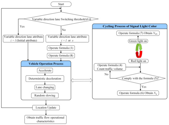
Figure 5.
Operation process chart of the proposed STCA-V model.
4. Numerical Simulation and Analysis
4.1. Classical Cellular Automaton Model
The theoretical research in the traffic field is mainly based on simulation experience, first proposed by Cremer and Ludwig in 1986 [51]. One is the CA model proposed by Neumann in the late 1940s [52]. In the field of mobility, it is considered a classical simulation model for studying microscopic traffic flows, i.e., the use of a large number of simple elements that run continuously through space-time using connections and arithmetic rules to simulate complex and polytropic phenomena.
The Spatio-temporal characteristics of traffic flows and the presence of random elements have led to many applications of the model in the field of transportation. In 1992, Nagel and Schreckenberg proposed the famous NaSch model (i.e., NS model) [24,53].
The NS model is discretized in time and space, distributing vehicles in a one-dimensional chain of discrete cells. Each cell has only two states, ‘0’ and ‘1’. Vn(t), Xn(t), and gapn(t) are used to denote the velocity, position, and spacing of the n th vehicle at moment t. The velocity V takes the values [0, Vmax]. Concerning the randomness of vehicle operation, a random slowing probability p is introduced. The NS model uses the following rules to update the state from t to t+1 for each vehicle, as shown in Equations (19)–(22):
As the basis for the cellular automaton model of traffic flow, the NS model relies on four simple operating rules for numerical simulation to reflect most traffic phenomena. However, the NS can only simulate the basic characteristics of viatic traffic flow, and cannot well represent the complex interrelationships in the traffic flow when the number of lanes increases and the road widens [54]. The single lane assumption and the no-overtaking assumption of the NS model constrain its further development. In 1997, Chowdhury proposed the first STCA model based on the NS model by introducing vehicle lane-changing rules [55]. The model was developed to satisfy the ‘two-lane rule’ in a traditional environment with realistic traffic conditions and has been gradually applied and improved by researchers. The STCA model describes vehicle lane changes using the following rules, shown in Equation (23):
In the above rules, gapn(t), gapn,other(t) and gapn,back(t) represent the distance between the n th vehicle and the vehicle ahead, the distance between the n th vehicle and the vehicle ahead in the adjacent lane, and the distance between the n th vehicle and the vehicle behind in the adjacent lane, respectively, at moment t. gapsafe is the limited safe distance in the model. The first term of Equation (5) shows that the n th vehicle is obstructed in the original lane. The second term of the above equation shows that the obstructed vehicle can find better conditions in the other lane. The third term of the above equation shows that if the lane is changed, the distance to the vehicle behind meets the safety conditions.
4.2. Simulation Environment Setting
As I-VICS is not yet widespread, the analyzed area of this study is limited to a three-lane road connecting to an intersection with a variable direction. The intersection is located at the end of the road, and there is no interference from vehicles coming from other directions. To validate the proposed model, MATLAB 2021a was chosen as the experimental platform for the numerical simulation of the STCA and STCA-V models. It is worth noting that the assumptions adopted in the simulation for the conditions of I-VICS are the same as the operating environment assumptions in Section 3.1.
Meanwhile, the simulated data were initialized according to the actual vehicle operating characteristics as follows:
- The vehicle model is based on micro and small vehicles with 9 seats or less.
- The types of driving vehicles were classified from fast to slow according to the driving speed.
- According to the speed limited values of urban roads, the speed of the classified driving vehicles was assigned a corresponding value.
The starting point of the discrete mesh was regarded as the departure point. The vehicle density ρ = n/L, where n is the number of vehicles in the road with a simulated lane length Lroad. According to the setting density speed [56], the initial vehicles were randomly distributed on the road from 0 to Vmax. To reduce the influence caused by the initial distribution, the simulation duration was 1000 steps, and the data was counted in the 500th to 1000th steps. The values and descriptions of the simulation parameters are shown in Table 1.

Table 1.
Traffic simulation parameters for cellular automaton.
4.3. Traffic Flow Parameters
In this paper, vehicles were identified using the variable direction lane switching factor threshold to determine the attributes of the variable direction lane. To ensure a balance between left-turn and straight traffic, vehicles switched lanes frequently to maintain or obtain better driving conditions. This is also reflected in the flow and the speed of the traffic. At the same time, the vehicles within the research environment were controlled by a signal. Hence, the phenomenon of stop and start waves also occurred on the corresponding road sections.
In the numerical simulation, the average speed and the flow rate of the STCA and the STCA-V models with different random slowing probabilities (Prd = 0.2, 0.3, 0.4) under different densities are analyzed. Figure 6 and Figure 7 show the corresponding basic graphs of average speed and flow, respectively.
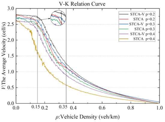
Figure 6.
Basic speed curve.
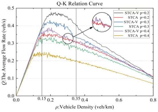
Figure 7.
Basic flow curve.
- 1
- Vehicle speed and flow are inversely proportional to the random slowing probability. Under the same random slowing probability, the velocities and the flow rates of both models show some variability, and the difference becomes more obvious as the density increases, especially when 0.15 veh/km < ρ < 0.35 veh/km, the difference is the largest. When ρ > 0.35 veh/km, the velocity and flow rate with the same random slowing probability gradually converge to synchronization.
- 2
- When ρ < 0.l5 veh/km, the speed and the flow rate of the STCA model are slightly lower than that of the STCA-V model. The reason is that the lane-changing requirements of the vehicles become greater with the increase of traffic density, and the STCA-V model can provide vehicles with the information ahead of the current road section in the I-VICS, and achieve safer and faster lane-changing through speed guidance to ensure the balanced and orderly operation of traffic flow.
- 3
- When 0.15 veh/km < ρ < 0.35 veh/km, the difference in vehicle speeds and flow rates simulated by the two models is the largest, i.e., the STCA-V model yields the greatest benefit. Moreover, both the speed and the flow curve output from the simulation show certain oscillations. The reason is that as the vehicle density increases, the queuing vehicles follow reduced waiting times and higher driving speeds for vehicle acceleration and deceleration with increasing lane-changing behavior. The mutual interference between the vehicles makes the average vehicle speed show an unstable oscillating downward trend.
- 4
- When ρ > 0.35 veh/km, the average speeds and the flows of both models tend to be synchronized. This is mainly because the higher traffic density and limited road capacity make more vehicle starts and stops and make it difficult for the vehicle to change lanes. Therefore, the vehicles cannot maintain optimal speed, leading to the failure of the lane-changing control method and weakening the benefits generated by the STCA-V model.
4.4. Analysis of Spatial and Temporal Characteristics
To analyze the Spatio-temporal characteristics, the vehicle density of 0.228 veh/km with a large difference in average flow is selected, and the random slowing probability is taken to be 0.2. Then the Spatio-temporal diagrams are plotted for the left-turn (L1) and variable direction lane (L2) and straight ahead (L3) for the two models, as shown in Figure 8. Figure 8a–c show the Spatio-temporal diagrams of lanes L1, L2, and L3 for the STCA model, respectively. Figure 8d–f show the Spatio-temporal diagrams of lanes L1, L2, and L3 for the STCA-V model. In this paper, the space-time diagram consists of data axes with horizontal coordinates representing the vehicle locations, vertical coordinates representing the time, black dots representing the vehicles, and white dots representing the empty cells.
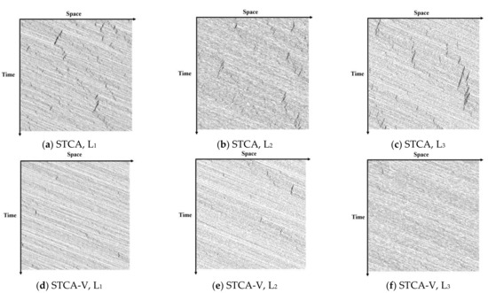
Figure 8.
Spatio-temporal characteristics of different CA models.
As can be seen from Figure 8:
- 1
- The number of dots in the STCA-V model is significantly less than that in the STCA model. This is because the STCA model is a passive lane-changing, and it is difficult for the vehicles to obtain the required safe lane-changing conditions under high density, resulting in frequent vehicle start-stop phenomenon manifested by the blocking phase appearing more frequently and lasting longer. In the STCA-V model, the success rate of vehicle lane-changing is improved, and the Spatio-temporal dot separation phenomenon is significantly improved because the vehicles can obtain lane attribute characteristics in advance and perform the active lane-changing operation according to the instruction.
- 2
- The STCA-V model results in a more balanced distribution of traffic between multiple lanes. This is due to the lack of lane-changing guidance and switching thresholds in the STCA model. Hence, the variable direction lanes cannot share the traffic volume in time, and the resulting deceleration, start-stop, and traffic flow turning imbalance is significant, reflected in the figure as the three lanes have a large number of dots that dissipate slowly. While in the STCA-V model, when the blocking phase in L1 occurs more frequently than L3, the functional switching threshold of L2 and the lane-changing guidance are activated. Thus, the vehicles have predictability in the driving process and equalize the traffic flow between the lanes to a certain extent. This improves the utilization of the variable direction lanes and shows that the blocking states of L1 and L2 tend to be the same while the free flow state of L3 is relatively more. According to the simulation output, the lane utilization increases by 6.84% and 22.8% when the corresponding attributes of L2 are straight ahead and left turn, respectively.
- 3
- This proves that the proposed STCA-V model works correctly according to the set rules. Also, the model is practically valid under ideal conditions and has some feasibility. Under the condition of vehicle infrastructure cooperative information interaction, the effective guidance on lane-changing behavior in the variable direction lane environment can change the way vehicles operate, alleviate the pressure of passing, and improve the level of control and efficiency of road use.
5. Conclusions
- Based on the premise that the information interaction between RSU and OBU of the vehicle-infrastructure cooperative system is guaranteed, the current problems in setting up the variable direction lanes and the operation process of the variable direction lanes after using the I-VICS system were analyzed.
- The light-color cycling strategy is proposed to simulate the phenomenon of traffic flow at intersections in gathering and dissipating waves, and mathematically describe the vehicle queuing and dissipating phenomena based on a cellular automaton model. As for the premise of combining the inter-vehicle information interaction and the real-time congestion state of the road, the induced vehicle speed and the variable direction lane thresholds were introduced and a cellular automaton operation rule was proposed that simulated the traffic operation characteristics of variable direction lanes in the I-VICS environment.
- The simulation analysis reveals that the proposed STCA-V model can better balance the flow imbalance phenomenon and improve both the average velocity and the average flow of the variable direction lane, with a maximum improvement of about 7.79% and 23.14% compared to the STCA model, respectively. Meanwhile, the model can reduce the frequency of blocking phases. The lane utilization increases by 6.84% and 22.8% when the variable direction lane attributes are straight ahead and left turn, respectively. It shows that the proposed STCA-V model can better adapt to the variable direction lane control mode in the I-VICS environment and provides a certain theoretical basis for constructing intelligent traffic development.
- In the future, our work will be conducted in the following terms:
- Since the subject and the research environment of this paper are in an ideal environment, there is a lack of change to the communication rules and there are gaps regarding more complex real traffic environments. At the same time, the I-VICS technology is not yet widely used and lacks actual measurement data. Therefore, the main direction for future research would be to consider combining the operation rules with the passage protocol for simulation experiments and visualizing the vehicle operation for intuitive analysis.
- As the development of I-VICS accelerates, the phase of mixed traffic flow will emerge. Therefore, in the case of mixed traffic flow with communication and non-communication vehicles, its effect on the operation of variable direction lanes can also be used in upcoming research.
Author Contributions
Conceptualization, Z.S. and F.S.; methodology, Z.S.; software, Z.S.; formal analysis, Z.S. and F.S.; investigation, Z.S. and Y.D.; resources, F.S. and G.Z.; data curation, R.Z.; writing—original draft preparation, Z.S.; writing—review and editing, F.S. and G.Z.; visualization, Z.S. and R.Z.; supervision, F.S.; project administration, F.S.; funding acquisition, F.S. and G.Z. All authors have read and agreed to the published version of the manuscript.
Funding
The Project was supported by the Foundation for Jiangsu Key Laboratory of Traffic and Transportation Security. (No. TTS2020-05) and the Science and Technology Planning Project of the Zibo City (Grant No. 2019ZBXC515).
Institutional Review Board Statement
Not applicable.
Informed Consent Statement
Not applicable.
Data Availability Statement
The data are not publicly available due to privacy restrictions.
Conflicts of Interest
The authors declare no conflict of interest.
References
- Jiang, T. Research on Variable Lane Setting Method of Signal Control Plane Intersection. Master’s Thesis, Chang’an University, Xi’an, China, 2019. [Google Scholar]
- Sun, F.; Wang, X.-L.; Zhang, Y.; Liu, W.-X.; Zhang, R.-J. Analysis of Bus Trip Characteristic Analysis and Demand Forecasting Based on GA-NARX Neural Network Model. IEEE Access 2020, 8, 8812–8820. [Google Scholar] [CrossRef]
- Sun, F.; Sun, L.; Ma, D.; Wang, Y.; Yao, R.; Zeng, Z. Optimal location of the U-turn at a signalised intersection with double left-turn lanes. IET Intell. Transp. Syst. 2018, 13, 531–540. [Google Scholar] [CrossRef]
- Ji-sheng, Z.; Bin, L.I.; Xiao-jing, W.; Fan, Z.; Xiao-liang, S.U.N. Design of Architecture and Development Roadmap of Smart Expressway. J. Highw. Transp. Res. Dev. 2018, 35, 88–94. [Google Scholar]
- Chen, X.; Li, Z.; Yang, Y.; Qi, L.; Ke, R. High-Resolution Vehicle Trajectory Extraction and Denoising from Aerial Videos. IEEE Trans. Intell. Transp. Syst. 2020, 22, 3190–3202. [Google Scholar] [CrossRef]
- Han, J.; Zhang, J.; Wang, X.; Liu, Y.; Wang, Q.; Zhong, F. An Extended Car-Following Model Considering Generalized Preceding Vehicles in V2X Environment. Futur. Internet 2020, 12, 216. [Google Scholar] [CrossRef]
- Fagnant, D.J.; Kockelman, K. Preparing a nation for autonomous vehicles: Opportunities, barriers and policy recommendations. Transp. Res. Part A Policy Pract. 2015, 77, 167–181. [Google Scholar] [CrossRef]
- Knorr, F.; Schreckenberg, M. Influence of inter-vehicle communication on peak hour traffic flow. Phys. A Stat. Mech. Appl. 2012, 391, 2225–2231. [Google Scholar] [CrossRef]
- Ye, L.; Yamamoto, T. Evaluating the impact of connected and autonomous vehicles on traffic safety. Phys. A Stat. Mech. Appl. 2019, 526, 121009. [Google Scholar] [CrossRef]
- Shi, Y. Optimization Control Schemes of UrbanTraffic Flow under Cooperative Vehicles Infrastructure Systems. Ph.D. Thesis, Shandong University, Shandong, China, 2017. [Google Scholar]
- Calvert, S.C.; Schakel, W.J.; van Lint, J.W.C. Will Automated Vehicles Negatively Impact Traffic Flow? J. Adv. Transp. 2017, 2017, 3082781. [Google Scholar] [CrossRef]
- Kerner, B.S. Failure of classical traffic flow theories: Stochastic highway capacity and automatic driving. Phys. A Stat. Mech. Appl. 2016, 450, 700–747. [Google Scholar] [CrossRef] [Green Version]
- Zhang, J.S.; Li, B.; Wang, X.J.; Zhang, F.; Sun, X.L. Smart Expressway Architecture and Development Path Design. Highw. Transp. Sci. Technol. 2018, 35, 88–94. [Google Scholar]
- Guo, G.; Xu, Y.; Xu, T.; Li, D.D.; Wang, Y.P.; Yuan, W. A Survey of Connected Shared Vehicle-Road Cooperative Intelligent Transportation Systems. Control Decis. 2019, 34, 2375–2389. [Google Scholar]
- Chang, X.; Li, H.; Qin, L.; Rong, J.; Lu, Y.; Chen, X. Evaluation of cooperative systems on driver behavior in heavy fog condition based on a driving simulator. Accid. Anal. Prev. 2019, 128, 197–205. [Google Scholar] [CrossRef] [PubMed]
- Shadrin, S.S.; Ivanova, A.A. Analytical review of standard SAE J3016 taxonomy and definitions for terms related to driving automation systems for on-road motor vehicles with latest updates. Avtomob. Doroga Infrastrukt. 2019, 3, 10. [Google Scholar]
- Hu, D.; Feng, X.; Zhao, X.; Li, H.; Ma, J.; Fu, Q. Impact of HMI on driver’s distraction on a freeway under heavy foggy condition based on visual characteristics. J. Transp. Saf. Secur. 2020, 1–24. [Google Scholar] [CrossRef]
- Zhang, Y.; Yao, D. Architecture for Intelligent Transportation Systems Based on Intelligent Vehicle-Infrastructure Cooperation Systems; Publishing House of Electronics Industry: Beijing, China, 2015. [Google Scholar]
- Liu, H.; Zhang, Y.; Zhang, K. Evaluating impacts of intelligent transit priority on intersection energy and emissions. Transp. Res. Part D Transp. Environ. 2020, 86, 102416. [Google Scholar] [CrossRef]
- Ding, J.; Xu, H.; Hu, J.; Zhang, Y. Centralized cooperative intersection control under automated vehicle environment. In Proceedings of the 2017 IEEE Intelligent Vehicles Symposium (IV), Redondo Beach, CA, USA, 11–14 June 2017; pp. 972–977. [Google Scholar]
- Treiber, M.; Hennecke, A.; Helbing, D. Congested traffic states in empirical observations and microscopic simulations. Phys. Rev. E 2000, 62, 1805–1824. [Google Scholar] [CrossRef] [PubMed] [Green Version]
- Li, Z.-P.; Liu, Y.-C. Analysis of stability and density waves of traffic flow model in an ITS environment. Eur. Phys. J. B 2006, 53, 367–374. [Google Scholar] [CrossRef]
- Zhang, H.M.; Jin, W.-L. Kinematic Wave Traffic Flow Model for Mixed Traffic. Transp. Res. Rec. 2002, 1802, 197–204. [Google Scholar] [CrossRef]
- Nagel, K.; Schreckenberg, M. A cellular automaton model for freeway traffic. J. Phys. I 1992, 2, 2221–2229. [Google Scholar] [CrossRef]
- Knospe, W.; Santen, L.; Schadschneider, A.; Schreckenberg, M. A realistic two-lane traffic model for highway traffic. J. Phys. A Math. Gen. 2002, 35, 3369–3388. [Google Scholar] [CrossRef]
- Knospe, W.; Santen, L.; Schadschneider, A.; Schreckenberg, M. Towards a realistic microscopic description of highway traffic. J. Phys. A Math. Gen. 2000, 33, L477–L485. [Google Scholar] [CrossRef]
- Jiang, R.; Wu, Q.-S. Cellular automata models for synchronized traffic flow. J. Phys. A Math. Gen. 2002, 36, 381–390. [Google Scholar] [CrossRef]
- Wang, Y. Study of Traffic Congestion’s Simulation Based on Cellular Automaton Model. J. Syst. Simul. 2010, 22, 2149–2154. [Google Scholar] [CrossRef]
- Li, X.-G.; Jia, B.; Gao, Z.-Y.; Jiang, R. A realistic two-lane cellular automata traffic model considering aggressive lane-changing behavior of fast vehicle. Phys. A Stat. Mech. Appl. 2006, 367, 479–486. [Google Scholar] [CrossRef]
- Jia, B.; Jiang, R.; Wu, Q.-S.; Hu, M.-B. Honk effect in the two-lane cellular automaton model for traffic flow. Phys. A Stat. Mech. Appl. 2005, 348, 544–552. [Google Scholar] [CrossRef]
- Shang, H.; Peng, Y. A new cellular automaton model for traffic flow considering realistic turn signal effect. Sci. China Ser. E Technol. Sci. 2012, 55, 1624–1630. [Google Scholar] [CrossRef]
- Xiang, Z.-T.; Gao, Z.; Zhang, T.; Che, K.; Chen, Y.-F. An improved two-lane cellular automaton traffic model based on BL-STCA model considering the dynamic lane-changing probability. Soft Comput. 2019, 23, 9397–9412. [Google Scholar] [CrossRef]
- Tian, J.; Li, G.; Treiber, M.; Jiang, R.; Jia, N.; Ma, S. Cellular automaton model simulating spatiotemporal patterns, phase transitions and concave growth pattern of oscillations in traffic flow. Transp. Res. Part B Methodol. 2016, 93, 560–575. [Google Scholar] [CrossRef]
- Li, X.; Qu, S.; Xia, Y. Cooperative Lane-Changing Rules on Multilane under Condition of Cooperative Vehicle and Infrastructure System. China J. Highw. Transp. 2014, 27, 97–104. [Google Scholar] [CrossRef]
- Young, K.L.; Salmon, P.M.; Lenné, M.G. At the cross-roads: An on-road examination of driving errors at intersections. Accid. Anal. Prev. 2013, 58, 226–234. [Google Scholar] [CrossRef]
- Ng, S.T.; Cheu, R.L.; Lee, D.-H. Simulation Evaluation of the Benefits of Real-Time Traffic Information to Trucks during Incidents. J. Intell. Transp. Syst. 2006, 10, 89–99. [Google Scholar] [CrossRef]
- Singh, S. Critical Reasons for Crashes Investigated in the National Motor Vehicle Crash Causation Survey. In Traffic Safety Facts; US Department of Transportation: Washington, DC, USA, 2015. [Google Scholar]
- Chen, M.; Tian, Y.; Fortino, G.; Zhang, J.; Humar, I. Cognitive Internet of Vehicles. Comput. Commun. 2018, 120, 58–70. [Google Scholar] [CrossRef]
- Treat, J.R.; Tumbas, N.S.; McDonald, S.T.; Shinar, D.; Hume, R.D.; Mayer, R.E.; Stansifer, R.L.; Castellan, N.J. Tri-Level Study of the Causes of Traffic Accidents: Final Report. Volume I: Casual Factor Tabulations and Assessments; Institute for Research in Public Safety: Bloomington, IN, USA, 1977. [Google Scholar] [CrossRef]
- Wang, Z. The Research on Combinatorial Optimization of Intersection Control Method Based on Variable Approach Lane and Signal Timing Optimization. Master’s Thesis, Southwest Jiaotong University, Sichuan, China, 2018. [Google Scholar]
- Cardaliaguet, P.; Forcadel, N. From Heterogeneous Microscopic Traffic Flow Models to Macroscopic Models. SIAM J. Math. Anal. 2021, 53, 309–322. [Google Scholar] [CrossRef]
- Zadobrischi, E.; Cosovanu, L.-M.; Dimian, M. Traffic Flow Density Model and Dynamic Traffic Congestion Model Simulation Based on Practice Case with Vehicle Network and System Traffic Intelligent Communication. Symmetry 2020, 12, 1172. [Google Scholar] [CrossRef]
- Chen, X.; Chen, H.; Yang, Y.; Wu, H.; Zhang, W.; Zhao, J.; Xiong, Y. Traffic Flow Prediction by an Ensemble Framework with Data Denoising and Deep Learning Model. Phys. Stat. Mech. Appl. 2021, 565, 125574. [Google Scholar] [CrossRef]
- Jing, M.; Deng, W.; Wang, H.; Ji, Y.-J. Two-Lane Cellular Automaton Traffic Model Based on Car Following Behavior. Acta Phys. Sin. 2012, 61, 244502. [Google Scholar] [CrossRef]
- China Society of Automotive Engineers. Cooperative Intelligent Transportation System; Vehicular Communication. Application Layer Specification and Data Exchange Standard: T/CSAE 53-2017. 2017. Available online: http://csae.sae-china.org/b29.html (accessed on 9 December 2021).
- Li, X.; Ma, W.; Zhao, Z.; Zhang, K.; Wang, X. Improved STCA Lane Changing Model for Two-Lane Road Based on Driving Guidance under CVIS. J. Southeast Univ. Nat. Sci. Ed. 2020, 50, 1134–1142. [Google Scholar] [CrossRef]
- Li, X.; Zhao, Z. An Improved NS Model for Single Lane with Induce Speed under Situation of Cooperative Vehicle Infrastructure System. J. Highw. Transp. Res. Dev. 2018, 35, 101–108. [Google Scholar] [CrossRef]
- Jia, N.; Ma, S.-F.; Zhong, S.-Q. Analytical investigation of the boundary-triggered phase transition dynamics in a cellular automata model with a slow-to-start rule. Chin. Phys. B 2012, 21, 42–47. [Google Scholar] [CrossRef]
- Barlovic, R.; Huisinga, T.; Schadschneider, A.; Schreckenberg, M. Open boundaries in a cellular automaton model for traffic flow with metastable states. Phys. Rev. E 2002, 66, 046113. [Google Scholar] [CrossRef] [PubMed]
- Li, D. Research on Left-Turn Variable Lane of Signalized Intersections Based on Queue Length. Master’s Thesis, Southwest Jiaotong University, Sichuan, China, 2017. [Google Scholar]
- Cremer, M.; Ludwig, J. A fast simulation model for traffic flow on the basis of boolean operations. Math. Comput. Simul. 1986, 28, 297–303. [Google Scholar] [CrossRef]
- Neumann, J.; Burks, A.W. Theory of Self-Reproducing Automata; University of Illinois Press Urbana: Champaign-Urbana, IL, USA, 1966; Volume 1102024. [Google Scholar]
- Jia, B.; Gao, Z.-Y.; Li, K.; Li, X.-G. Models and Simulations of Traffic System Based on the Theory of Cellular Automaton. Sci. Beijing 2007, 123, 2002. [Google Scholar]
- Lv, W.; Song, W.-G.; Liu, X.-D.; Ma, J. A microscopic lane changing process model for multilane traffic. Phys. A Stat. Mech. Its Appl. 2013, 392, 1142–1152. [Google Scholar] [CrossRef]
- Chowdhury, D.; Wolf, D.E.; Schreckenberg, M. Particle hopping models for two-lane traffic with two kinds of vehicles: Effects of lane-changing rules. Phys. A Stat. Mech. Appl. 1997, 235, 417–439. [Google Scholar] [CrossRef]
- Code for Design of Urban Road Engineering; Ministry of Housing and Urban-Rural Development of the People’s Republic of China: Beijing, China, 2012.
Publisher’s Note: MDPI stays neutral with regard to jurisdictional claims in published maps and institutional affiliations. |
© 2021 by the authors. Licensee MDPI, Basel, Switzerland. This article is an open access article distributed under the terms and conditions of the Creative Commons Attribution (CC BY) license (https://creativecommons.org/licenses/by/4.0/).