
Short-Term Unit Commitment by Using Machine Learning to Cover the Uncertainty of Wind Power Forecasting


Abstract
:1. Introduction
2. Research Contributions
- This research may help the electricity supply companies to minimize the operational costs and to have a reliable plan for short-term planning strategies.
- Ensure the stability in the network, since a sufficient number of units will be committed to meet the demand and will help to cut down overall losses or fuel costs by employing the most cost-effective unit; hence, the demand can be provided by that unit functioning at its optimum efficiency.
3. Techniques to Solve the UC Problem
3.1. Deterministic Techniques
3.2. Metaheuristic Techniques
3.3. Hybrid Techniques
4. Identification of the UC Problem
4.1. Objective Function
4.2. Constraints
4.2.1. Power Balance
4.2.2. Power Bounds
4.2.3. Ramping Limits
4.2.4. Minimum ON and OFF Time
4.2.5. Operating Reserve
4.2.6. Spinning Reserve
4.3. Power Losses
5. Wind Forecasting Using a Recurrent Neural Network
5.1. Uncertainty of Renewable Energy Sources
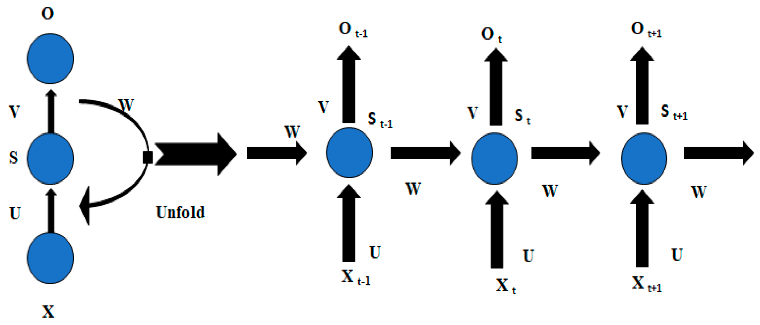
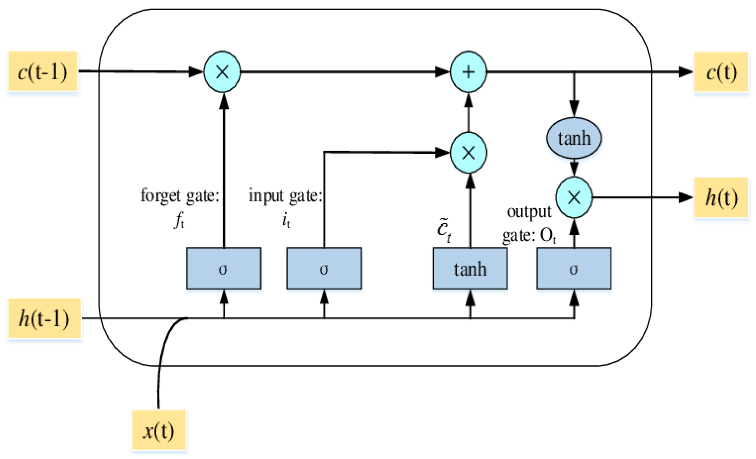
5.2. Recurrent Neural Network
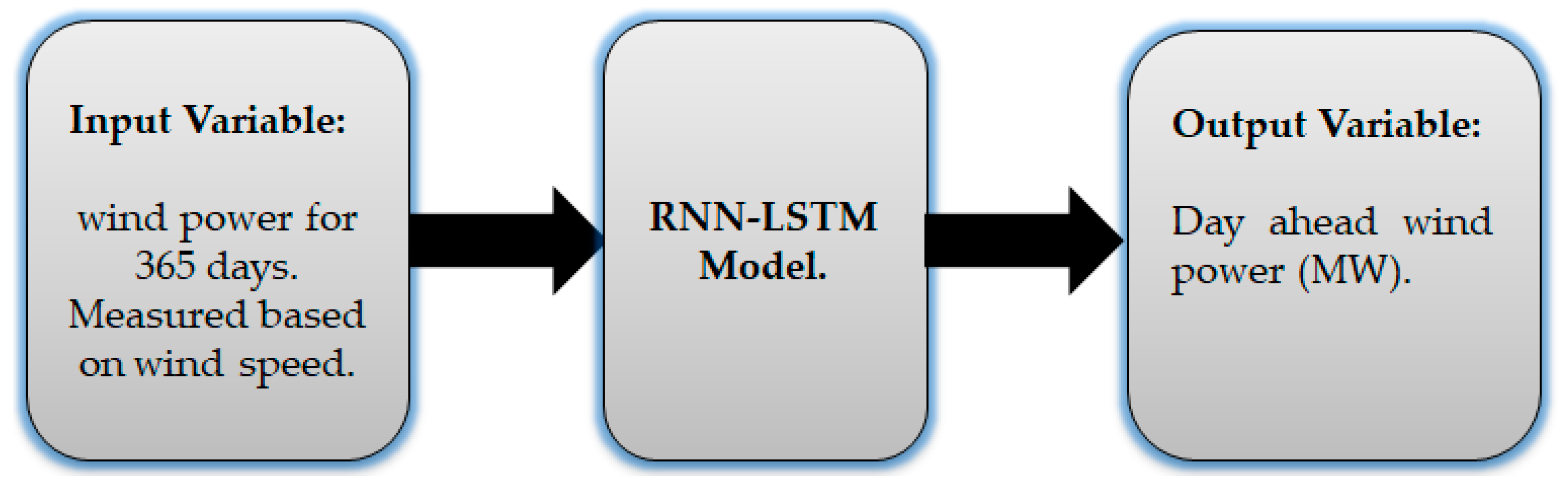
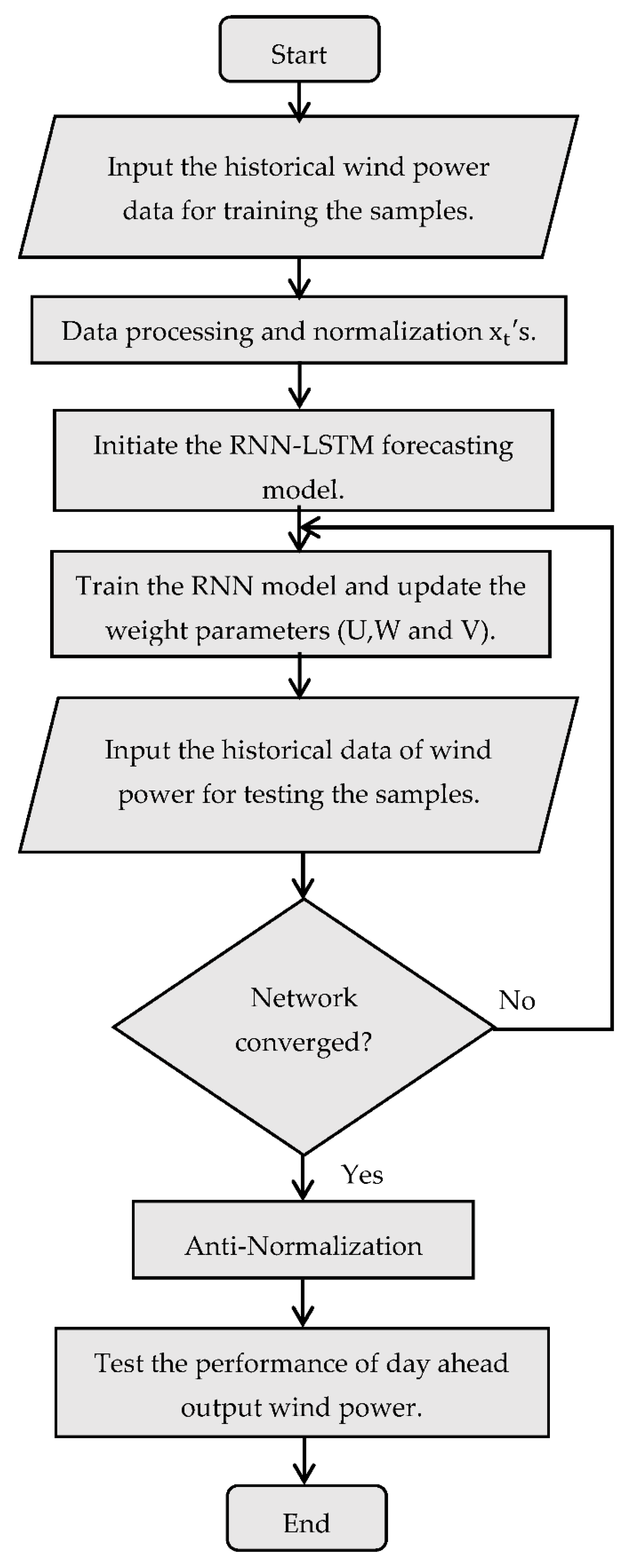
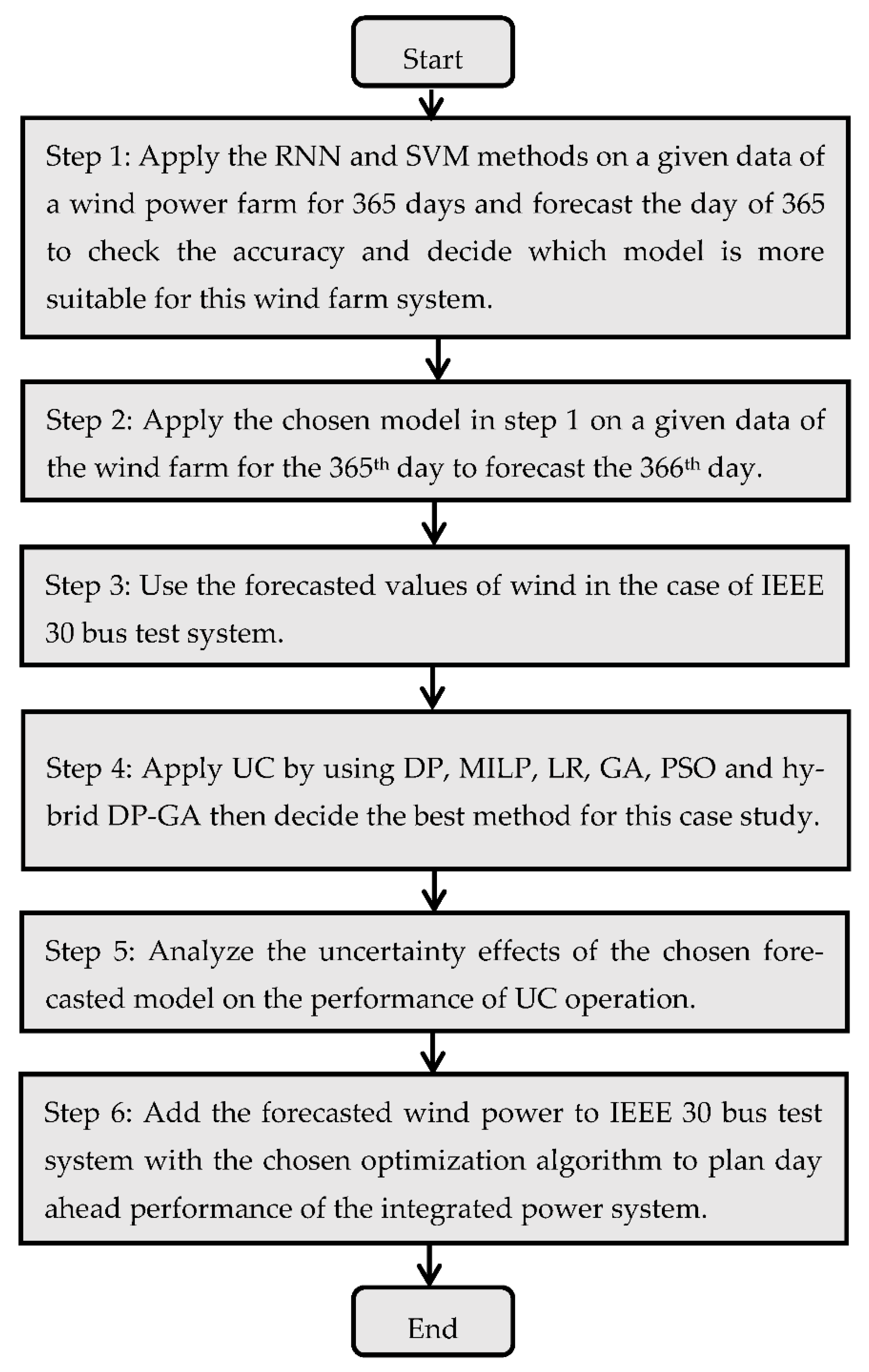
6. Methodology
7. Case Study
8. Results and Discussions
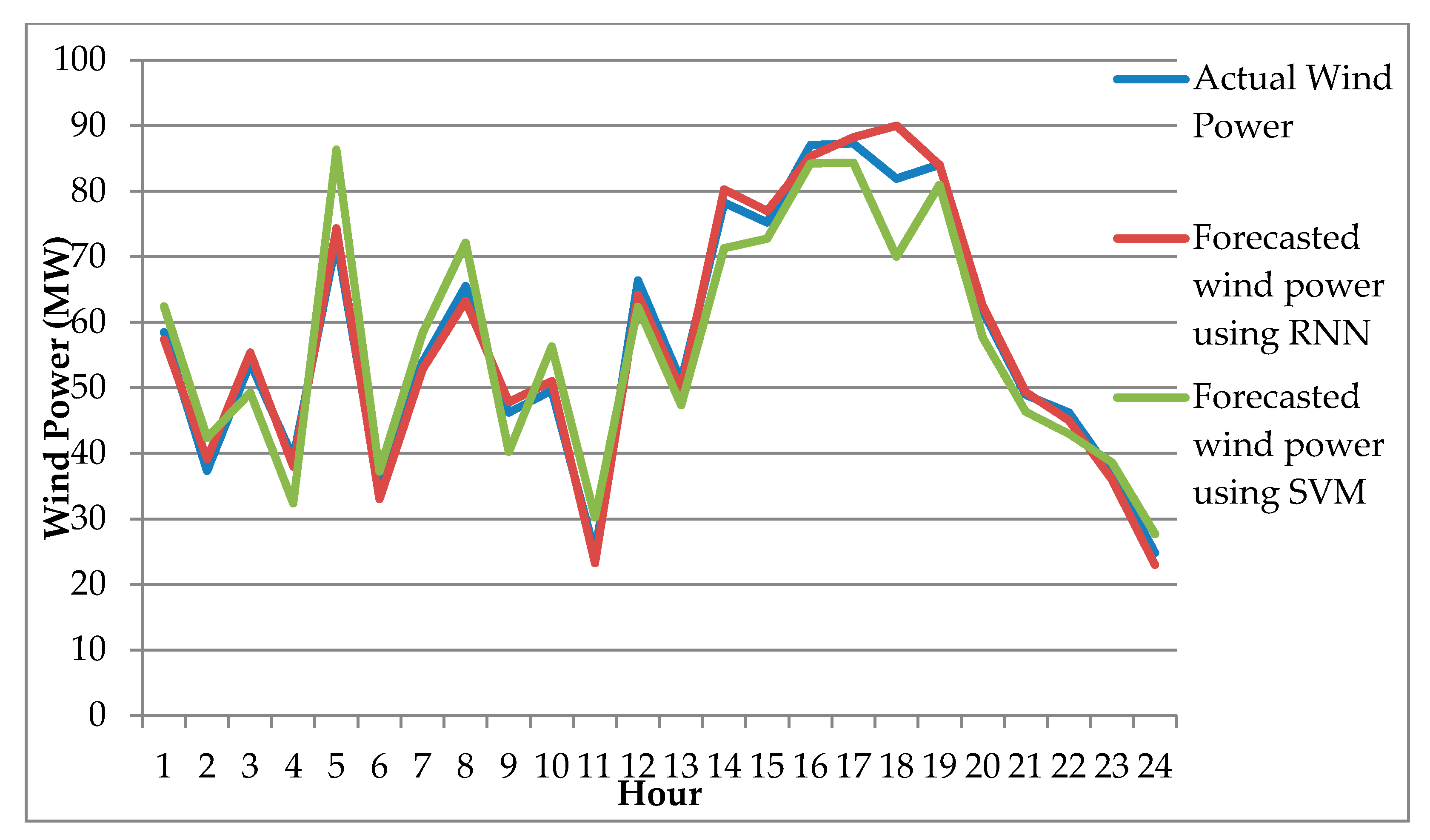
8.1. Testing the Proposed Forecasting Methodology
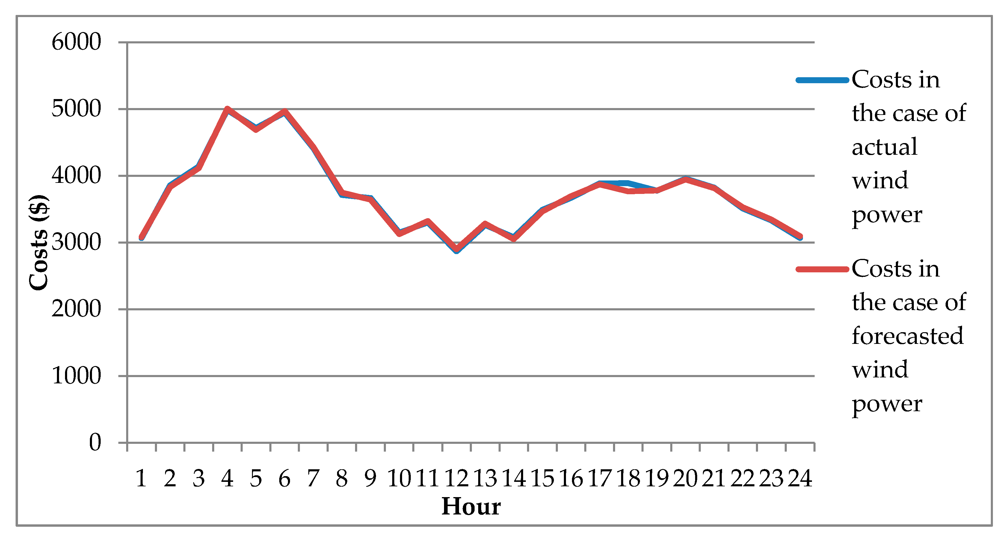
8.2. RNN Uncertainty Effects
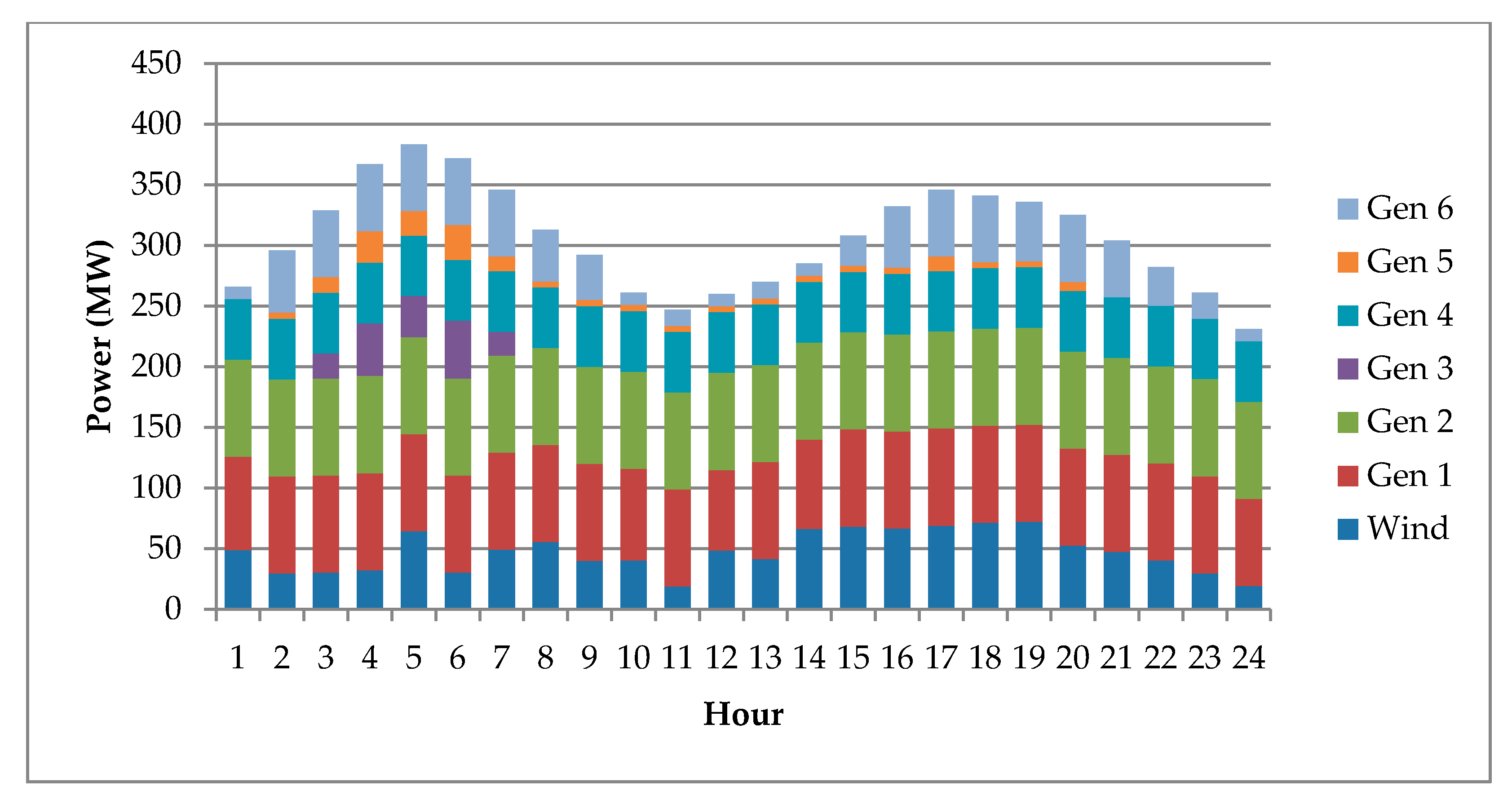
8.3. Day-Ahead UC Planning
9. Conclusions
Author Contributions
Funding
Conflicts of Interest
Nomenclatures
| Symbol/Abbreviation | Meaning |
| CNN | Convolution neural networks |
| DP | Dynamic programming |
| ED | Economic dispatch |
| GA | Genetic algorithm |
| LR | Lagrangian relaxation |
| LSTM | Long short Term memory |
| MILP | Mixed integer linear programming |
| PSO | Particle swarm optimization |
| RNN | Rcurrent neural network |
| SVM | Support vector machine |
| UC | Unit commitment |
| Pit | Power generation of unit i at time t |
| Iit | Commitment state of unit i at time t |
| SUit | Start-up cost of unit i at time t |
| SDit | Shut-down cost of unit i at time t |
| αi, βi and γi | Generator i cost coefficients |
| PW,it | Wind power of unit i at time t |
| PD,t | The system demand at time t |
| PL,t | The system losses at time t |
| Pi,min | Minimum power generation of unit i |
| Pi,max | Maximum power generation of unit i |
| URi | Ramp-up rate of unit i |
| DRi | Ramp-down rate of unit i |
| RO,t | Operating reserve at time t |
| Rs,t | Spinning reserve at time t |
| xt | RNN input value at time t |
| st | RNN hidden layeres at time t |
| ot | RNN output value at time t |
| U, W, V | Weight values |
| I | Input gate |
| F | Forget gate |
| O | Output gate |
| g | Candidate or hidden state |
References
- Ma, Z.; Zhong, H.; Xia, Q.; Kang, C.; Wang, Q.; Cao, X. A unit commitment algorithm with relaxation-based neighborhood search and improved relaxation inducement. IEEE Trans. Power Syst. 2020, 35, 3800–3809. [Google Scholar] [CrossRef]
- Yang, Y.; Wu, W.; Wang, B.; Li, M. Analytical solution for stochastic unit commitment considering wind power uncertainty with gaussian mixture model. IEEE Trans. Power Syst. 2019, 35, 2769–2782. [Google Scholar] [CrossRef]
- Gaddam, R.R. Optimal Unit Commitment Using Swarm Intelligence for Secure Operation of Solar Energy Integrated Smart Grid; Power Systems Research Center; International Institute of Information Technology: Hyderabad, India, 2013. [Google Scholar]
- Mehranpour, A.; Ramezani, M. Unit commitment in the presence of photovoltaic cells. In Proceedings of the 1st Conference on Applied Research in Electrical Engineering (AREE), Ahvaz, Iran, 27 January 2020; Volume 2020, pp. 1–9. [Google Scholar]
- Abdou, I.; Tkiouat, M. Unit commitment problem in electrical power system: A literature review. Int. J. Electr. Comput. Eng. 2018, 8, 1357–1372. [Google Scholar] [CrossRef]
- Abdi, H. Profit-based unit commitment problem: A review of models, methods, challenges, and future directions total revenue. Renew. Sustain. Energy Rev. 2021, 138, 110504. [Google Scholar] [CrossRef]
- Vargas, D.V.; Murata, J.; Takano, H. Tackling unit commitment and load dispatch problems considering all constraints with evolutionary computation. arXiv 2019, arXiv:1903.09304. [Google Scholar]
- Furukakoi, M.; Adewuyi, O.B.; Matayoshi, H.; Howlader, A.M.; Senjyu, T. Multi objective unit commitment with voltage stability and PV uncertainty. Appl. Energy. 2018, 228, 618–623. [Google Scholar] [CrossRef]
- Wang, C.; Li, X.; Wang, Z.; Dong, X.; Liang, Z.; Liu, X.; Liang, J.; Han, X. Day-ahead unit commitment method considering time sequence feature of wind power forecast error. Int. J. Electr. Power Energy Syst. 2018, 98, 156–166. [Google Scholar] [CrossRef]
- Shabbir, N.; Kutt, L.; Jawad, M.; Amadiahanger, R.; Iqbal, M.N.; Rosin, A. Wind Energy Forecasting Using Recurrent Neural Networks. In Proceedings of the 2019 Big Data, Knowledge and Control Systems Engineering (BdKCSE), Sofia, Bulgaria, 21–22 November 2019; pp. 1–5. [Google Scholar]
- Thakur, N.; Titare, L.S. Determination of unit commitment problem using dynamic programming. Int. J. Nov. Res. Electr. Mech. Eng. 2016, 3, 24–28. [Google Scholar]
- Arora, V.; Chanana, S. Solution to unit commitment problem using Lagrangian relaxation and Mendel’s GA method. In Proceedings of the 2016 International Conference on Emerging Trends in Electrical Electronics & Sustainable Energy Systems (ICETEESES), Sultanpur, India, 11–12 March 2016; Volume 2016, pp. 126–129. [Google Scholar]
- Alvarez, G.E.; Marcovecchio, M.G.; Aguirre, P. Security constrained unit commitment scheduling: A new MILP formulation for solving transmission constraints. Comput. Chem. Eng. 2018, 115, 455–473. [Google Scholar] [CrossRef]
- Hu, G.; Yang, L. The parallel interior point for solving the continuous optimization problem of unit commitment. In Proceedings of the 2016 9th International Congress on Image and Signal Processing, BioMedical Engineering and Informatics (CISP-BMEI), Datong, China, 15–17 October 2016; pp. 1333–1338. [Google Scholar]
- Palis, D.; Palis, S. Efficient unit commitment—A modified branch-and-bound approach. In Proceedings of the 2016 IEEE Region 10 Conference (TENCON), Singapore, 22–25 November 2016; Volume 2017, pp. 267–271. [Google Scholar]
- McLarty, D.; Panossian, N.; Jabbari, F.; Traverso, A. Dynamic economic dispatch using complementary quadratic pro-gramming. Energy 2019, 166, 755–764. [Google Scholar] [CrossRef]
- Madraswala, H.S. Modified genetic algorithm solution to unit commitment problem. In Proceedings of the 2017 International Conference on Nascent Technologies in Engineering (ICNTE), Navi Mumbai, India, 27–28 January 2017; pp. 1–6. [Google Scholar]
- Logenthiran, T.; Srinivasan, D. Particle swarm optimization for unit commitment problem. In Proceedings of the 2010 IEEE 11th International Conference on Probabilistic Methods Applied to Power Systems, Singapore, 14–17 June 2010; Volume 2010, pp. 642–647. [Google Scholar]
- Reddy, S.; Kumar, R.; Panigrahi, B.K. Binary bat search algorithm for unit commitment problem in power system. In Proceedings of the 2017 IEEE International WIE Conference on Electrical and Computer Engineering (WIECON-ECE), Dehradun, Indi, 18–19 December 2018; pp. 121–124. [Google Scholar]
- Majidi, H.; Emadaleslami, M.; Haghifam, M.R. A new binary-coded approach to the unit commitment problem using grey wolf optimization. In Proceedings of the 2020 28th Iranian Conference on Electrical Engineering (ICEE), Tabriz, Iran, 4–6 August 2020; pp. 1–5. [Google Scholar]
- Kokare, M.B.; Tade, S.V. Application of Artificial Bee Colony Method for Unit Commitment. In Proceedings of the 2018 4th International Conference on Computing Communication Control and Automation (ICCUBEA), Pune, India, 16–18 August 2018; pp. 1–6. [Google Scholar]
- Rouhi, F.; Effatnejad, R. Unit commitment in power system t by combination of dynamic programming (DP), genetic algorithm (GA) and particle swarm optimization (PSO). Indian J. Sci. Technol. 2015, 8, 134–141. [Google Scholar] [CrossRef]
- Boqtob, O.; El Moussaoui, H.; El Markhi, H.; Lamhamdi, T. Optimal robust unit commitment of microgrid using hybrid particle swarm optimization with sine cosine acceleration coefficients. Int. J. Renew. Energy Res. 2019, 9, 1125–1134. [Google Scholar]
- Kamboj, V.K. A novel hybrid PSO–GWO approach for unit commitment problem. Neural Comput. Appl. 2016, 27, 1643–1655. [Google Scholar] [CrossRef]
- Singh, A.; Khamparia, A. A hybrid whale optimization-differential evolution and genetic algorithm based approach to solve unit commitment scheduling problem: WODEGA. Sustain. Comput. Inform. Syst. 2020, 28, 100442. [Google Scholar] [CrossRef]
- Wang, J.; Shahidehpour, M.; Li, Z. Security-constrained unit commitment with volatile wind power generation. IEEE Trans. Power Syst. 2008, 23, 1319–1327. [Google Scholar] [CrossRef]
- Huang, W.T.; Yao, K.C.; Chen, M.K.; Wang, F.Y.; Zhu, C.H.; Chang, Y.R.; Lee, Y.D.; Ho, Y.H. Derivation and application of a new transmission loss formula for power system economic dispatch. Energies 2018, 11, 417. [Google Scholar] [CrossRef] [Green Version]
- Wulandhari, L.A.; Komsiyah, S.; Wicaksono, W. Bat algorithm implementation on economic dispatch optimization problem. Procedia Comput. Sci. 2018, 135, 275–282. [Google Scholar] [CrossRef]
- Liu, M.; Quilumba, F.; Lee, W.-J. Dispatch scheduling for a wind farm with hybrid energy storage based on wind and LMP forecasting. IEEE Trans. Ind. Appl. 2015, 51, 1970–1977. [Google Scholar] [CrossRef]
- Mohy-Ud-Din, G.; Vu, D.H.; Muttaqi, K.M.; Sutanto, D. An integrated energy management approach for the economic operation of industrial microgrids under uncertainty of renewable energy. IEEE Trans. Ind. Appl. 2020, 56, 1062–1073. [Google Scholar] [CrossRef] [Green Version]
- Alqunun, K. Optimal Unit commitment problem considering stochastic wind energy penetration. Eng. Technol. Appl. Sci. Res. 2020, 10, 6316–6322. [Google Scholar] [CrossRef]
- Zhang, Y.; Liu, Y.; Shu, S.; Zheng, F.; Huang, Z. A data-driven distributionally robust optimization model for multi-energy coupled system considering the temporal-spatial correlation and distribution uncertainty of renewable energy sources. Energy 2021, 216, 119171. [Google Scholar] [CrossRef]
- Zhu, Y.; Liu, X.; Deng, R.; Zhai, Y. Memetic algorithm for solving monthly unit commitment problem considering uncertain wind power. J. Control Autom. Electr. Syst. 2020, 31, 511–520. [Google Scholar] [CrossRef]
- Ming, B.; Liu, P.; Guo, S.; Cheng, L.; Zhou, Y.; Gao, S.; Li, H. Robust hydroelectric unit commitment considering integration of large-scale photovoltaic power: A case study in China. Appl. Energy 2018, 228, 1341–1352. [Google Scholar] [CrossRef]
- Ning, C.; You, F. Data-driven adaptive robust unit commitment under wind power uncertainty: A Bayesian nonparametric approach. IEEE Trans. Power Syst. 2019, 34, 2409–2418. [Google Scholar] [CrossRef]
- Rachunok, B.; Staid, A.; Watson, J.P.; Woodruff, D.L.; Yang, D. Stochastic unit commitment performance considering monte carlo wind power scenarios. In Proceedings of the 2018 IEEE International Conference on Probabilistic Methods Applied to Power Systems (PMAPS), Boise, ID, USA, 24–28 June 2018; pp. 1–6. [Google Scholar]
- Sivaneasan, B.; Yu, C.Y.; Goh, K.P. Solar forecasting using ANN with fuzzy logic pre-processing. Energy Procedia 2017, 143, 727–732. [Google Scholar] [CrossRef]
- Bedi, J.; Toshniwal, D. Deep learning framework to forecast electricity demand. Appl. Energy 2019, 238, 1312–1326. [Google Scholar] [CrossRef]
- Wang, H.; Lei, Z.; Zhang, X.; Zhou, B.; Peng, J. A review of deep learning for renewable energy forecasting. Energy Convers. Manag. 2019, 198, 111799. [Google Scholar] [CrossRef]
- Abd Al-Azeem Hussieny, O.; El-Beltagy, M.A.; El-Tantawy, S. Forecasting of renewable energy using ANN, GPANN and ANFIS (A comparative study and performance analysis). In Proceedings of the 2nd Novel Intelligent Leading Emerging Sciences Conference (NILES), Giza, Egypt, 24–26 October 2020; pp. 54–59. [Google Scholar]
- Dong, D.; Sheng, Z.; Yang, T. Wind power prediction based on recurrent neural network with long short-term memory units. In Proceedings of the 2018 International Conference on Renewable Energy and Power Engineering (REPE), Toronto, ON, Canada, 24–26 November 2018; Volume 2019, pp. 34–38. [Google Scholar]
- Blanchard, T.; Samanta, B. Wind speed forecasting using neural networks. Wind Eng. 2020, 44, 33–48. [Google Scholar] [CrossRef]
- Pang, Z.; Niu, F.; O’Neill, Z. Solar radiation prediction using recurrent neural network and artificial neural network: A case study with comparisons. Renew. Energy 2020, 156, 279–289. [Google Scholar] [CrossRef]
- Li, L.L.; Zhao, X.; Tseng, M.L.; Tan, R.R. Short-term wind power forecasting based on support vector machine with improved dragonfly algorithm. J. Clean. Prod. 2020, 242, 118447. [Google Scholar] [CrossRef]
- Abbas, Z.; Al-Shishtawy, A.; Girdzijauskas, S.; Vlassov, V. Short-term traffic prediction using long short-term memory neural networks. In Proceedings of the 2018 IEEE International Congress on Big Data (BigData Congress), Seattle, WA, USA, 10–13 December 2018; Volume 1, pp. 57–65. [Google Scholar]
- Liu, C.; Jin, Z.; Gu, J.; Qiu, C. Short-term load forecasting using a long short-term memory network. In Proceedings of the 2017 IEEE PES Innovative Smart Grid Technologies Conference Europe (ISGT-Europe), Torino, Italy, 26–29 September 2017; Volume 2018, pp. 1–6. [Google Scholar]
- Kamh, M.; Abdelaziz, A.Y.; Mekhamer, S.F.; Badr, M.A. Modified augmented hopfield neural network for optimal thermal unit commitment. In Proceedings of the 2009 IEEE Power & Energy Society General Meeting, Calgary, AB, Canada, 26–30 July 2009; pp. 1–8. [Google Scholar]
- Ananthan, D. Unit commitment solution using particle swarm optimisation (PSO). IOSR J. Eng. 2014, 4, 48–55. [Google Scholar] [CrossRef]
- Ding, Y. Wind Time Series Dataset; CRC Press: Boca Raton, FL, USA, 2021. [Google Scholar] [CrossRef]


| Unit | Bus | Pmin (MW) | Pmax (MW) | Min ON Time (h) | Min OFF Time (h) | Ramp up | Ramp down | Cost Coefficients | Start up Cost | Shut down Cost | ||
|---|---|---|---|---|---|---|---|---|---|---|---|---|
| α | β | γ | ||||||||||
| 1 | 1 | 15 | 80 | 2 | 2 | 50 | 75 | 0.02 | 15 | 0 | 350 | 0 |
| 2 | 2 | 15 | 80 | 2 | 2 | 80 | 100 | 0.0175 | 14.75 | 0 | 400 | 0 |
| 3 | 5 | 10 | 50 | 3 | 3 | 100 | 120 | 0.025 | 16 | 0 | 500 | 0 |
| 4 | 8 | 10 | 50 | 4 | 4 | 80 | 100 | 0.0625 | 14 | 0 | 60 | 0 |
| 5 | 11 | 5 | 30 | 3 | 3 | 50 | 75 | 0.025 | 16 | 0 | 60 | 0 |
| 6 | 23 | 10 | 55 | 4 | 4 | 80 | 100 | 0.0083 | 15.25 | 0 | 60 | 0 |
| Coefficient B | Value | Coefficient B | Value |
|---|---|---|---|
| B1 | 0.015751 | B24 | 0.036122 |
| B2 | 0.004148 | B25 | 0.021162 |
| B3 | −0.0163430 | B26 | 0.037327 |
| B4 | −0.0041543 | B33 | 0.035597 |
| B5 | −0.0070962 | B34 | 0.016785 |
| B6 | 0.008479 | B35 | 0.00187 |
| B11 | 0.026653 | B36 | 0.01678 |
| B12 | 0.032813 | B44 | 0.04962 |
| B13 | 0.007563 | B45 | 0.023143 |
| B14 | 0.017716 | B46 | 0.034977 |
| B15 | 0.003144 | B55 | 0.013355 |
| B16 | 0.020161 | B56 | 0.014568 |
| B22 | 0.054859 | B66 | 0.054766 |
| B23 | 0.02842 |
| Hour | Load Demand (MW) | Hour | Load Demand (MW) |
|---|---|---|---|
| 1 | 266 | 13 | 270 |
| 2 | 296 | 14 | 285 |
| 3 | 329 | 15 | 308 |
| 4 | 367 | 16 | 332 |
| 5 | 383.4 | 17 | 346 |
| 6 | 360 | 18 | 341 |
| 7 | 346 | 19 | 336 |
| 8 | 313 | 20 | 325 |
| 9 | 292 | 21 | 304 |
| 10 | 261 | 22 | 282 |
| 11 | 247 | 23 | 261 |
| 12 | 260 | 24 | 231 |
| Hour | Wind Power (MW) Day 1 | ... | Hour | Wind Power (MW) Day 365 |
|---|---|---|---|---|
| 1 | 38.02373 | ... | 1 | 58.48118 |
| 2 | 30.17464 | ... | 2 | 37.32334 |
| 3 | 29.60595 | ... | 3 | 53.79952 |
| 4 | 12.38366 | ... | 4 | 39.27922 |
| 5 | 14.70253 | ... | 5 | 72.55551 |
| 6 | 15.39127 | ... | 6 | 34.4053 |
| 7 | 23.17681 | ... | 7 | 53.91672 |
| 8 | 19.25512 | ... | 8 | 65.53804 |
| 9 | 19.96631 | ... | 9 | 46.22368 |
| 10 | 21.33149 | ... | 10 | 49.59142 |
| 11 | 11.75611 | ... | 11 | 24.69124 |
| 12 | 2.375202 | ... | 12 | 66.39924 |
| 13 | 1.96187 | ... | 13 | 50.94851 |
| 14 | 4.324661 | ... | 14 | 78.26047 |
| 15 | 5.510049 | ... | 15 | 75.25145 |
| 16 | 6.874369 | ... | 16 | 87.02105 |
| 17 | 11.74694 | ... | 17 | 87.29366 |
| 18 | 9.093303 | ... | 18 | 81.91527 |
| 19 | 12.53907 | ... | 19 | 84.05596 |
| 20 | 10.12221 | ... | 20 | 61.79108 |
| 21 | 19.45207 | ... | 21 | 48.95232 |
| 22 | 21.67068 | ... | 22 | 46.22508 |
| 23 | 32.18356 | ... | 23 | 36.92015 |
| 24 | 32.34231 | ... | 24 | 24.83013 |
| Actual Wind Power (MW) | Forecasted Wind Power (MW) | |||
|---|---|---|---|---|
| RNN | Error (%) | SVM | Error (%) | |
| 58.48118 | 57.356 | 1.924 | 62.423 | 3.94182 |
| 37.32334 | 39.123 | 3.152 | 42.365 | 5.04166 |
| 53.79952 | 55.356 | 2.89 | 49.254 | 4.54552 |
| 39.27922 | 37.985 | 3.294 | 32.365 | 6.91422 |
| 72.55551 | 74.325 | 2.438 | 86.352 | 13.79649 |
| 34.4053 | 33.0215 | 4.022 | 37.25 | 2.8447 |
| 53.91672 | 52.8796 | 1.923 | 58.365 | 4.44828 |
| 65.53804 | 63.2586 | 3.478 | 72.1452 | 6.60716 |
| 46.22368 | 47.8 | 3.4102 | 40.254 | 5.96968 |
| 49.59142 | 51.0258 | 2.892 | 56.324 | 6.73258 |
| 24.69124 | 23.2574 | 1.43384 | 30.214 | 5.52276 |
| 66.39924 | 64.2158 | 3.288 | 62.352 | 4.04724 |
| 50.94851 | 49.6869 | 2.476 | 47.3652 | 3.58331 |
| 78.26047 | 80.2548 | 2.548 | 71.3256 | 6.93487 |
| 75.25145 | 76.9582 | 2.268 | 72.785 | 2.46645 |
| 87.02105 | 85.3365 | 1.935 | 84.236 | 2.78505 |
| 87.29366 | 88.2358 | 1.079 | 84.365 | 2.92866 |
| 81.91527 | 90.02587 | 9.901 | 70.0175 | 11.89777 |
| 84.05596 | 83.9785 | 0.092 | 80.985 | 3.07096 |
| 61.79108 | 62.5148 | 1.171 | 57.6859 | 4.10518 |
| 48.95232 | 49.325 | 0.761 | 46.358 | 2.59432 |
| 46.22508 | 45.0025 | 2.644 | 42.9857 | 3.23938 |
| 36.92015 | 36.0258 | 2.422 | 41.6231 | 3.70295 |
| 24.83013 | 22.958 | 1.87213 | 27.691 | 2.86087 |
| Average error (%) | 2.638% | 5.025% | ||
| Hour | Day-Ahead Forecasted Wind Power (MW) | Hour | Day-Ahead Forecasted Wind Power (MW) |
|---|---|---|---|
| 1 | 48.6582 | 13 | 41.325 |
| 2 | 29.6584 | 14 | 66.254 |
| 3 | 30.2569 | 15 | 68.2368 |
| 4 | 32.2584 | 16 | 66.5981 |
| 5 | 64.2658 | 17 | 68.9862 |
| 6 | 30.3695 | 18 | 71.2586 |
| 7 | 49.2563 | 19 | 72.02586 |
| 8 | 55.36985 | 20 | 52.3697 |
| 9 | 39.9985 | 21 | 47.2562 |
| 10 | 40.2584 | 22 | 40.3691 |
| 11 | 18.6985 | 23 | 29.6859 |
| 12 | 48.3694 | 24 | 19.0258 |
| Hour | DP | MILP | LR | GA | PSO | DP-GA |
|---|---|---|---|---|---|---|
| 1 | 3264 | 3388 | 3234 | 3217 | 3219 | 3212 |
| 2 | 3985 | 4087 | 4140 | 3985 | 3975 | 3978 |
| 3 | 4506 | 4648 | 4579 | 4526 | 4521 | 4515 |
| 4 | 5156 | 5208 | 5213 | 5100 | 5092 | 5096 |
| 5 | 4858 | 4872 | 4885 | 4858 | 4838 | 4847 |
| 6 | 5284 | 5346 | 5335 | 5303 | 5314 | 5011 |
| 7 | 4480 | 4541 | 4571 | 4497 | 4490 | 4488 |
| 8 | 3875 | 3927 | 3947 | 3872 | 3882 | 3867 |
| 9 | 3787 | 3817 | 3802 | 3822 | 3755 | 3761 |
| 10 | 3295 | 3329 | 3330 | 3297 | 3292 | 3289 |
| 11 | 3399 | 3418 | 3423 | 3380 | 3390 | 3391 |
| 12 | 3152 | 3210 | 3212 | 3145 | 3151 | 3138 |
| 13 | 3411 | 3439 | 3435 | 3423 | 3416 | 3410 |
| 14 | 3258 | 3339 | 3306 | 3258 | 3266 | 3260 |
| 15 | 3633 | 3655 | 3633 | 3644 | 3591 | 3597 |
| 16 | 3986 | 4076 | 3987 | 4003 | 3972 | 3980 |
| 17 | 4173 | 4314 | 4213 | 4214 | 4186 | 4172 |
| 18 | 4071 | 4211 | 4044 | 4044 | 4045 | 4054 |
| 19 | 4010 | 4079 | 4006 | 3975 | 3966 | 3961 |
| 20 | 4161 | 4183 | 4165 | 4086 | 4131 | 4104 |
| 21 | 3836 | 3879 | 3906 | 3843 | 3837 | 3847 |
| 22 | 3633 | 3558 | 3626 | 3635 | 3619 | 3599 |
| 23 | 3433 | 3520 | 3460 | 3427 | 3444 | 3440 |
| 24 | 3144 | 3283 | 3201 | 3150 | 3163 | 3154 |
| Total cost | 93,790 | 95,327 | 94,653 | 93,704 | 93,555 | 93,171 |
| Hour | Load (MW) | Units Commitment | Output Power (MW) | Cost ($) | ||||||||||||
|---|---|---|---|---|---|---|---|---|---|---|---|---|---|---|---|---|
| W | G1 | G2 | G3 | G4 | G5 | G6 | W | G1 | G2 | G3 | G4 | G5 | G6 | |||
| 1 | 266 | 1 | 1 | 1 | 0 | 1 | 0 | 1 | 58.481 | 68.8 | 80 | 0 | 50 | 0 | 10 | 3064.9 |
| 2 | 296 | 1 | 1 | 1 | 0 | 1 | 0 | 1 | 37.3233 | 80 | 80 | 0 | 50 | 0 | 51 | 3857.7 |
| 3 | 329 | 1 | 1 | 1 | 0 | 1 | 1 | 1 | 53.7995 | 80 | 80 | 0 | 50 | 13.7 | 55 | 4138.4 |
| 4 | 367 | 1 | 1 | 1 | 1 | 1 | 1 | 1 | 39.2792 | 80 | 80 | 41.6 | 50 | 24.9 | 55 | 4983.6 |
| 5 | 383.4 | 1 | 1 | 1 | 1 | 1 | 1 | 1 | 72.5555 | 80 | 80 | 31.1 | 50 | 18.6 | 55 | 4714.8 |
| 6 | 360 | 1 | 1 | 1 | 1 | 1 | 1 | 1 | 34.4053 | 80 | 80 | 40.2 | 50 | 24 | 55 | 4946.8 |
| 7 | 346 | 1 | 1 | 1 | 1 | 1 | 1 | 1 | 53.9167 | 80 | 80 | 19.1 | 50 | 11.8 | 55 | 4413 |
| 8 | 313 | 1 | 1 | 1 | 0 | 1 | 1 | 1 | 65.538 | 80 | 80 | 0 | 50 | 5 | 36.2 | 3711.9 |
| 9 | 292 | 1 | 1 | 1 | 0 | 1 | 1 | 1 | 46.2237 | 80 | 80 | 0 | 50 | 5 | 33.2 | 3666.4 |
| 10 | 261 | 1 | 1 | 1 | 0 | 1 | 1 | 1 | 49.5914 | 69.1 | 80 | 0 | 50 | 5 | 10 | 3148.5 |
| 11 | 247 | 1 | 1 | 1 | 0 | 1 | 1 | 1 | 24.6912 | 79.1 | 80 | 0 | 50 | 5 | 10 | 3299.7 |
| 12 | 260 | 1 | 1 | 1 | 0 | 1 | 1 | 1 | 66.3992 | 50.3 | 80 | 0 | 50 | 5 | 10 | 2867.5 |
| 13 | 270 | 1 | 1 | 1 | 0 | 1 | 1 | 1 | 50.9485 | 76.7 | 80 | 0 | 50 | 5 | 10 | 3263.8 |
| 14 | 285 | 1 | 1 | 1 | 0 | 1 | 1 | 1 | 78.2605 | 64.5 | 80 | 0 | 50 | 5 | 10 | 3080 |
| 15 | 308 | 1 | 1 | 1 | 0 | 1 | 1 | 1 | 75.2515 | 80 | 80 | 0 | 50 | 5 | 21.6 | 3490.1 |
| 16 | 332 | 1 | 1 | 1 | 0 | 1 | 1 | 1 | 87.0211 | 80 | 80 | 0 | 50 | 5 | 33.3 | 3668.6 |
| 17 | 346 | 1 | 1 | 1 | 0 | 1 | 1 | 1 | 87.2937 | 80 | 80 | 0 | 50 | 5 | 47.5 | 3884.4 |
| 18 | 341 | 1 | 1 | 1 | 0 | 1 | 1 | 1 | 81.9153 | 80 | 80 | 0 | 50 | 5 | 47.8 | 3888.8 |
| 19 | 336 | 1 | 1 | 1 | 0 | 1 | 1 | 1 | 84.056 | 80 | 80 | 0 | 50 | 5 | 40.5 | 3777.3 |
| 20 | 325 | 1 | 1 | 1 | 0 | 1 | 1 | 1 | 61.7911 | 80 | 80 | 0 | 50 | 5 | 52.2 | 3955.8 |
| 21 | 304 | 1 | 1 | 1 | 0 | 1 | 0 | 1 | 48.9523 | 80 | 80 | 0 | 50 | 0 | 48.6 | 3820.9 |
| 22 | 282 | 1 | 1 | 1 | 0 | 1 | 0 | 1 | 46.2251 | 80 | 80 | 0 | 50 | 0 | 28.1 | 3509.2 |
| 23 | 261 | 1 | 1 | 1 | 0 | 1 | 0 | 1 | 36.9202 | 80 | 80 | 0 | 50 | 0 | 16.3 | 3329.2 |
| 24 | 231 | 1 | 1 | 1 | 0 | 1 | 0 | 1 | 24.8301 | 69 | 80 | 0 | 50 | 0 | 10 | 3066.9 |
| Total Costs ($) | 89,548.2 | |||||||||||||||
| Hour | Load (MW) | Units Commitment | Output Power (MW) | Cost ($) | ||||||||||||
|---|---|---|---|---|---|---|---|---|---|---|---|---|---|---|---|---|
| W | G1 | G2 | G3 | G4 | G5 | G6 | W | G1 | G2 | G3 | G4 | G5 | G6 | |||
| 1 | 266 | 1 | 1 | 1 | 0 | 1 | 0 | 1 | 57.356 | 69.9 | 80 | 0 | 50 | 0 | 10 | 3081.8 |
| 2 | 296 | 1 | 1 | 1 | 0 | 1 | 0 | 1 | 39.123 | 80 | 80 | 0 | 50 | 0 | 49.2 | 3830.3 |
| 3 | 329 | 1 | 1 | 1 | 1 | 1 | 0 | 1 | 55.356 | 80 | 80 | 12.2 | 50 | 0 | 55 | 4113.5 |
| 4 | 367 | 1 | 1 | 1 | 1 | 1 | 1 | 1 | 37.985 | 80 | 80 | 42.4 | 50 | 25.4 | 55 | 5004.3 |
| 5 | 383.4 | 1 | 1 | 1 | 1 | 1 | 1 | 1 | 74.325 | 80 | 80 | 30 | 50 | 18 | 55 | 4686.5 |
| 6 | 360 | 1 | 1 | 1 | 1 | 1 | 1 | 1 | 33.0215 | 80 | 80 | 41.1 | 50 | 24.6 | 55 | 4969 |
| 7 | 346 | 1 | 1 | 1 | 1 | 1 | 1 | 1 | 52.8796 | 80 | 80 | 19.7 | 50 | 12.2 | 55 | 4429.6 |
| 8 | 313 | 1 | 1 | 1 | 0 | 1 | 1 | 1 | 63.2586 | 80 | 80 | 0 | 50 | 5 | 38.5 | 3746.7 |
| 9 | 292 | 1 | 1 | 1 | 0 | 1 | 1 | 1 | 47.8 | 80 | 80 | 0 | 50 | 5 | 31.6 | 3642.3 |
| 10 | 261 | 1 | 1 | 1 | 0 | 1 | 1 | 1 | 51.0258 | 67.6 | 80 | 0 | 50 | 5 | 10 | 3127 |
| 11 | 247 | 1 | 1 | 1 | 0 | 1 | 1 | 1 | 23.2574 | 80 | 80 | 0 | 50 | 5 | 10.6 | 3321.4 |
| 12 | 260 | 1 | 1 | 1 | 0 | 1 | 1 | 1 | 64.2158 | 52.5 | 80 | 0 | 50 | 5 | 10 | 2900.3 |
| 13 | 270 | 1 | 1 | 1 | 0 | 1 | 1 | 1 | 49.6869 | 78 | 80 | 0 | 50 | 5 | 10 | 3282.8 |
| 14 | 285 | 1 | 1 | 1 | 0 | 1 | 1 | 1 | 80.2548 | 62.5 | 80 | 0 | 50 | 5 | 10 | 3050.1 |
| 15 | 308 | 1 | 1 | 1 | 0 | 1 | 1 | 1 | 76.9582 | 80 | 80 | 0 | 50 | 5 | 19.9 | 3464.1 |
| 16 | 332 | 1 | 1 | 1 | 0 | 1 | 1 | 1 | 85.3365 | 80 | 80 | 0 | 50 | 5 | 35 | 3694.3 |
| 17 | 346 | 1 | 1 | 1 | 0 | 1 | 1 | 1 | 88.2358 | 80 | 80 | 0 | 50 | 5 | 46.5 | 3870 |
| 18 | 341 | 1 | 1 | 1 | 0 | 1 | 1 | 1 | 90.0259 | 80 | 80 | 0 | 50 | 5 | 39.7 | 3765.1 |
| 19 | 336 | 1 | 1 | 1 | 0 | 1 | 1 | 1 | 83.9785 | 80 | 80 | 0 | 50 | 5 | 40.5 | 3778.5 |
| 20 | 325 | 1 | 1 | 1 | 0 | 1 | 1 | 1 | 62.5148 | 80 | 80 | 0 | 50 | 5 | 51.4 | 3944.7 |
| 21 | 304 | 1 | 1 | 1 | 0 | 1 | 0 | 1 | 49.325 | 80 | 80 | 0 | 50 | 0 | 48.2 | 3815.2 |
| 22 | 282 | 1 | 1 | 1 | 0 | 1 | 0 | 1 | 45.0025 | 80 | 80 | 0 | 50 | 0 | 29.4 | 3527.9 |
| 23 | 261 | 1 | 1 | 1 | 0 | 1 | 0 | 1 | 36.0258 | 80 | 80 | 0 | 50 | 0 | 17.2 | 3342.8 |
| 24 | 231 | 1 | 1 | 1 | 0 | 1 | 0 | 1 | 22.958 | 70.8 | 80 | 0 | 50 | 0 | 10 | 3095 |
| Total Costs ($) | 89,483.2 | |||||||||||||||
| Hour | Costs with Actual Wind Values ($) | Costs with Forecasted Wind Value ($) | Uncertainty (%) |
|---|---|---|---|
| 1 | 3064.9 | 3081.8 | 0.55 |
| 2 | 3857.7 | 3830.3 | 0.71 |
| 3 | 4138.4 | 4113.5 | 0.60 |
| 4 | 4983.6 | 5004.3 | 0.41 |
| 5 | 4714.8 | 4686.5 | 0.60 |
| 6 | 4946.8 | 4969 | 0.44 |
| 7 | 4413 | 4429.6 | 0.37 |
| 8 | 3711.9 | 3746.7 | 0.93 |
| 9 | 3666.4 | 3642.3 | 0.65 |
| 10 | 3148.5 | 3127 | 0.68 |
| 11 | 3299.7 | 3321.4 | 0.65 |
| 12 | 2867.5 | 2900.3 | 1.14 |
| 13 | 3263.8 | 3282.8 | 0.58 |
| 14 | 3080 | 3050.1 | 0.97 |
| 15 | 3490.1 | 3464.1 | 0.74 |
| 16 | 3668.6 | 3694.3 | 0.70 |
| 17 | 3884.4 | 3870 | 0.37 |
| 18 | 3888.8 | 3765.1 | 3.18 |
| 19 | 3777.3 | 3778.5 | 0.031 |
| 20 | 3955.8 | 3944.7 | 0.28 |
| 21 | 3820.9 | 3815.2 | 0.15 |
| 22 | 3509.2 | 3527.9 | 0.53 |
| 23 | 3329.2 | 3342.8 | 0.40 |
| 24 | 3066.9 | 3095 | 0.91 |
| Total Cost | 89,548.2 | 89,483.2 | 0.0725 |
| Hour | Load (MW) | PL,t (MW) | Units Commitment | Output Power (MW) | Cost ($) | ||||||||||||
|---|---|---|---|---|---|---|---|---|---|---|---|---|---|---|---|---|---|
| Wind | G1 | G2 | G3 | G4 | G5 | G6 | Wind | G1 | G2 | G3 | G4 | G5 | G6 | ||||
| 1 | 266 | 1.3 | 1 | 1 | 1 | 0 | 1 | 0 | 1 | 48.6582 | 78.6 | 80 | 0 | 50 | 0 | 10 | 3212 |
| 2 | 296 | 2.315 | 1 | 1 | 1 | 0 | 1 | 1 | 1 | 29.6584 | 80 | 80 | 0 | 50 | 5 | 53.7 | 3978 |
| 3 | 329 | 3.52 | 1 | 1 | 1 | 1 | 1 | 1 | 1 | 30.2569 | 80 | 80 | 23.0 | 50 | 14.2 | 55 | 4515 |
| 4 | 367 | 3.82 | 1 | 1 | 1 | 1 | 1 | 1 | 1 | 32.2584 | 80 | 80 | 45.9 | 50 | 27.6 | 55 | 5096 |
| 5 | 383.4 | 3.9 | 1 | 1 | 1 | 1 | 1 | 1 | 1 | 64.2658 | 80 | 80 | 36 | 50 | 21.6 | 55 | 4847 |
| 6 | 360 | 3.65 | 1 | 1 | 1 | 1 | 1 | 1 | 1 | 30.3695 | 80 | 80 | 42.7 | 50 | 25.6 | 55 | 5011 |
| 7 | 346 | 3.8 | 1 | 1 | 1 | 1 | 1 | 1 | 1 | 49.2563 | 80 | 80 | 21.9 | 50 | 13.6 | 55 | 4488 |
| 8 | 313 | 3.72 | 1 | 1 | 1 | 0 | 1 | 1 | 1 | 55.36985 | 80 | 80 | 0 | 50 | 5 | 46.4 | 3867 |
| 9 | 292 | 2.42 | 1 | 1 | 1 | 0 | 1 | 1 | 1 | 39.9985 | 80 | 80 | 0 | 50 | 5 | 39.4 | 3761 |
| 10 | 261 | 2.65 | 1 | 1 | 1 | 0 | 1 | 1 | 1 | 40.2584 | 78.4 | 80 | 0 | 50 | 5 | 10 | 3289 |
| 11 | 247 | 1.83 | 1 | 1 | 1 | 0 | 1 | 1 | 1 | 18.6985 | 80 | 80 | 0 | 50 | 5 | 15.1 | 3391 |
| 12 | 260 | 1.724 | 1 | 1 | 1 | 0 | 1 | 1 | 1 | 48.3694 | 68.4 | 80 | 0 | 50 | 5 | 10 | 3138 |
| 13 | 270 | 2.695 | 1 | 1 | 1 | 0 | 1 | 1 | 1 | 41.325 | 80 | 80 | 0 | 50 | 5 | 16.4 | 3410 |
| 14 | 285 | 2.75 | 1 | 1 | 1 | 0 | 1 | 1 | 1 | 66.254 | 76.5 | 80 | 0 | 50 | 5 | 10 | 3260 |
| 15 | 308 | 3.89 | 1 | 1 | 1 | 0 | 1 | 1 | 1 | 68.2368 | 80 | 80 | 0 | 50 | 5 | 28.7 | 3597 |
| 16 | 332 | 3.365 | 1 | 1 | 1 | 0 | 1 | 1 | 1 | 66.5981 | 80 | 80 | 0 | 50 | 5 | 53.8 | 3980 |
| 17 | 346 | 3.785 | 1 | 1 | 1 | 0 | 1 | 1 | 1 | 68.9862 | 80 | 80 | 0 | 50 | 15.8 | 55 | 4172 |
| 18 | 341 | 3.695 | 1 | 1 | 1 | 0 | 1 | 1 | 1 | 71.2586 | 80 | 80 | 0 | 50 | 8.4 | 55 | 4054 |
| 19 | 336 | 3.524 | 1 | 1 | 1 | 0 | 1 | 1 | 1 | 72.02586 | 80 | 80 | 0 | 50 | 5 | 52.5 | 3961 |
| 20 | 325 | 3.963 | 1 | 1 | 1 | 0 | 1 | 1 | 1 | 52.3697 | 80 | 80 | 0 | 50 | 11.6 | 55 | 4104 |
| 21 | 304 | 3.526 | 1 | 1 | 1 | 0 | 1 | 0 | 1 | 47.2562 | 80 | 80 | 0 | 50 | 0 | 50.3 | 3847 |
| 22 | 282 | 2.365 | 1 | 1 | 1 | 0 | 1 | 0 | 1 | 40.3691 | 80 | 80 | 0 | 50 | 0 | 34 | 3599 |
| 23 | 261 | 2.254 | 1 | 1 | 1 | 0 | 1 | 0 | 1 | 29.6859 | 80 | 80 | 0 | 50 | 0 | 23.6 | 3440 |
| 24 | 231 | 2.785 | 1 | 1 | 1 | 0 | 1 | 0 | 1 | 19.0258 | 74.8 | 80 | 0 | 50 | 0 | 10 | 3154 |
| Total Cost | 93,171 | ||||||||||||||||
Publisher’s Note: MDPI stays neutral with regard to jurisdictional claims in published maps and institutional affiliations. |
© 2021 by the authors. Licensee MDPI, Basel, Switzerland. This article is an open access article distributed under the terms and conditions of the Creative Commons Attribution (CC BY) license (https://creativecommons.org/licenses/by/4.0/).
Share and Cite
Salman, D.; Kusaf, M. Short-Term Unit Commitment by Using Machine Learning to Cover the Uncertainty of Wind Power Forecasting. Sustainability 2021, 13, 13609. https://doi.org/10.3390/su132413609
Salman D, Kusaf M. Short-Term Unit Commitment by Using Machine Learning to Cover the Uncertainty of Wind Power Forecasting. Sustainability. 2021; 13(24):13609. https://doi.org/10.3390/su132413609
Chicago/Turabian StyleSalman, Diaa, and Mehmet Kusaf. 2021. "Short-Term Unit Commitment by Using Machine Learning to Cover the Uncertainty of Wind Power Forecasting" Sustainability 13, no. 24: 13609. https://doi.org/10.3390/su132413609
APA StyleSalman, D., & Kusaf, M. (2021). Short-Term Unit Commitment by Using Machine Learning to Cover the Uncertainty of Wind Power Forecasting. Sustainability, 13(24), 13609. https://doi.org/10.3390/su132413609