Optimization of X-ray Tube Voltage to Improve the Precision of Two Phase Flow Meters Used in Petroleum Industry
Abstract
1. Introduction
2. Materials and Method
2.1. Detection System
2.2. X-ray Tube Voltage Optimization Procedure
3. Results and Discussion
4. Conclusions
Author Contributions
Funding
Institutional Review Board Statement
Informed Consent Statement
Data Availability Statement
Conflicts of Interest
References
- Almutairi, Z.; Al-Alweet, F.M.; Alghamdi, Y.A.; Almisned, O.A.; Alothman, O.Y. Investigating the characteristics of two-phase flow using electrical capacitance tomography (ECT) for three pipe orientations. Processes 2020, 8, 51. [Google Scholar] [CrossRef]
- Yang, Y.; Wang, D.; Niu, P.; Liu, M.; Wang, S. Gas-liquid two-phase flow measurements by the electromagnetic flowmeter combined with a phase-isolation method. Flow Meas. Instrum. 2018, 60, 78–87. [Google Scholar] [CrossRef]
- Wongsaroj, W.; Hamdani, A.; Thong-Un, N.; Takahashi, H.; Kikura, H. Extended short-time fourier transform for ultrasonic velocity profiler on two-phase bubbly flow using a single resonant frequency. Appl. Sci. 2019, 9, 50. [Google Scholar] [CrossRef]
- Roshani, G.H.; Nazemi, E.; Feghhi, S.A.H. Investigation of using 60Co source and one detector for determining the flow regime and void fraction in gas–liquid two-phase flows. Flow Meas. Instrum. 2016, 50, 73–79. [Google Scholar] [CrossRef]
- Roshani, M.; Phan, G.; Roshani, G.H.; Hanus, R.; Nazemi, B.; Corniani, E.; Nazemi, E. Combination of X-ray tube and GMDH neural network as a nondestructive and potential technique for measuring characteristics of gas-oil–water three phase flows. Measurement 2021, 168, 108427. [Google Scholar] [CrossRef]
- Asano, H.; Takenaka, N.; Fujii, T. Flow characteristics of gas–liquid two-phase flow in plate heat exchanger: (Visualization and void fraction measurement by neutron radiography). Exp. Therm. Fluid Sci. 2004, 28, 223–230. [Google Scholar] [CrossRef]
- Hewitt, G.F.; Roberts, D.N. Studies of Two-Phase Flow Patterns by Simultaneous X-Ray and Flast Photography; No. AERE-M-2159; Atomic Energy Research Establishment: Harwell, UK, 1969. [Google Scholar]
- Jones, O.C., Jr.; Zuber, N. The interrelation between void fraction fluctuations and flow patterns in two-phase flow. Int. J. Multiph. Flow 1975, 2, 273–306. [Google Scholar] [CrossRef]
- Harvel, G.D.; Hori, K.; Kawanishi, K.; Chang, J.S. Cross-sectional void fraction distribution measurements in a vertical annulus two-phase flow by high speed X-ray computed tomography and real-time neutron radiography techniques. Flow Meas. Instrum. 1999, 10, 259–266. [Google Scholar] [CrossRef]
- Fischer, F.; Hampel, U. Ultra fast electron beam X-ray computed tomography for two-phase flow measurement. Nucl. Eng. Des. 2010, 240, 2254–2259. [Google Scholar] [CrossRef]
- Song, K.; Liu, Y. A compact x-ray system for two-phase flow measurement. Meas. Sci. Technol. 2018, 29, 025305. [Google Scholar] [CrossRef]
- Roshani, M.; Ali, P.J.M.; Roshani, G.H.; Nazemi, B.; Corniani, E.; Phan, N.H.; Tran, H.N.; Nazemi, E. X-ray tube with artificial neural network model as a promising alternative for radioisotope source in radiation based two phase flowmeters. Appl. Radiat. Isot. 2020, 164, 109255. [Google Scholar] [CrossRef]
- Amiri, S.; Ali, P.J.M.; Mohammed, S.; Hanus, R.; Abdulkareem, L.; Alanezi, A.A.; Eftekhari-Zadeh, E.; Roshani, G.H.; Nazemi, E.; Kalmoun, E.M. Proposing a nondestructive and intelligent system for simultaneous determining flow regime and void fraction percentage of gas–liquid two phase flows using polychromatic X-ray transmission spectra. J. Nondestruct. Eval. 2021, 40, 1–12. [Google Scholar] [CrossRef]
- Mäkiharju, S.A.; Gabillet, C.; Paik, B.G.; Chang, N.A.; Perlin, M.; Ceccio, S.L. Time-resolved two-dimensional X-ray densitometry of a two-phase flow downstream of a ventilated cavity. Exp. Fluids 2013, 54, 1–21. [Google Scholar] [CrossRef]
- Tekawade, A.; Sforzo, B.A.; Matusik, K.E.; Fezzaa, K.; Kastengren, A.L.; Powell, C.F. Time-resolved 3D imaging of two-phase fluid flow inside a steel fuel injector using synchrotron X-ray tomography. Sci. Rep. 2020, 10, 1–9. [Google Scholar]
- Heindel, T.J. A review of X-ray flow visualization with applications to multiphase flows. J. Fluids Eng. 2011, 133, 074001. [Google Scholar] [CrossRef]
- Pelowitz, D.B. MCNP-X TM User’s Manual, Version 2.5.0. LA-CP-05e0369; Los Alamos National Laboratory: Los Alamos, NM, USA, 2005. [Google Scholar]
- Karami, A.; Roshani, G.H.; Khazaei, A.; Nazemi, E.; Fallahi, M. Investigation of different sources in order to optimize the nuclear metering system of gas-oil-water annular flows. Neural Comput. Appl. 2020, 32, 3619–3631. [Google Scholar] [CrossRef]
- Roshani, M.; Phan, G.T.; Ali, P.J.M.; Roshani, G.H.; Hanus, R.; Duong, T.; Corniani, E.; Nazemi, E.; Kalmoun, E.M. Evaluation of flow pattern recognition and void fraction measurement in two phase flow independent of oil pipeline’s scale layer thickness. Alex. Eng. J. 2021, 60, 1955–1966. [Google Scholar] [CrossRef]
- Salgado, C.M.; Pereira, C.M.; Schirru, R.; Brandão, L.E. Flow regime identification and volume fraction prediction in multiphase flows by means of gamma-ray attenuation and artificial neural networks. Prog. Nucl. Energy 2010, 52, 555–562. [Google Scholar] [CrossRef]
- Nazemi, E.; Feghhi, S.; Roshani, G.; Setayeshi, S.A.; Peyvandi, R.G. A radiation-based hydrocarbon two-phase flow meter for estimating of phase fraction independent of liquid phase density in stratified regime. Flow Meas. Instrum. 2015, 46, 25–32. [Google Scholar] [CrossRef]
- Nazemi, E.; Feghhi, S.; Roshani, G.; Peyvandi, R.G.; Setayeshi, S. Precise void fraction measurement in two-phase flows independent of the flow regime using gamma-ray attenuation. Nucl. Eng. Technol. 2016, 48, 64–71. [Google Scholar] [CrossRef]
- Roshani, G.; Nazemi, E.; Roshani, M. Identification of flow regime and estimation of volume fraction independent of liquid phase density in gas-liquid two-phase flow. Prog. Nucl. Energy 2017, 98, 29–37. [Google Scholar] [CrossRef]
- Roshani, G.H.; Nazemi, E.; Roshani, M.M. Flow regime independent volume fraction estimation in three-phase flows using dual-energy broad beam technique and artificial neural network. Neural Comput. Appl. 2016, 28, 1265–1274. [Google Scholar] [CrossRef]
- Buhmann, M.D. Radial Basis Functions: Theory and Implementations; Cambridge University: Cambridge, UK, 2003; ISBN 0-521-63338-9. [Google Scholar]
- Aleksandrov, A.N.; Kishchenko, M.A.; Van, T.N. Simulating the formation of wax deposits in wells using electric submersible pumps. In Advances in Raw Material Industries for Sustainable Development Goals; CRC Press: London, UK, 2021; pp. 283–295. [Google Scholar] [CrossRef]
- Khounani, Z.; Hosseinzadeh-Bandbafha, H.; Nazemi, F.; Shaeifi, M.; Karimi, K.; Tabatabaei, M.; Aghbashlo, M.; Lam, S.S. Exergy analysis of a whole-crop safflower biorefinery: A step towards reducing agricultural wastes in a sustainable manner. J. Environ. Manag. 2021, 279, 111822. [Google Scholar] [CrossRef] [PubMed]
- Karpikov, A.V.; Aliev, R.I.; Babyr, N.V. An analysis of the effectiveness of hydraulic fracturing at YS1 of the Northern field. In IOP Conference Series: Materials, Science and Engineering; IOP Publishing: Bristol, UK, 2020; Volume 952, p. 012036. [Google Scholar]
- Prischepa, O.M.; Nefedov, Y.V.; Kochneva, O.E. Raw material base of hard-to-extract oil reserves of Russia (Matéria-prima base de reservas de óleo de difícil extração da Rússia). Periodico TCHE Quimica 2020, 17, 915–924. [Google Scholar]
- Roshani, S.; Roshani, S. Design of a high efficiency class-F power amplifier with large signal and small signal measurements. Measurement 2020, 149, 106991. [Google Scholar] [CrossRef]
- Lalbakhsh, A.; Mohamadpour, G.; Roshani, S.; Ami, M.; Roshani, S.; Sayem, A.S.M.; Alibakhshikenari, M.; Koziel, S. Design of a compact planar transmission line for miniaturized rat-race coupler with harmonics suppression. IEEE Access 2021, 9, 129207–129217. [Google Scholar] [CrossRef]
- Pirasteh, A.; Roshani, S.; Roshani, S. A modified class-F power amplifier with miniaturized harmonic control circuit. AEU Int. J. Electron. Commun. 2018, 97, 202–209. [Google Scholar] [CrossRef]
- Lalbakhsh, A.; Jamshidi, M. (Behdad); Siahkamari, H.; Ghaderi, A.; Golestanifar, A.; Linhart, R.; Talla, J.; Simorangkir, R.B.; Mandal, K. A compact lowpass filter for satellite communication systems based on transfer function analysis. AEU-Int. J. Electron. Commun. 2020, 124, 153318. [Google Scholar] [CrossRef]
- Ruiz-Morales, B.; Espitia-Moreno, I.C.; Alfaro-Garcia, V.G.; Leon-Castro, E. Sustainable development goals Analysis with ordered weighted average operators. Sustainability 2021, 13, 5240. [Google Scholar] [CrossRef]
- Lalbakhsh, A.; Afzal, M.U.; Hayat, T.; Esselle, K.P.; Manda, K. All-metal wideband metasurface for near-field transformation of medium-to-high gain electromagnetic sources. Sci. Rep. 2021, 11, 1–9. [Google Scholar]
- Jamshidi, M.B.; Siahkamari, H.; Roshani, S.; Roshani, S. A compact Gysel power divider design using U-shaped and T-shaped reso-nators with harmonics suppression. Electromagnetics 2019, 39, 491–504. [Google Scholar] [CrossRef]
- Lalbakhsh, A.; Alizadeh, S.M.; Ghaderi, A.; Golestanifar, A.; Mohamadzade, B.; Jamshidi, M.B.; Mandal, K.; Mohyuddin, W. A design of a dual-band bandpass filter based on modal analysis for modern communication systems. Electronics 2020, 9, 1770. [Google Scholar] [CrossRef]
- Moradi, M.J.; Hariri-Ardebili, M.A. Developing a library of shear walls database and the neural network based predictive meta-model. Appl. Sci. 2019, 9, 2562. [Google Scholar] [CrossRef]
- Nazemi, B.; Rafiean, M. Forecasting house prices in Iran using GMDH. Int. J. Hous. Mark. Anal. 2021, 14, 555–568. [Google Scholar] [CrossRef]
- Nazemi, B.; Rafiean, M. Modelling the affecting factors of housing price using GMDH-type artificial neural networks in Isfa-han city of Iran. Int. J. Hous. Mark. Anal. 2021, 32, 3619–3631. [Google Scholar]
- Roshani, G.H.; Feghhi, S.A.H.; Mahmoudi-Aznaveh, A.; Nazemi, E.; Adineh-Vand, A. Precise volume fraction prediction in oil–water–gas multiphase flows by means of gamma-ray attenuation and artificial neural networks using one detector. Meas. 2014, 51, 34–41. [Google Scholar] [CrossRef]
- Ghanbari, B.; Yusuf, A.; Inc, M.; Baleanu, D. The new exact solitary wave solutions and stability analysis for the (2+1)-dimensional Zakharov-Kuznetsov equation. Adv. Differ. Equ. 2019, 2019, 1–15. [Google Scholar] [CrossRef]
- Roshani, G.; Nazemi, E.; Roshani, M. Intelligent recognition of gas-oil-water three-phase flow regime and determination of volume fraction using radial basis function. Flow Meas. Instrum. 2017, 54, 39–45. [Google Scholar] [CrossRef]
- Ghanbari, B. Abundant exact solutions to a generalized nonlinear Schrödinger equation with local fractional derivative. Math. Methods Appl. Sci. 2021, 44, 8759–8774. [Google Scholar] [CrossRef]
- Roshani, G.H.; Roshani, S.; Nazemi, E.; Roshani, S. Online measuring density of oil products in annular regime of gas-liquid two phase flows. Measurement 2018, 129, 296–301. [Google Scholar] [CrossRef]
- Ghanbari, B.; Nisar, K.S.; Aldhaifallah, M. Abundant solitary wave solutions to an extended nonlinear Schrödinger’s equation with conformable derivative using an efficient integration method. Adv. Differ. Equ. 2020, 2020, 1–25. [Google Scholar] [CrossRef]
- Karami, A.; Roshani, G.H.; Nazemi, E.; Roshani, S. Enhancing the performance of a dual-energy gamma ray based three-phase flow meter with the help of grey wolf optimization algorithm. Flow Meas. Instrum. 2018, 64, 164–172. [Google Scholar] [CrossRef]
- Srivastava, H.M.; Günerhan, H.; Ghanbari, B. Exact traveling wave solutions for resonance nonlinear Schrödinger equation with intermodal dispersions and the Kerr law nonlinearity. Math. Methods Appl. Sci. 2019, 42, 7210–7221. [Google Scholar] [CrossRef]
- Roshani, G.; Nazemi, E. Intelligent densitometry of petroleum products in stratified regime of two phase flows using gamma ray and neural network. Flow Meas. Instrum. 2017, 58, 6–11. [Google Scholar] [CrossRef]
- Roshani, M.; Phan, G.; Faraj, R.H.; Phan, N.H.; Roshani, G.H.; Nazemi, B.; Corniani, E.; Nazemi, E. Proposing a gamma radiation based intelligent system for simultaneous analyzing and detecting type and amount of petroleum by-products. Neural Eng. Technol. 2021, 53, 1277–1283. [Google Scholar] [CrossRef]
- Golijanek-Jędrzejczyk, A.; Mrowiec, A.; Hanus, R.; Zych, M.; Heronimczak, M.; Świsulski, D. The assessment of metrological properties of segmental orifice based on simulations and experiments. Measurement 2021, 181, 109601. [Google Scholar] [CrossRef]
- Roshani, G.H.; Nazemi, E.; Feghhi, S.A.; Setayeshi, S. Flow regime identification and void fraction prediction in two-phase flows based on gamma ray attenuation. Measurement 2015, 62, 25–32. [Google Scholar] [CrossRef]
- Zych, M.; Petryka, L.; Kępiński, J.; Hanus, R.; Bujak, T.; Puskarczyk, E. Radioisotope investigations of compound two-phase flows in an open channel. Flow Meas. Instrum. 2014, 35, 11–15. [Google Scholar] [CrossRef]
- Sattari, M.A.; Roshani, G.H.; Hanus, R.; Nazemi, E. Applicability of time-domain feature extraction methods and artificial intelligence in two-phase flow meters based on gamma-ray absorption technique. Measurement 2021, 168, 108474. [Google Scholar] [CrossRef]
- Zych, M.; Hanus, R.; Wilk, B.; Petryka, L.; Świsulski, D. Comparison of noise reduction methods in radiometric correlation measurements of two-phase liquid-gas flows. Measurement 2018, 129, 288–295. [Google Scholar] [CrossRef]
- Dolgii, I.E. Methods to enhance oil recovery in the process of complex field development of the Yarega oil and titanium deposit. J. Min. Inst. 2017, 231, 263–297. [Google Scholar]
- Nguyen, V.T.; Rogachev, M.K.; Aleksandrov, A.N. A new approach to improving efficiency of gas-lift wells in the conditions of the formation of organic wax deposits in the dragon field. J. Pet. Explor. Prod. Technol. 2020, 10, 3663–3672. [Google Scholar] [CrossRef]
- Sandyga, M.S.; Struchkov, I.A.; Rogachev, M.K. Formation damage induced by wax deposition: Laboratory investigations and modeling. J. Pet. Explor. Prod. Technol. 2020, 10, 2541–2558. [Google Scholar] [CrossRef]
- Sultanbekov, R.; Islamov, S.; Mardashov, D.; Beloglazov, I.; Hemmingsen, T. Research of the influence of marine residual fuel composition on sedimentation due to incompatibility. J. Mar. Sci. Eng. 2021, 9, 1067. [Google Scholar] [CrossRef]
- Roshani, G.; Nazemi, E.; Roshani, M. Usage of two transmitted detectors with optimized orientation in order to three phase flow me-tering. Measurement 2017, 100, 122–130. [Google Scholar] [CrossRef]
- Kashnikov, Y.A.; Ashikhmin, S.G.; Kukhtinskii, A.E.; Shustov, D.V. The relationship of fracture toughness coefficients and geophysical characteristics of rocks of hydrocarbon deposits. J. Min. Inst. 2020, 1, 241. [Google Scholar] [CrossRef]
- Belonogov, E.V.; Korovin, A.Y.; Yakovlev, A.A. Increase of the injectivity coefficient by dynamic development of injection wells. J. Min. Inst. 2019, 1, 238. [Google Scholar]
- Grigorev, M.B.; Tananykhin, D.S.; Poroshin, M.A. Sand management approach for a field with high viscosity oil. J. Appl. Eng. Sci. 2020, 18, 64–69. [Google Scholar] [CrossRef][Green Version]
- Roshani, G.; Hanus, R.; Khazaei, A.; Zych, M.; Nazemi, E.; Mosorov, V. Density and velocity determination for single-phase flow based on radiotracer technique and neural networks. Flow Meas. Instrum. 2018, 61, 9–14. [Google Scholar] [CrossRef]
- Shagiakhmetov, A.M.; Podoprigora, D.G.; Terleev, A.V. The study of the dependence of the rheological properties of gelforming compositions on the crack opening when modeling their flow on a rotational viscometer. Period. Tche Quimica 2020, 17, 933–939. [Google Scholar] [CrossRef]
- Galkin, S.V.; Kochnev, A.A.; Zotikov, V.I. Predictive assessment of the effectiveness of radial drilling technology for the Bashkir production facilities of the Perm Territory fields. J. Min. Inst. 2019, 1, 238. [Google Scholar]
- Molchanov, A.A.; Ageev, P.G. Implementation of new technologies is a reliable way of extracting residual reserves of hydrocarbon deposits. J. Min. Inst. 2017, 1, 227. [Google Scholar]
- Morenov, V.; Leusheva, E.; Martel, A. Investigation of the fractional composition effect of the carbonate weighting agents on the rheology of the clayless drilling mud. Int. J. Eng. 2018, 31, 1152–1158. [Google Scholar] [CrossRef]
- Nikitin, M.N.; Saychenko, L.A. The rheological properties of abnormally viscous oil. Pet. Sci. Technol. 2018, 36, 136–140. [Google Scholar] [CrossRef]
- Francik, S.; Kurpaska, S. The use of artificial neural networks for forecasting of air temperature inside a heated foil tunnel. Sensors 2020, 20, 652. [Google Scholar] [CrossRef] [PubMed]
- Francik, S.; Knapczyk, A.; Knapczyk, A.; Francik, R. Decision support system for the production of miscanthus and willow briquettes. Energies 2020, 13, 1364. [Google Scholar] [CrossRef]
- Ghanbari, B. A new model for investigating the transmission of infectious diseases in a prey-predator system using a non-singular fractional derivative. Math. Methods Appl. Sci. 2021. Available online: https://onlinelibrary.wiley.com/doi/abs/10.1002/mma.7412 (accessed on 16 April 2021). [CrossRef]
- Nabti, A.; Ghanbari, B. Global stability analysis of a fractional SVEIR epidemic model. Math. Methods Appl. Sci. 2021, 44, 8577–8597. [Google Scholar] [CrossRef]
- Ghanbari, B. On the modeling of the interaction between tumor growth and the immune system using some new fractional and fractional-fractal operators. Adv. Differ. Equ. 2020, 2020, 585. [Google Scholar] [CrossRef]
- Djilali, S.; Ghanbari, B. The influence of an infectious disease on a prey-predator model equipped with a fractional-order derivative. Adv. Differ. Equ. 2021, 2021, 20. [Google Scholar] [CrossRef]
- Wu, H.; Zhang, F.; Zhang, Z. Fundamental spray characteristics of air-assisted injection system using aviation kerosene. Fuel 2021, 286, 119420. [Google Scholar] [CrossRef]
- Ghanbari, B. A fractional system of delay differential equation with nonsingular kernels in modeling hand-foot-mouth disease. Adv. Differ. Equ. 2020, 2020, 536. [Google Scholar] [CrossRef] [PubMed]
- Djilali, S.; Ghanbari, B. Dynamical behavior of two predators–one prey model with generalized functional response and time-fractional derivative. Adv. Differ. Equ. 2021, 2021, 1–19. [Google Scholar] [CrossRef]
- Ghanbari, B. On novel nondifferentiable exact solutions to local fractional Gardner’s equation using an effective technique. Math. Methods Appl. Sci. 2021, 44, 4673–4685. [Google Scholar] [CrossRef]
- Ghanbari, B. On approximate solutions for a fractional prey–predator model involving the Atangana–Baleanu derivative. Adv. Differ. Equ. 2020, 2020, 679. [Google Scholar] [CrossRef]
- Ghanbari, B.; Atangana, A. Some new edge detecting techniques based on fractional derivatives with non-local and non-singular kernels. Adv. Differ. Equ. 2020, 2020, 435. [Google Scholar] [CrossRef]
- Ghanbari, B.; Inc, M.; Rada, L. Solitary wave solutions to the Tzitzéica type equations obtained by a new efficient approach. J. Appl. Anal. Comput. 2019, 9, 568–589. [Google Scholar] [CrossRef]
- Rahman, G.; Nisar, K.S.; Ghanbari, B.; Abdeljawad, T. On generalized fractional integral inequalities for the monotone weighted Chebyshev functionals. Adv. Differ. Equ. 2020, 2020, 368. [Google Scholar] [CrossRef]
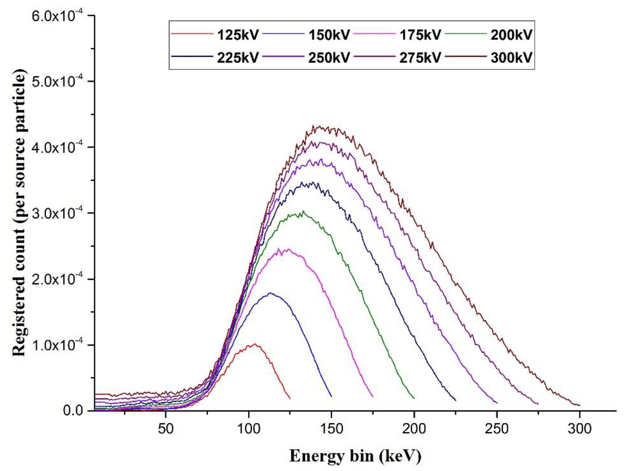
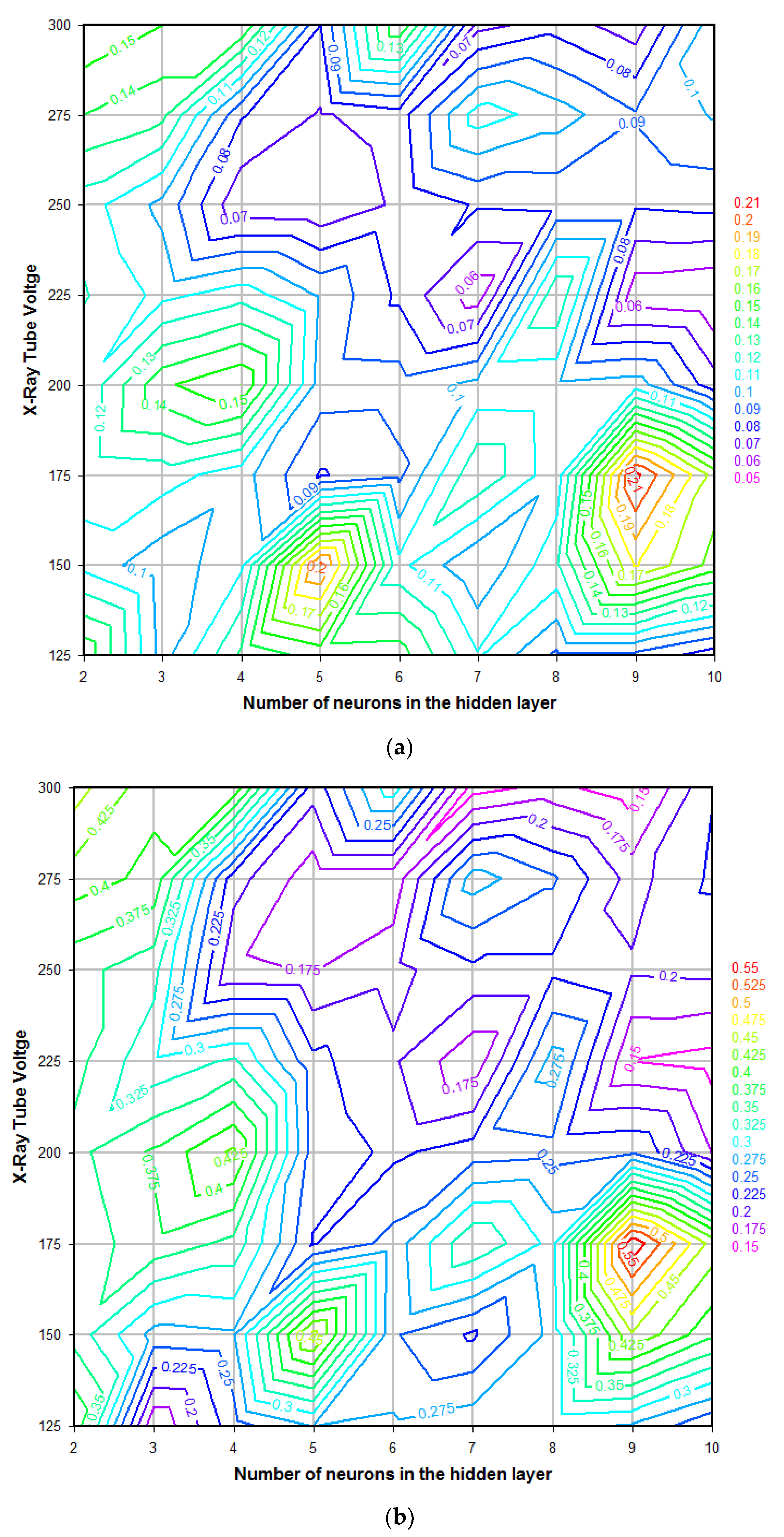
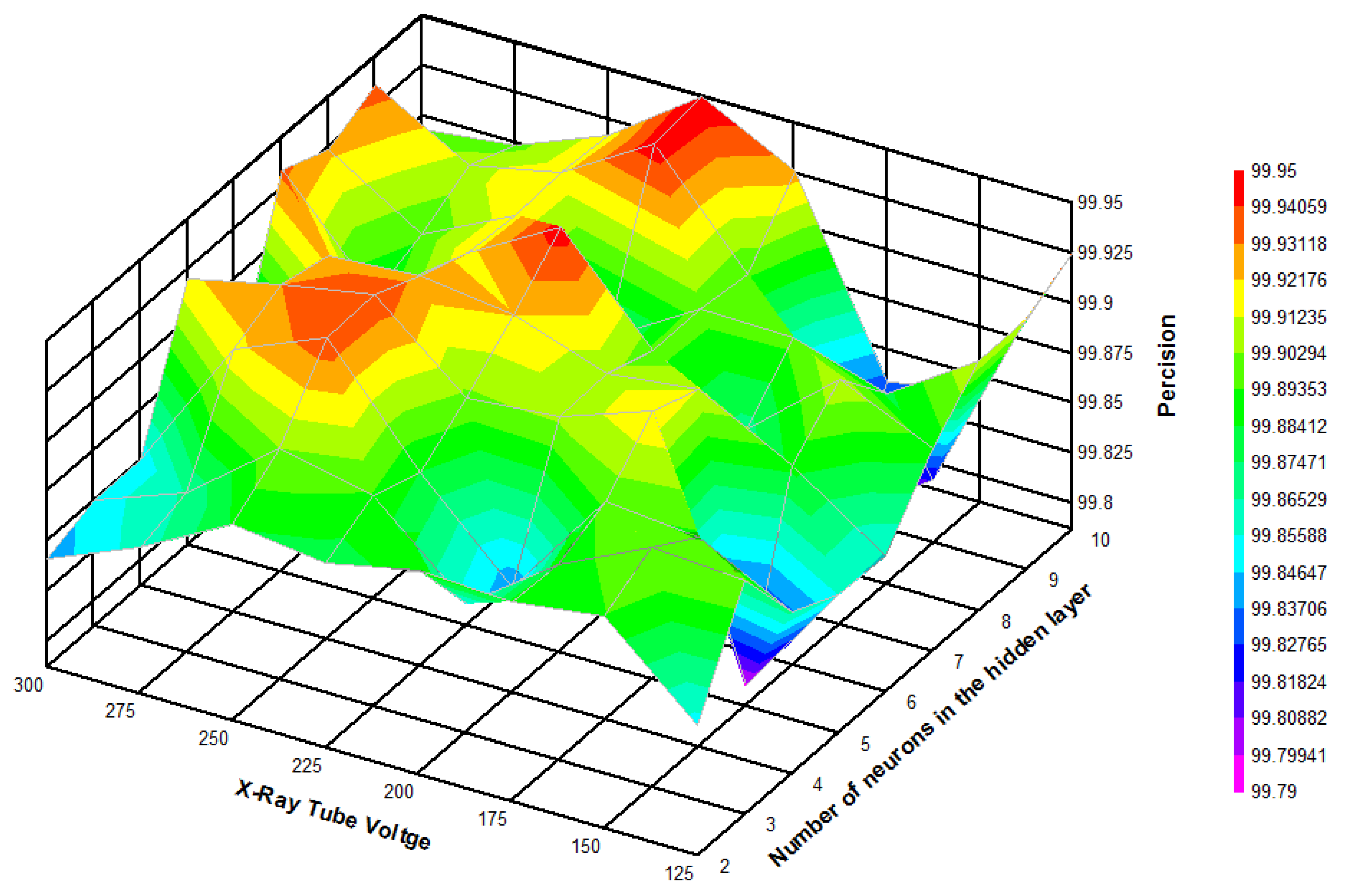
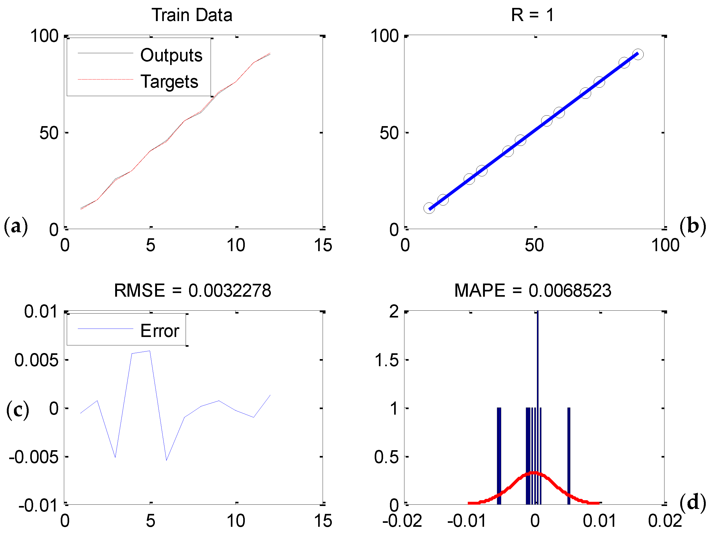
| Tube Voltage | 1 Neuron | 2 Neurons | 3 Neurons | 4 Neurons | 5 Neurons | 6 Neurons | 7 Neurons | 8 Neurons | 9 Neurons | 10 Neurons | |
|---|---|---|---|---|---|---|---|---|---|---|---|
| 125 | MAE train | 5.106 | 0.21 | 0.114 | 0.105 | 0.102 | 0.102 | 0.084 | 0.04 | 0.036 | 0.03 |
| MRE train (%) | 15.562 | 0.815 | 0.47 | 0.443 | 0.424 | 0.424 | 0.245 | 0.112 | 0.098 | 0.087 | |
| MAE test | 3.852 | 0.148 | 0.096 | 0.132 | 0.144 | 0.145 | 0.111 | 0.088 | 0.087 | 0.074 | |
| MRE test (%) | 8.022 | 0.398 | 0.151 | 0.239 | 0.275 | 0.279 | 0.291 | 0.28 | 0.272 | 0.228 | |
| 150 | MAE train | 5.223 | 0.146 | 0.143 | 0.085 | 0.068 | 0.045 | 0.032 | 0.014 | 0.007 | 0.002 |
| MRE train (%) | 15.977 | 0.657 | 0.624 | 0.44 | 0.338 | 0.142 | 0.069 | 0.036 | 0.021 | 0.006 | |
| MAE test | 3.958 | 0.107 | 0.093 | 0.108 | 0.203 | 0.113 | 0.09 | 0.118 | 0.181 | 0.156 | |
| MRE test (%) | 8.212 | 0.341 | 0.266 | 0.272 | 0.459 | 0.253 | 0.221 | 0.283 | 0.447 | 0.381 | |
| 175 | MAE train | 5.316 | 0.163 | 0.158 | 0.157 | 0.075 | 0.069 | 0.049 | 0.027 | 0.02 | 0.002 |
| MRE train (%) | 16.302 | 0.708 | 0.651 | 0.659 | 0.226 | 0.219 | 0.176 | 0.069 | 0.053 | 0.005 | |
| MAE test | 4.006 | 0.113 | 0.115 | 0.104 | 0.079 | 0.088 | 0.129 | 0.103 | 0.213 | 0.166 | |
| MRE test (%) | 8.313 | 0.331 | 0.368 | 0.343 | 0.223 | 0.259 | 0.35 | 0.291 | 0.571 | 0.44 | |
| 200 | MAE train | 5.403 | 0.179 | 0.107 | 0.062 | 0.044 | 0.025 | 0.017 | 0.01 | 0.01 | 0.004 |
| MRE train (%) | 16.585 | 0.729 | 0.386 | 0.306 | 0.133 | 0.07 | 0.053 | 0.033 | 0.033 | 0.009 | |
| MAE test | 4.075 | 0.111 | 0.148 | 0.16 | 0.095 | 0.094 | 0.103 | 0.102 | 0.105 | 0.074 | |
| MRE test (%) | 8.426 | 0.342 | 0.379 | 0.43 | 0.24 | 0.22 | 0.237 | 0.243 | 0.249 | 0.174 | |
| 225 | MAE train | 5.458 | 0.165 | 0.156 | 0.138 | 0.04 | 0.041 | 0.034 | 0.019 | 0.005 | 0.002 |
| MRE train (%) | 16.769 | 0.733 | 0.672 | 0.639 | 0.16 | 0.153 | 0.118 | 0.057 | 0.011 | 0.006 | |
| MAE test | 4.113 | 0.121 | 0.107 | 0.116 | 0.099 | 0.078 | 0.054 | 0.13 | 0.053 | 0.05 | |
| MRE test (%) | 8.498 | 0.359 | 0.305 | 0.33 | 0.232 | 0.204 | 0.154 | 0.286 | 0.149 | 0.14 | |
| 250 | MAE train | 5.52 | 0.154 | 0.142 | 0.052 | 0.053 | 0.035 | 0.026 | 0.015 | 0.006 | 0.006 |
| MRE train (%) | 16.95 | 0.684 | 0.625 | 0.15 | 0.152 | 0.121 | 0.1 | 0.048 | 0.014 | 0.015 | |
| MAE test | 4.16 | 0.115 | 0.097 | 0.062 | 0.061 | 0.072 | 0.081 | 0.082 | 0.081 | 0.083 | |
| MRE test (%) | 8.54 | 0.359 | 0.335 | 0.178 | 0.174 | 0.192 | 0.219 | 0.219 | 0.203 | 0.206 | |
| 275 | MAE train | 5.59 | 0.163 | 0.122 | 0.071 | 0.059 | 0.035 | 0.025 | 0.023 | 0.017 | 0.009 |
| MRE train (%) | 17.158 | 0.691 | 0.487 | 0.248 | 0.185 | 0.082 | 0.064 | 0.059 | 0.044 | 0.016 | |
| MAE test | 4.194 | 0.14 | 0.133 | 0.081 | 0.069 | 0.075 | 0.115 | 0.105 | 0.091 | 0.101 | |
| MRE test (%) | 8.608 | 0.413 | 0.393 | 0.211 | 0.16 | 0.158 | 0.287 | 0.254 | 0.19 | 0.229 | |
| 300 | MAE train | 5.637 | 0.18 | 0.151 | 0.114 | 0.094 | 0.07 | 0.039 | 0.021 | 0.009 | 0.007 |
| MRE train (%) | 17.347 | 0.755 | 0.59 | 0.517 | 0.313 | 0.172 | 0.097 | 0.043 | 0.03 | 0.0262 | |
| MAE test | 4.224 | 0.159 | 0.15 | 0.15 | 0.08 | 0.15 | 0.066 | 0.076 | 0.064 | 0.107 | |
| MRE test (%) | 8.66 | 0.462 | 0.407 | 0.42 | 0.21 | 0.317 | 0.139 | 0.159 | 0.133 | 0.224 |
Publisher’s Note: MDPI stays neutral with regard to jurisdictional claims in published maps and institutional affiliations. |
© 2021 by the authors. Licensee MDPI, Basel, Switzerland. This article is an open access article distributed under the terms and conditions of the Creative Commons Attribution (CC BY) license (https://creativecommons.org/licenses/by/4.0/).
Share and Cite
Alanazi, A.K.; Alizadeh, S.M.; Nurgalieva, K.S.; Grimaldo Guerrero, J.W.; Abo-Dief, H.M.; Eftekhari-Zadeh, E.; Nazemi, E.; Narozhnyy, I.M. Optimization of X-ray Tube Voltage to Improve the Precision of Two Phase Flow Meters Used in Petroleum Industry. Sustainability 2021, 13, 13622. https://doi.org/10.3390/su132413622
Alanazi AK, Alizadeh SM, Nurgalieva KS, Grimaldo Guerrero JW, Abo-Dief HM, Eftekhari-Zadeh E, Nazemi E, Narozhnyy IM. Optimization of X-ray Tube Voltage to Improve the Precision of Two Phase Flow Meters Used in Petroleum Industry. Sustainability. 2021; 13(24):13622. https://doi.org/10.3390/su132413622
Chicago/Turabian StyleAlanazi, Abdullah K., Seyed Mehdi Alizadeh, Karina Shamilyevna Nurgalieva, John William Grimaldo Guerrero, Hala M. Abo-Dief, Ehsan Eftekhari-Zadeh, Ehsan Nazemi, and Igor M. Narozhnyy. 2021. "Optimization of X-ray Tube Voltage to Improve the Precision of Two Phase Flow Meters Used in Petroleum Industry" Sustainability 13, no. 24: 13622. https://doi.org/10.3390/su132413622
APA StyleAlanazi, A. K., Alizadeh, S. M., Nurgalieva, K. S., Grimaldo Guerrero, J. W., Abo-Dief, H. M., Eftekhari-Zadeh, E., Nazemi, E., & Narozhnyy, I. M. (2021). Optimization of X-ray Tube Voltage to Improve the Precision of Two Phase Flow Meters Used in Petroleum Industry. Sustainability, 13(24), 13622. https://doi.org/10.3390/su132413622


