Abstract
Reverse logistics planning plays a crucial role in supply chain management. Stochasticity in different parameters along with time horizon can be a challenge in solving reverse logistics problems. This paper proposes a multi-stage, multi-period reverse logistics with lot sizing decisions under uncertainties. The main uncertain factors are return and demand quantities, and return quality. Moment matching method was adopted to generate a discrete set of scenarios to represent the original continuous distribution of stochastic parameters. Fast forward selection algorithm was employed to select the most representative scenarios and facilitate computational tractability. A case study was conducted and optimal solution of the recursive problem obtained by solving extensive form. Sensitivity analysis was implemented on different elements of stochastic solution. Results sow that solution of recursive problem (RP) outperforms the solution obtained from the problem with expected values of uncertain parameters (EEV).
1. Introduction
Reverse logistics problem is one of the most challenging problems in supply chain management (SCM) which aims to address collecting used, refurbished, or defective products from customers or primary markets and then carrying out some recovery and disposal activities Govindan et al. [1]. According to American Reverse Logistics Executive Council, reverse logistics is defined as “The process of planning, implementing, and controlling the efficient, cost effective flow of raw materials, in-process inventory, finished goods and related information from the points of consumption to the point of origin for the purpose of recapturing value or proper disposal”. Another report shows 7 million tonnes E-waste were generated across world annually ([2]). The amount of waste generated across the world increases the importance of reverse logistics systems in decreasing waste rate and return the leftover(s) to supply chain.
By reviewing body literature of the reverse logistics in deterministic and stochastic environments and review papers ([1,3,4]) the following gaps are recognized: Firstly, little attention has been paid to multi-echelon, multi-period stochastic reverse logistics with lot sizing. Secondly, multi-stage stochastic programming models for reverse logistics problem has not been investigated. Thirdly, to the best of our knowledge, the solution techniques introduced to solve stochastic reverse logistics problems are not efficient to solve large-scale instances which include large number of scenarios, stages, and decision variables. Stochasticty of several parameters of the problem along with time horizon complexity, makes multi-stage stochastic programming a good choice as a solution method for the mentioned gaps.
This study proposes a multi-stage stochastic program for multi-echelon, multi period reverse logistics program with lot sizing. Scenario generation and scenario reduction methods were employed to generate a representative set of discrete scenarios for underlying distribution of stochastic parameters. Extensive form of problem was used to solve the problem and stochastic solution was evaluated by implementing sensitivity analysis on recursive problem’s parameters.
2. Literature Review
Reverse logistics has been gaining popularity in recent years. A great portion of reverse logistics literature has been devoted to deterministic reverse logistics problems. Ref. [5] formulated a multi-stage reverse logistics network for product recovery as a mixed integer linear programming model. The authors validated the model with a used refrigerator recovery network. Ref. [6] developed a nonlinear mixed-integer linear programming model for a reverse logistics network which makes decisions on the number and locations of centralized return centers. They proposed a genetic algorithm to solve the formulated model. Ref. [7] proposed a mathematical model for a multi-stage, multi-product reverse logistics network. The authors developed a hybrid heuristic based on genetic algorithm for solving the introduced model. Ref. [8] studied a reverse logistics network for a company located in Brazil. They developed a returnable packaging model which decreases material consumption by 18% compared to disposable packaging model. In addition, they concluded that returnable packaging model is the best alternate in terms of environmental concerns since it has less environmental impacts compared to disposable packaging models. Ref. [9] addressed a reverse logistics network for end-of-live vehicles in Turkey. The authors proposed a mixed-integer linear programming model for the network. Solving the model led to the optimal number of facilities to be located. Ref. [10] formulated a reverse logistics network for a case of household appliance in the Gulf Cooperation Council (GCC) region with 68 cities. The authors developed a genetic algorithm with running time reduction up to 38 times compared to GMAS in solving the problem. Ref. [11] studied a multi-echelon capacitated reverse logistics network with location-routing, and time window constraints. The authors formulated the problem as a bi-objective mathematical programming model and proposed a non-dominated sorting genetic algorithm II (NSGA II) to obtain Pareto frontier solutions.
Compared to traditional forward logistics, more activities are involved in reverse logistics planning which makes it more challenging. One of the challenges in designing reverse logistics network is the presence of several uncertain factors such as return and demand quantities, and return quality. Therefore considering uncertainty and designing a robust decision making framework are crucial for reverse logistics design. Ref. [12] combined queuing models with traditional reverse logistics models to incorporate lead time and inventory positions in an uncertain environment. This combination led to a mixed integer nonlinear programming model. The authors solved the formulated model by a genetic algorithm with the technique of differential evolution. While most of the studied models in reverse logistics are case based, ref. [13] proposed a generalized model considering capacity limits, multi-product management, and uncertainty in demand and return quantities. They solved the formulated model by standard branch and bound techniques. Ref. [14] studied a risk-averse, two-stage stochastic programming approach reverse logistic network design problem. They considered return quantity and price as two sources of uncertainty. Ref. [15] focused on a reverse logistics problem with decisions on inventory control and production planning. They considered return and demand quantities as two stochastic parameters and modelled them using fuzzy trapezoidal numbers. The authors developed a two phase fuzzy mixed integer optimization algorithm to solve the formulated model. Ref. [16] studied a reverse logistics network with three uncertainty sources: return quantity, return quality, and transportation cost. They formulated the problem as a two-stage stochastic programming model and validated it by a real world case for waste of electrical and electronic equipment recycling center in Turkey. The authors used sample average approximation method to solve the model. Ref. [17] proposed a dynamic location and allocation model for reverse logistic problem and formulated it as a two stage stochastic programming model. Also, they developed a heuristic solution method based on sampling to solve the model. Ref. [18] studied a multi-period reverse logistics network under return and demand uncertainty with lot sizing and formulated it as a two-stage stochastic programming model. They used scenario generation and scenario reduction methods to generate sets of discrete scenarios to approximate underlying probability distributions. The authors used a case of consumer company in Europe to validate the proposed model. Ref. [19] designed an International Reverse Logistics (IRL) network under uncertainty. Authors used Japanese case study to formulate a resilient and efficient IRL model to minimize the total cost of system subject to resilience constraints. Ref. [20] designed a two-stage stochastic programming model for eco-efficient reverse logistics problem to minimize landfilling activities and maximize expected profit. In their study, recycling rates and the quantity of generated waste are considered as two main sources of uncertainties. Authors implemented Sampling Average Approximation process and -constrained method to solve the formulated problem. They used a wood waste recycling case study in province of Quebec in Canada. Ref. [21] designed a reverse logistics network for recycling construction and demolition wastes. They proposed a multi-objective, multi-period mixed integer programming model for this network design problem. Authors included two uncertain factors in this reverse logistics network: rate of investment and recycled products demand. Risk averse two-stage stochastic programming model was used to solve the model under uncertainty. Ref. [22] present a stochastic mixed integer programming model for designing and planning a generic multi-source, multi-echelon, capacitated, and sustainable reverse logistics network for WEEE management under uncertainty. Their model takes into account both economic efficiency and environmental impacts in decision-making, and the environmental impacts are evaluated in terms of carbon emissions. Authors employed a multi-criteria two-stage scenario-based solution method for generating the optimal solution for the stochastic optimization problem. Ref. [23] models the electrical and electronic equipment (EEE) reverse logistics process as a bi-objective mixed-integer programming model under uncertainties. Their mathematical model investigates two objectives: an economic objective and an environmental objective. The first is minimizing cost, while the second is maximizing the environmental score by reverse logistics processes in recovering and recycling. The parameters of demand and WEEE return rate which is obtained from the customer were considered as two uncertain parameters. Ref. [24] identifies reverse logistics barriers through (1) an extent literature review, (2) advice from Bangladeshi industry experts under the Delphi study, and (3) ranking reverse logistics barriers using the fuzzy analytical hierarchy process. The results indicate that, of the barriers investigated, the ‘knowledge and support’ category seems to be most critical. A lack of interest and support from top-level management—related to ‘knowledge and support’ issues—appears to be the major obstacle for reverse logistics implementation in the Bangladeshi leather footwear industry. Ref. [25] applied Interpretive Structural Modeling (ISM) technique to diagnose significant barriers and proposed a hierarchical framework for investigating the relationships among them. They used MICMAC (Matriced’ Impacts Croisés Multiplication Appliquée á unClassement) analysis to classify the barriers based on the driving power and dependence among them.
The reminder of this paper is organized as follows: Section 3 provides describes reverse logistics network problem with lot-sizing and under uncertainty and proposes a multi-stage stochastic programming model for this problem. Section 4 conducts a case study and Section 5 discusses computational results and sensitivity analysis. Section 6 provides conclusions and proposes future research directions.
3. Problem Statement
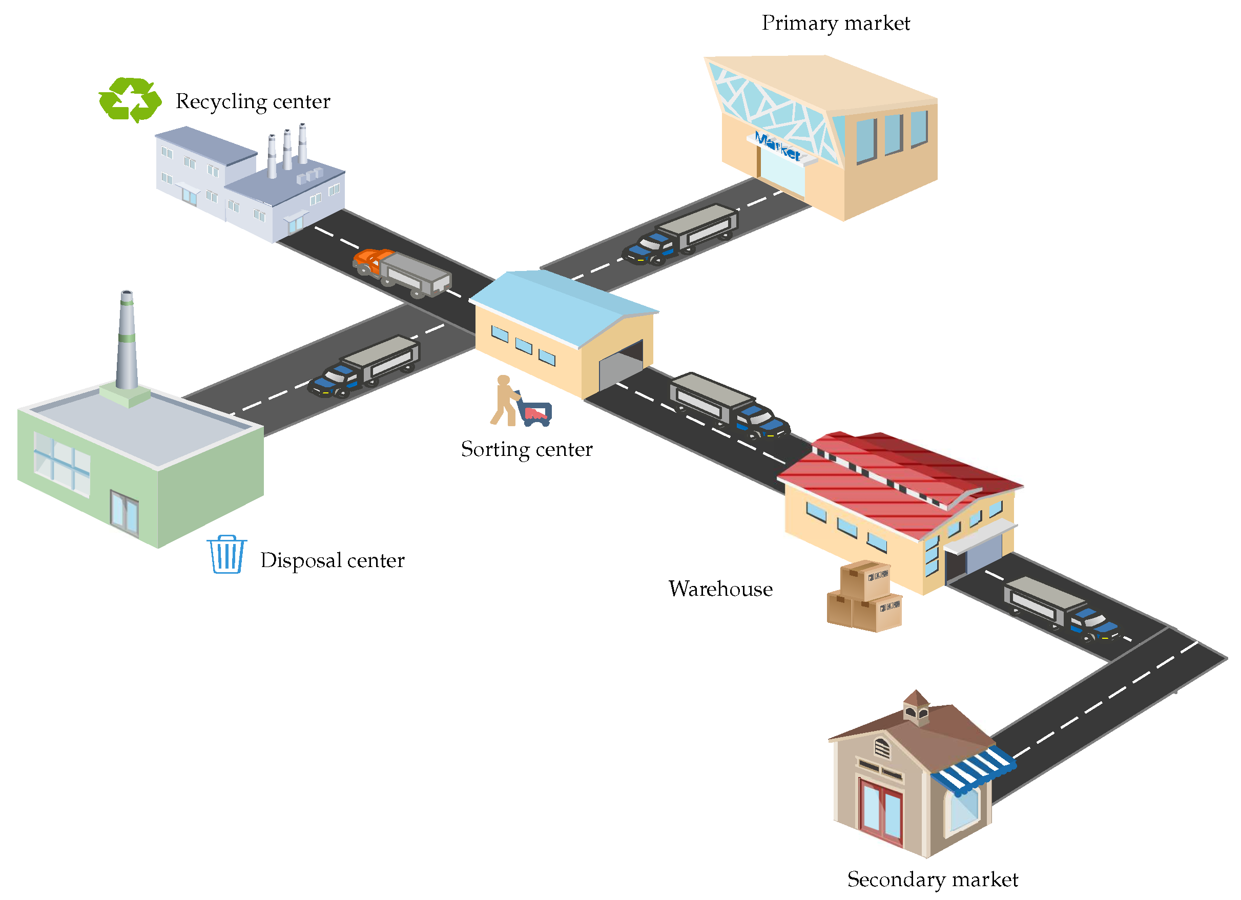
In the reverse logistics network considered in this research, returned products flow from primary markets as upstream level to sorting centers. After screening products at sorting centers, the products are sorted to three groups. The products with good quality are transported to warehouses to meet secondary markets’ demand. The products with lower quality level that are recyclable will be transported to recycling centers. The rest of the returned products will be transported to disposal centers. During these processes, return and demand quantities, and quality level are the main sources of uncertainty. In this study, we formulate and solve multi-echelon, multi-period reverse logistics problem as a multi-stage stochastic programming model. In fact, this study provides a diagram for decision makers to make the optimal decisions on (1) locating facilities such as sorting centers, recycling centers, and disposal centers; (2) the amount of products should be transported between different facilities and from facilities to secondary markets as final customers; (3) inventory, outsourcing, backorder, and shortage levels. Structure of network is illustrated in Figure 1.

Figure 1.
Network structure.
3.1. Model Formulation
This section introduces the proposed multi-stage stochastic programming model.
Assumptions are listed as follows:
- Inventory in sorting centers, recycling centers, and disposal centers are not allowed.
- Initial inventory is not allowed in warehouses.
- End of each period is set to measure inventory level of warehouses.
- Fulfilling of secondary markets’ demand can be delayed or ignored since backorders and shortages are allowed.
- Transportation between the same kind of facilities are not allowed (e.g., transportation between warehouses is prohibited).
The notations of the model formulation are as following.
3.1.1. Objective Function
The objective function minimizes the total expected costs of network including establishment costs (), transportation costs (), inventory costs (), backorder costs (), shortage costs (), and outsourcing costs () over the planning horizon. Equations (1)–(7) present the objective function and its elements:
In Equation (2), the four terms include all first stage decision variables and represent location cost for sorting centers, warehouses, recycling centers, and disposal centers, respectively. Equation (3), with five terms, calculates transportation costs of primary markets to sorting center, sorting centers to warehouses, sorting centers to recycling centers, sorting centers to disposal centers, and warehouses to secondary markets, respectively. Equation (7) includes outsourcing costs for sorting centers, warehouses, recycling centers, and disposal centers.
3.1.2. Constraints
This section discusses constraints in detail.
Constraints (8)–(12) are related to capacities of facilities and transportation amount between the facilities. These constraints prohibit product flows between facilities that are not established. Meanwhile, capacities for the facilities can not be exceeded.
Constraints (13) state that the amount of return products from primary markets include transported products to sorting centers and the amount of returned products which exceed sorting centers’ capacity.
Constraints (14)–(16) calculate the transported amount of products from sorting centers to recycling centers, disposal centers, and warehouses, respectively. At the same time, these constraints calculate the amount of products exceeding the capacities of these facilities.
Constraints (17)–(20) state outsourcing is not allowed from facilities that are not established.
Constraints (21)–(23) determine the inventory level at each warehouse.
Constraints (24)–(26) determine the amount of product transported to each secondary market.
Constraints (27) state transportation flows between warehouses are not allowed.
Constraints (28) calculate backorder level for each secondary market.
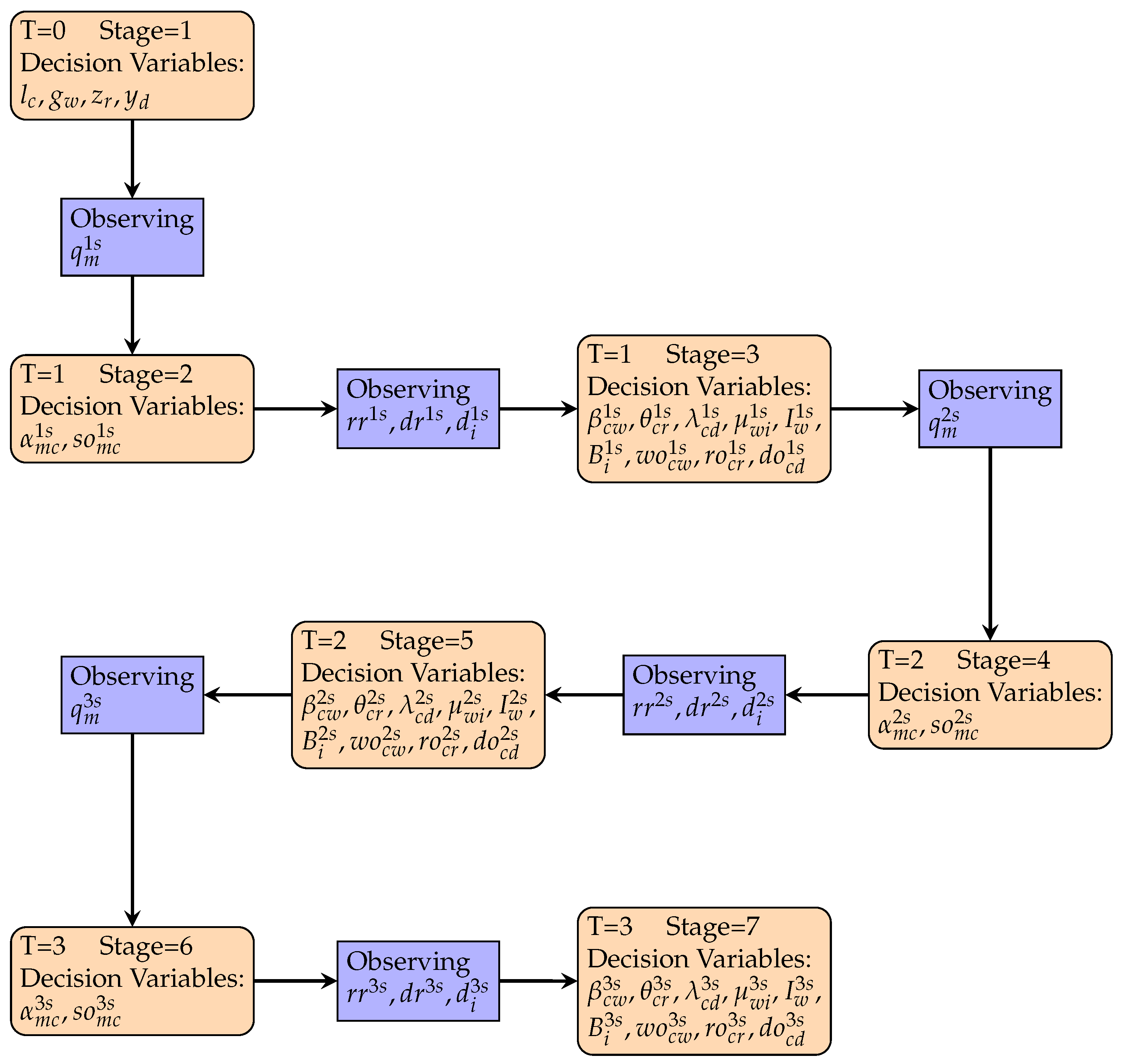
Figure 2 shows the different decision making stages and their associated decision variables in the problem.

Figure 2.
Decision making process in different stages.
4. Case Study
To validate the proposed multi-stage stochastic programming model, a case study adapted from [26] was applied. Ref [26] developed a deterministic mixed integer linear program for the case of a European consumer goods company. This study extended their work by proposing multi-echelon, multi-period, and multi-stage stochastic program for reverse logistics network.
The network logistics of this case consists of 38 nodes distributed in different European countries including five primary markets, six potential candidates for sorting centers, three potential candidates for warehouses, three potential candidates for recycling centers, three potential candidates for disposal centers, and eighteen secondary market nodes.
Table 1 reports the facilities capacities and establishment costs. Table 2 lists the unit holding cost, unit backorder cost, and unit shortage cost. Quantities of returned products from the primary markets and demand of secondary markets are assumed to follow normal distributions (Abdallah et al. (2012)). Four moments of return and demand quantities distributions are reported in Table 3 and Table 4, respectively. Return quantities in different time periods are assumed independent from each other. Demand quantities are also independent from each other in different time periods. The rates of recyclable and disposable products are the other stochastic parameters with five possible outputs listed in Table 5. The planning horizon for this research problem is considered to be three months and outsourcing cost per unit of product for all facilities is assumed to be 30 rmu.

Table 1.
Establishing cost (EC) and Capacity (Cap).
Table 2.
Costs of holding, backorder and shortage per unit of product.
Table 3.
Return properties.
Table 4.
Demand properties.
Table 5.
Rate of recycling and disposal.
5. Results and Analysis
The most effective method to solve small to medium size stochastic programs is to generate the deterministic equivalent of the problem so-called extensive form. Extensive form specifies all scenarios in one single mathematical model.
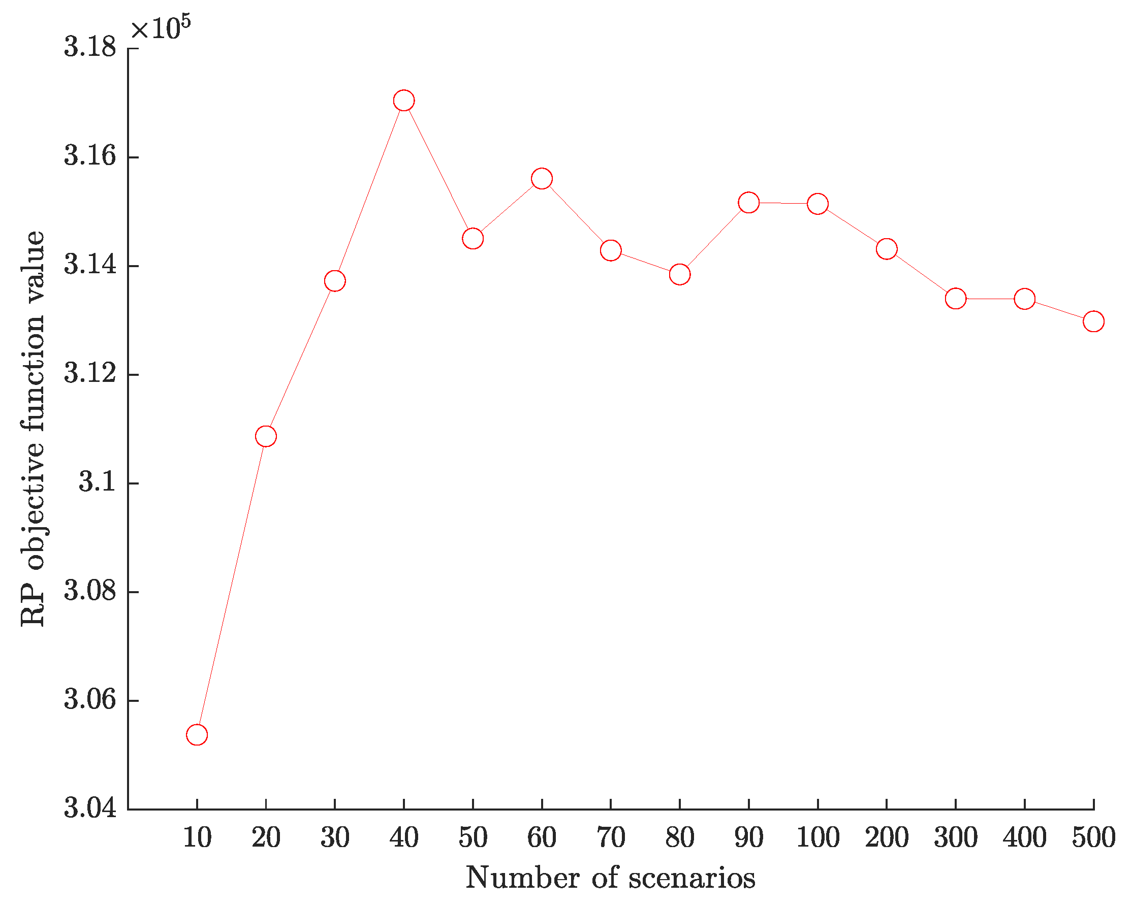
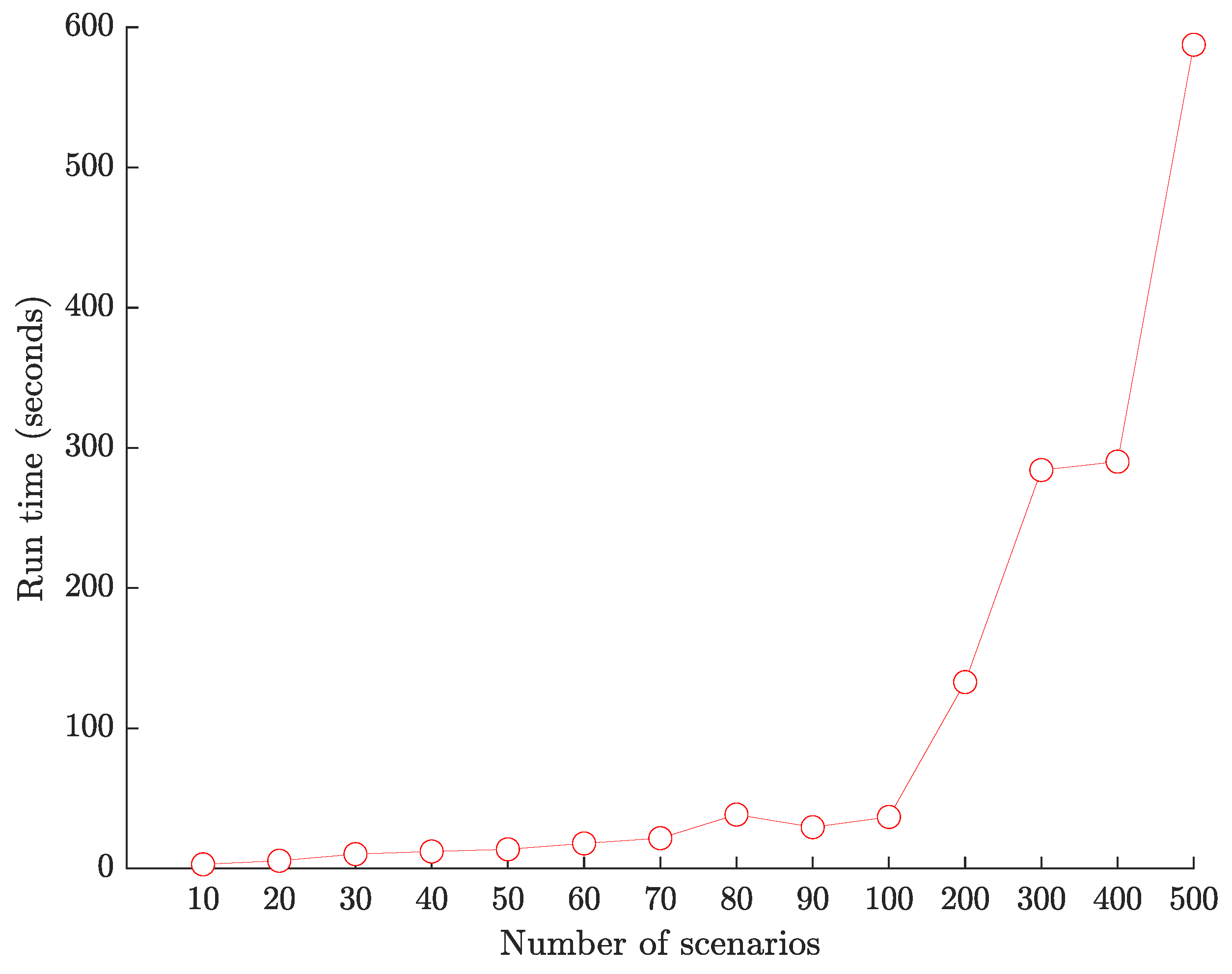
Section 3 provided extensive form mathematical model of the introduced problem. To solve the problem in extensive form, discrete scenarios are generated by moment matching method and then the total number of scenarios is reduced by fast forward selection algorithm. Scenario generation and scenario reduction were implemented in GAMS 23.5 to create the most representative scenarios for the stochastic problem. The scenarios data files for the problem was generated by Matlab R2020b and stochastic program was coded in Python 3.7 to solve and find the optimal solution. Optimal solution for a relatively small-scale instance with 5 scenario is listed in Table 6 and Table 7. Figure 3 shows the objective function value of extensive form for cases with 10 to 500 scenarios. As it can be seen from this figure, the total cost is gradually converging by increasing number of scenarios from 50 up to 500. For analyzing experimental results the case with 300 scenarios is considered. Figure 4 shows the run time of the cases with different number of scenarios. As expected, the run time increases by increasing number of scenarios.
Table 6.
First stage decision variables values.
Table 7.
Extensive form results ().
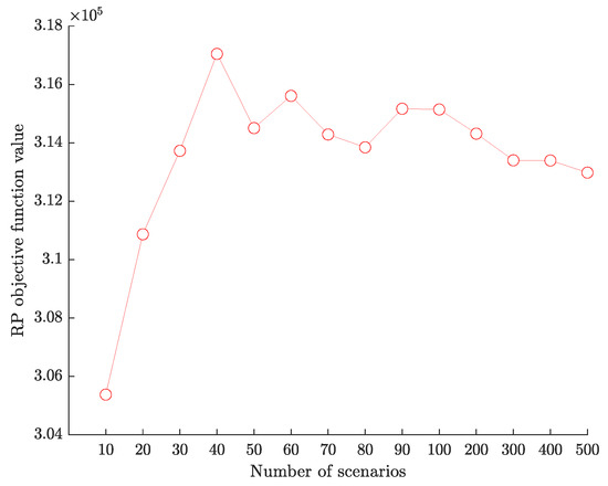
Figure 3.
Total cost of the system.
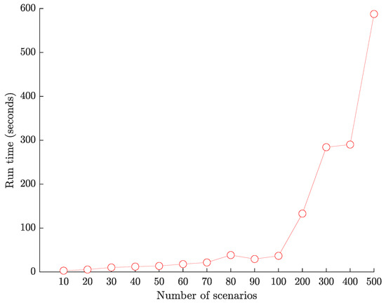
Figure 4.
Run time for different number of scenarios.
To evaluate the quality of stochastic solution, the model is solved for EV (Expected Value), EEV (Expected problem of Expected Value solution), and RP (Recourse Problem) are solved. EV problem assigns fixed values to stochastic parameters. The fixed value is the mean of distribution for each stochastic parameter. In other words, EV problem ignores stochasticity but stochasticity exists and what will happen in reality (EEV solution) is different from the optimum solution of EV. EEV problem solves the formulation by fixing first stage variables with the solution obtained from EV problem. Table 8 shows the solutions obtained by solving EV, EEV, and RP. The value of stochastic solution (VSS) is the difference between EEV and RP which in this case is 12,516.7 indicating RP solution outperforms EEV solution.
Table 8.
EV, EEV, and RP problems results.
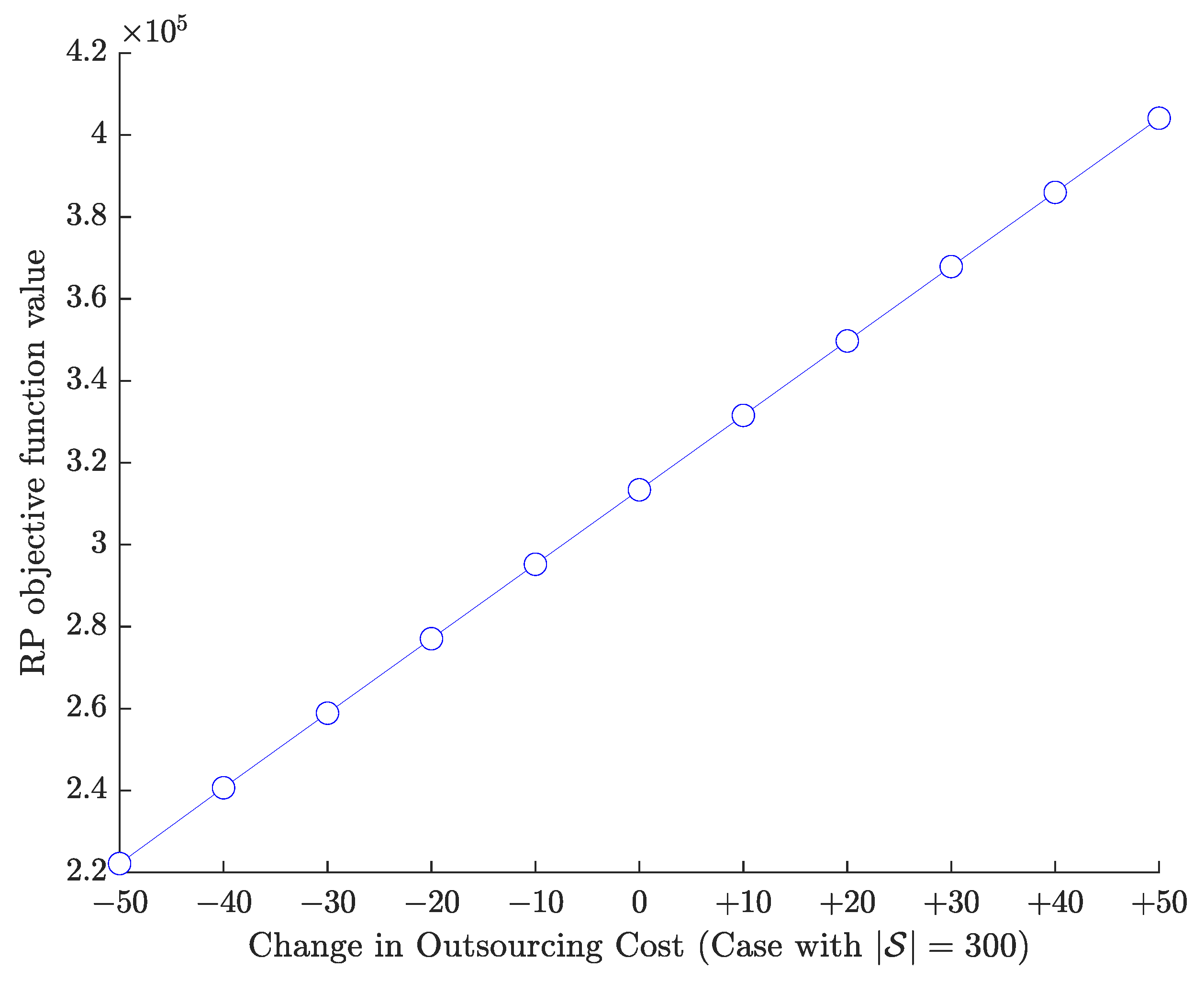
In the next step we do a sensitivity analysis in outsourcing cost (OC) which is one the important elements in total cost of system. Figure 5 shows the change in total cost by decreasing or increasing OC. Linear relationship between OC and objective function value indicates no change in other cost elements of objective function which means optimal solution is not changing by change in OC. Since total demand of secondary markets is less than total return of primary markets, final solution always includes outsourced extra returned items.
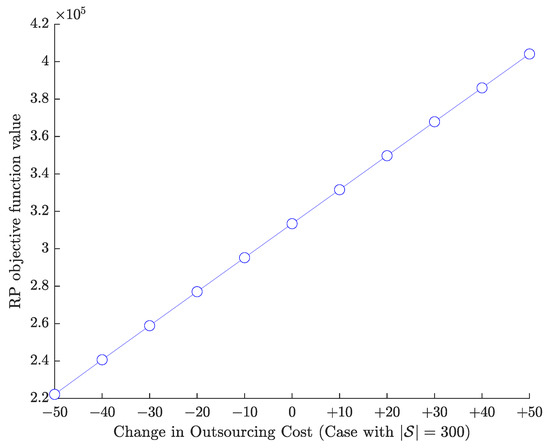
Figure 5.
Sensitivity Analysis on Outsourcing Cost (OC).
6. Conclusions
Traditional supply chain design considers product flow from suppliers to customers. However in reverse logistics problem as a supply chain problem, the product flow starts from customers(primary markets) and end at manufacturers(secondary markets). Decision making in such environments face several uncertainty factors. Recently, designing a reverse logistics network involved in stochastic environment has attracted more attention in the literature.
In this paper, we design a reverse logistics network by formulating it as a multistage stochastic programming model. Uncertainty sources in this problem include return quantity in primary markets, demand quantity in secondary markets, recycling rate, and disposal rate. The first two uncertainty sources have normal distribution. Hence, moment matching method was used as a scenario generation approach to create discrete scenarios. Then fast forward selections was applied to decrease the number of scenarios. Finally extensive form of the formulation was solved to find the optimal solution of stochastic problem and sensitivity analysis was implemented to get managerial insights. Scenario reduction algorithm reduced run time while quality of solution is reasonable. Also, RP solution outperforms EEV solution which shows applicability of multi-stage stochastic programming approach for similar environments. This study is subject to to a few limitations which suggest some future research directions. First, considering return quality as a continuous variable would be desirable in finding the optimal solution. Second, usually real-life cases might be in a large-scale form. So, developing exact and heuristic algorithms to solve the large-scale problems can be appealing. Last but not the least, developing valid inequalities is crucial in decreasing the time complexity of the problem for large scale instances.
Author Contributions
Data curation, V.A.; Formal analysis, V.A.; Funding acquisition, G.H.; Methodology, V.A. and G.H.; Project administration, G.H. All authors have read and agreed to the published version of the manuscript.
Funding
This research received no external funding.
Institutional Review Board Statement
Not applicable.
Informed Consent Statement
Not applicable.
Data Availability Statement
Not applicable.
Conflicts of Interest
The authors declare no conflict of interest.
Abbreviations
| Sets | |
| Primary markets | |
| Candidate locations for sorting centers | |
| W | Candidate locations for warehouses |
| Secondary markets | |
| Union of warehouses and secondary markets, | |
| R | Candidate recycling centers |
| D | Candidate disposal centers |
| T | Time periods |
| S | Set of scenarios |
| Parameters | |
| Probability of scenario s | |
| Cost of establishing a sorting center in location c | |
| Cost of establishing a warehouse in location i | |
| Cost of establishing a recycling center in location r | |
| Cost of establishing a disposal center in location r | |
| Return quantity of primary market m in period t under scenario s | |
| Cost of transportation for one unit of product from primary market m to sorting center c | |
| Cost of transportation for one unit of product from sorting center c to warehouse w | |
| Cost of transportation for one unit of product from sorting center c to recycling center r | |
| Cost of transportation for one unit of product from sorting center c to disposal center d | |
| Cost of transportation for one unit of product from node to node | |
| Holding cost for one unit of product in warehouse w in period t | |
| Cost of backorder for one unit of product for secondary market i in period t | |
| Cost of shortage for one unit of unmet demand of secondary market i | |
| Cost of outsourcing for one unit of product | |
| Demand of secondary market i in period t under scenario s | |
| Ratio of disposal in period t under scenario s | |
| Ratio of recycling in period t under scenario s | |
| Sorting center c’s capacity | |
| Warehouse w’s capacity | |
| Recycling center r’s capacity | |
| Disposal center d’s capacity | |
| Decision Variables | |
| 1 if sorting center c established, 0 otherwise | |
| 1 if warehouse w is established, 0 otherwise | |
| 1 if disposal center d is established, 0 otherwise | |
| 1 if recycling center r is established, 0 otherwise otherwise | |
| Amount of products transported from primary market m to sorting center under scenario s in period t | |
| Amount of products transported from sorting center c to warehouse w under scenario s in period t | |
| Amount of products transported from sorting center c to recycling center r under scenario s in period t | |
| Amount of products transported from sorting center c to disposal center d under scenario s in period t | |
| Amount of products transported from warehouse w to secondary market i under scenario s in period t | |
| Inventory level of products in warehouse w under scenario s in period t | |
| Backordered demand for secondary market i under scenario s in period t | |
| Outsourced products of shipment from primary market m to sorting center c (because of capacity exceeding in sorting center c) under scenario s in period t | |
| Outsourced products of shipment from sorting center c to recycling center r (because of capacity exceeding in recycling center r) under scenario s in period t | |
| Outsourced products of shipment from sorting center c to disposal center d (because of capacity exceeding in disposal center d) under scenario s in period t | |
| Outsourced products of shipment from sorting center c to warehouse w (because of capacity exceeding in warehouse w) under scenario s in period t | |
| Cumulative total demand of secondary market i over t periods under scenario s, () | |
| Cumulative total shipment transported from warehouse w to secondary market i over t periods under scenario s, () | |
| Cumulative total backorder for secondary market i over t periods under scenario s, () | |
| Cumulative total shipment transported from sorting center c to warehouse w over t periods under scenario s, () |
References
- Govindan, K.; Fattahi, M.; Keyvanshokooh, E. Supply chain network design under uncertainty: A comprehensive review and future research directions. Eur. J. Oper. Res. 2017, 263, 108–141. [Google Scholar] [CrossRef]
- Balde, C.P.; Wang, F.; Kuehr, R.; Huisman, J. The Global e-Waste Monitor 2014: Quantities, Flows and Resources; United Nations University, International Telecommunication Union, and International Solid Waste Association: Bonn, Germany, 2015. [Google Scholar]
- Prajapati, H.; Kant, R.; Shankar, R. Bequeath life to death: State-of-art review on reverse logistics. J. Clean. Prod. 2019, 211, 503–520. [Google Scholar] [CrossRef]
- Rachih, H.; Mhada, F.Z.; Chiheb, R. Meta-heuristics for reverse logistics: A literature review and perspectives. Comput. Ind. Eng. 2019, 127, 45–62. [Google Scholar] [CrossRef]
- John, S.T.; Sridharan, R.; Kumar, P.R.; Krishnamoorthy, M. Multi-period reverse logistics network design for used refrigerators. Appl. Math. Model. 2018, 54, 311–331. [Google Scholar] [CrossRef]
- Min, H.; Ko, H.J.; Ko, C.S. A genetic algorithm approach to developing the multi-echelon reverse logistics network for product returns. Omega 2006, 34, 56–69. [Google Scholar] [CrossRef]
- Lee, J.E.; Gen, M.; Rhee, K.G. Network model and optimization of reverse logistics by hybrid genetic algorithm. Comput. Ind. Eng. 2009, 56, 951–964. [Google Scholar] [CrossRef]
- Silva, D.A.L.; Reno, G.W.S.; Sevegnani, G.; Sevegnani, T.B.; Truzzi, O.M.S. Comparison of disposable and returnable packaging: A case study of reverse logistics in Brazil. J. Clean. Prod. 2013, 47, 377–387. [Google Scholar] [CrossRef]
- Demirel, E.; Demirel, N.; Gökçen, H. A mixed integer linear programming model to optimize reverse logistics activities of end-of-life vehicles in Turkey. J. Clean. Prod. 2016, 112, 2101–2113. [Google Scholar] [CrossRef]
- Alshamsi, A.; Diabat, A. A Genetic Algorithm for Reverse Logistics network design: A case study from the GCC. J. Clean. Prod. 2017, 151, 652–669. [Google Scholar] [CrossRef]
- Ghezavati, V.; Beigi, M. Solving a bi-objective mathematical model for location-routing problem with time windows in multi-echelon reverse logistics using metaheuristic procedure. J. Ind. Eng. Int. 2016, 12, 469–483. [Google Scholar] [CrossRef] [Green Version]
- Lieckens, K.; Vandaele, N. Reverse logistics network design with stochastic lead times. Comput. Oper. Res. 2007, 34, 395–416. [Google Scholar] [CrossRef]
- Salema, M.I.G.; Barbosa-Povoa, A.P.; Novais, A.Q. An optimization model for the design of a capacitated multi-product reverse logistics network with uncertainty. Eur. J. Oper. Res. 2007, 179, 1063–1077. [Google Scholar] [CrossRef]
- Soleimani, H.; Govindan, K. Reverse logistics network design and planning utilizing conditional value at risk. Eur. J. Oper. Res. 2014, 237, 487–497. [Google Scholar] [CrossRef]
- Niknejad, A.; Petrovic, D. Optimisation of integrated reverse logistics networks with different product recovery routes. Eur. J. Oper. Res. 2014, 238, 143–154. [Google Scholar] [CrossRef]
- Ayvaz, B.; Bolat, B.; Aydın, N. Stochastic reverse logistics network design for waste of electrical and electronic equipment. Resour. Conserv. Recycl. 2015, 104, 391–404. [Google Scholar] [CrossRef]
- Lee, D.H.; Dong, M. Dynamic network design for reverse logistics operations under uncertainty. Transp. Res. Part E Logist. Transp. Rev. 2009, 45, 61–71. [Google Scholar] [CrossRef]
- Azizi, V.; Hu, G.; Mokari, M. A two-stage stochastic programming model for multi-period reverse logistics network design with lot-sizing. Comput. Ind. Eng. 2020, 143, 106397. [Google Scholar] [CrossRef]
- Sugimura, Y.; Murakami, S. Designing a Resilient International Reverse Logistics Network for Material Cycles: A Japanese Case Study. Resour. Conserv. Recycl. 2021, 170, 105603. [Google Scholar] [CrossRef]
- Trochu, J.; Chaabane, A.; Ouhimmou, M. A carbon-constrained stochastic model for eco-efficient reverse logistics network design under environmental regulations in the CRD industry. J. Clean. Prod. 2020, 245, 118818. [Google Scholar] [CrossRef]
- Rahimi, M.; Ghezavati, V. Sustainable multi-period reverse logistics network design and planning under uncertainty utilizing conditional value at risk (CVaR) for recycling construction and demolition waste. J. Clean. Prod. 2018, 172, 1567–1581. [Google Scholar] [CrossRef]
- Yu, H.; Solvang, W.D. A stochastic programming approach with improved multi-criteria scenario-based solution method for sustainable reverse logistics design of waste electrical and electronic equipment (WEEE). Sustainability 2016, 8, 1331. [Google Scholar] [CrossRef] [Green Version]
- Moslehi, M.S.; Sahebi, H.; Teymouri, A. A multi-objective stochastic model for a reverse logistics supply chain design with environmental considerations. J. Ambient Intell. Humaniz. Comput. 2020, 12, 8017–8040. [Google Scholar] [CrossRef]
- Moktadir, M.A.; Rahman, T.; Ali, S.M.; Nahar, N.; Paul, S.K. Examining barriers to reverse logistics practices in the leather footwear industry. Ann. Oper. Res. 2020, 93, 715–746. [Google Scholar] [CrossRef]
- Ali, S.M.; Arafin, A.; Moktadir, M.A.; Rahman, T.; Zahan, N. Examining barriers to reverse logistics practices in the leather footwear industry. Glob. J. Flex. Syst. Manag. 2018, 293, 53–68. [Google Scholar] [CrossRef]
- Kalaitzidou, M.A.; Longinidis, P.; Georgiadis, M.C. Optimal design of closed-loop supply chain networks with multifunctional nodes. Comput. Chem. Eng. 2015, 80, 73–91. [Google Scholar] [CrossRef]
Publisher’s Note: MDPI stays neutral with regard to jurisdictional claims in published maps and institutional affiliations. |
© 2021 by the authors. Licensee MDPI, Basel, Switzerland. This article is an open access article distributed under the terms and conditions of the Creative Commons Attribution (CC BY) license (https://creativecommons.org/licenses/by/4.0/).