Article

The Impact of Thin Asphalt Layers as a Road Traffic Noise Intervention in an Urban Environment

by
Ablenya Grangeiro de Barros
1,*,
Jarl K. Kampen
2,3 and
Cedric Vuye
1
1
EMIB Research Group, Faculty of Applied Engineering, University of Antwerp, 2020 Antwerp, Belgium
2
STATUA, Department of Epidemiology and Social Medicine, University of Antwerp, 2000 Antwerp, Belgium
3
Biometris, Wageningen University and Research Center, 6708 PB Wageningen, The Netherlands
*
Author to whom correspondence should be addressed.
Sustainability 2021, 13(22), 12561; https://doi.org/10.3390/su132212561
Submission received: 6 October 2021 / Revised: 7 November 2021 / Accepted: 9 November 2021 / Published: 13 November 2021
(This article belongs to the Special Issue Urban Noise)

Abstract

:
Low-noise thin asphalt layers (TALs) are a feasible solution to mitigate road traffic noise in urban environments. Nevertheless, the impacts of this type of noise intervention are reported mostly regarding noise levels, while non-acoustic aspects influencing the population perception are still little-known. This study investigates the implementation of TALs in two streets of Antwerp, Belgium. The effectiveness of the intervention was measured via noise modelling and acoustic measurements of road traffic noise. A reduction of 2.8 dB in noise exposure was observed in Lden and Lnight, while SPB measurements showed decreases up to 5.2 dB on the roadside. The subjective impacts of the TALs were evaluated via self-administered surveys and compared to results from control streets. The annoyance indicators were positively impacted by the TALs implementation, resulting in annoyance levels similar or lower than in the control streets. The TALs did not impact the reported physical complaints, sleep quality, and comfort level to perform activities.

1. Introduction

Road traffic noise is considered to be the second most prevailing environmental risk factor to human health, after fine particle pollution, especially in densely populated cities in Europe [1]. Even though air pollution emissions have been successfully reduced in the last decades, noise emission per vehicle has not changed considerably since the early seventies [2].
Long-term exposure to road traffic noise has been associated with non-auditory health outcomes such as cardiovascular diseases, cognitive dysfunction, sleep disorder, among others [3]. The build-up of somatic disease arises from physiological responses triggered by exposure to high levels of (road traffic) noise. These somewhat unconscious behavioral reactions to noise exposure can be subjectively measured by the “noise annoyance”. This indicator is assessed at the population level via social surveys and is more easily reported by the exposed population to describe (road traffic) noise exposure than the manifestation of somatic disease; see [4] for an elaborate review on this topic. Thus, annoyance could be considered an early warning signal for health risks, playing a key role in setting noise exposure limits and creating action plans for noise exposure mitigation [5].
In previous research, the objective noise levels were correlated with the subjective perception of noise, meaning the annoyance levels, in so-called exposure-response relationships (ERR) or functions (ERF) [4,6,7]. These large-scale ERRs result from the compilation of various studies that used different survey methods and noise level calculations. Using pre-defined ERRs reduces the cost and time to measure annoyance compared to conducting field surveys. On the other hand, calculating noise annoyance via ERRs may lead to inaccurate results, as these relations overlook non-acoustic factors of annoyance that can impact noise perception more than the noise level itself [8]. Some of the factors influencing annoyance level include noise source type (traffic, railroad or air) and personal aspects such as age, emotion [9], expectations regarding the noise [10] and noise sensitivity of the individual [11,12].
Besides the noise–exposure relationships, recent studies have tried to draw links between noise or annoyance levels to aspects of quality of life, well-being and mental health. Nevertheless, Pershagen et al. [13] remark that the understanding of adverse effects of environmental noise pollution on health has only advanced recently. A population-based cohort study [14] revealed that noise annoyance could predict depression, anxiety and sleep disturbance in a 5-year timeframe. For annoyance from road traffic noise in specific, sleep disturbance was consistently predicted. In ref. [15], it is suggested that high noise exposure levels (Lden > 60 dB) can lead to an increase in anxiolytic and anti-depressant use, especially when the bedroom windows face the street. The importance of having a window facing a quiet side was demonstrated earlier in [16,17]; it not only reduces the risk of annoyance and concentration problems but reduces sleeping problems in the case of a bedroom window. Ref. [18] found evidence to sustain that noise exposure is responsible for impairing children’s reading comprehension and long-term memory. Regarding cardiovascular health, there is suggestive evidence that transportation noise exposure is associated with an increase in ischemic heart disease [19], whereas these links are less consistent with diastolic blood pressure. Ref. [20] showed that higher levels of diastolic blood pressure are observed with increases of 5 dB (A) of night-time noise, while [21] found considerably higher effects of traffic noise exposure only among participants with physician-diagnosed hypertension and diabetes.
The Directive 2002/49/EC, known as the Environmental Noise Directive (END) [22], was implemented to guide the European Union Member States (EU MS) in assessing and managing environmental noise. The EU MS are required to perform strategic noise mapping for all major roads, railways, airports, and agglomerations on a 5-year basis [23]. This legal obligation aids in tendering new legislation and supporting strategies concerning noise abatement, ultimately protecting public health. To improve the effectiveness of the END, the Directive 2015/996 [24] established the development of the Common Noise aSSessment MethOdS (CNOSSOS-EU), a standardized noise modelling method comparable across all EU MS. The CNOSSOS-EU will come into force during the next round of strategic noise mapping, in 2022 [25].
The END also endorses the use of noise prediction techniques to estimate annoyance. Noise levels are calculated at the façade of dwellings to be transformed into noise indicators such as the day-evening-night level (Lden) and night level (Lnight). Existing ERRs can then convert the number of people exposed into the percentage of people (highly) annoyed in relation to Lden. Lnight is correlated with the percentage of people suffering from sleep disturbance. Additionally, if socio-acoustic surveys are performed, new dose–effect relations can be constructed to give insights into annoyance and sleep disturbance for each particular case [8]. Once areas exposed to excessive noise levels are identified via strategic noise mapping, the END requires action plans to manage the adverse effects of noise exposure. These action plans should take into account not only the reduction in Lden and Lnight, but also the decrease in the number of people annoyed [23].
Environmental noise control involves technical interventions at the noise source, transmission path, or at the receivers. To mitigate road traffic noise in the source–receiver path, noise barriers have become ubiquitous along many road corridors in Europe [26]. At the receiver, changes in the acoustic properties of building envelopes aid to reduce noise exposure. Source-related changes include time and speed restrictions on the noise source operations, opening/closure of new roadways, or changes in infrastructure [27]. Among the interventions involving a change in infrastructure, changes in the road surface to low-noise surfaces are often the only feasible solution for urban environments.
Road traffic noise generation and emission are contributed by propulsion noise, tire/road noise and aerodynamic phenomena produced by each vehicle in the fleet. These levels are also dependent upon speed [28]. The increasing use of vehicles that no longer rely on internal combustion engines aids to reduce the propulsion noise parcel in road traffic noise production [29]. For urban speeds (30–50 km/h), road traffic noise is mainly generated by the tire/road interaction as rolling noise becomes already predominant over engine noise for passenger cars [30]. Tire/road noise generation mechanics can be classified as vibrational, which are structure-borne, and air-borne aerodynamical phenomena. For the first, the tire tread blocks’ impact on the road texture’s irregularities cause radial and tangential vibrations, added to vibrations caused by tire/road adhesion; the former is related to the air displacement during the vehicle’s motion [28]. Considering these mechanics, pavement characteristics of acoustics impedance and surface texture are the most influential in tire/road noise generation. Other determinant factors are ageing state [30] and the surface layer material characteristics such as aggregate gradation, bitumen content, and air voids [29,31,32].
Low-noise thin surface layers (TALs) are constructed mainly as hot-mix asphalt, laid typically with a thickness ranging between 20 mm and 40 mm [33]. Asphalt mixtures applied for TALs are mostly based on a stone mastic asphalt (SMA) with increased porosity, reduced maximum aggregate size Dmax (e.g., 6.3 mm), and an optimized texture that reduces air-pumping noise and tire-tread impact noise due to the low amplitudes of megatexture [34].
Examples of the impacts of low-noise surfaces on noise exposure include [35], where a 4 dB Lden reduction was observed after repaving two major roads with noise-reducing TAL. Ref. [2] predicted the effectiveness of different noise abatement strategies for the 2015–2035 timeframe with a noise prediction method based on population data and databases of traffic flow. The decrease in rolling noise brought by the implementation of low-noise pavements led to the most effective reduction in road traffic noise exposure compared to restraints in speed limit and traffic flow or the introduction of more electrically powered vehicles in the fleet. The Life NEREiDE project aimed at implementing low-noise surfaces composed of recycled asphalt pavements and crumb rubber (CR) from scrap tires. In the framework of this project, [30,36] presented the monitoring campaign results from before and after replacing an old wearing course of a segment of regional road with different low-noise pavements containing CR. The average noise exposure (Lden) from four stretches of this road crossing a municipality decreased by 4.7 ± 1.3 dB, while the percentage of highly annoyed people retrieved from social surveys dropped by 29.6%.
Although many studies have focused on the objective noise reduction of road traffic noise interventions, only a limited number of studies have examined the effectiveness of road traffic noise interventions on human health, as stated in the systematic review paper [27]. The decrease of annoyance is mostly disregarded or calculated only through pre-defined ERRs, as the qualitative nature of annoyance is more complex to assess [8]. Many national and regional governments invest substantial public funding into noise interventions resulting from various noise action plans. However, the question remains if the noise interventions are adequately effective, especially in cases where a change in pavement surface leads to a limited objective noise reduction of 1–3 dB. It is possible that residents are very satisfied with such a small noise reduction [37], while others are still highly annoyed after placing, for example, a noise barrier that leads to a noise level reduction of up to 10 dB. Additionally, in many noise intervention case studies, only a few residents are affected, resulting in limited sample sizes and difficulty finding trends and drawing clear conclusions.
This research reports on the possible impacts of TALs as a road traffic noise intervention for an urban environment. The main goal of our study is to establish whether TALs are a valid option for noise reduction in such environments. The research questions are, therefore, two-fold: firstly, what is the objective effectiveness of the implemented TALs to reduce noise levels and noise exposure, meaning its effect on Lden and Lnight? Secondly, do objectives changes in noise levels affect the perception and well-being of the exposed population?
The remainder of this paper is organized as follows: an overview of the research methodology, experimental setup and methods used is given in Section 2. The main results and discussion on the objective changes of noise and exposure levels are given in Section 3, followed by the assessment of subjective impacts retrieved from the self-administered surveys in Section 4. The final sections summarize the conclusions drawn on the basis of the empirical evidence, along with the limitations of our study and an outlook for further research.

2. Materials and Methods

The key to this study is the road traffic noise intervention by means of TALs implemented in two urban streets. The study mainly results from the Stille Toplagen voor Antwerpen (STOLA) project conducted by the University of Antwerp in collaboration with the Belgian Road Research Centre (BRRC) for the City of Antwerp. In order to evaluate the effectiveness of this intervention, social and socioacoustic aspects were investigated before and after the TALs were laid. The objective impacts were assessed via acoustic measurements of road traffic noise, the Close-ProXimity (CPX) and Statistical Pass-By (SPB) methods, and noise modelling. The subjective impacts caused by the change in noise levels were quantified via social surveys distributed to the residents of the streets in question. Furthermore, a control group of (quiet) urban streets was selected to serve as a comparison for the survey’s results.

2.1. Experimental Setup

2.1.1. Streets Equipped with TALs

Different TAL mixtures were laid in two streets: Zandvlietse Dorpstraat (location A), and Kleine Doornstraat (location B), in Zandvliet and Wilrijk, respectively, both districts of Antwerp—Belgium. The criteria used to select these streets included: a location in an urban environment, the original road surface and structure in a moderate to good condition, length of the road > 600 m, absence of roundabouts and schools (as these elements restrain the speed limit to 30 km/h), a limited number of intersections, and no known issues related to other interfering traffic noise [38,39]. Most of these pre-requisites are related to safety, a limited effect on passing traffic on site, and requirements by the standards to perform road traffic noise measurements such as CPX [40] and SPB [41]. Another main bottleneck in selecting the experimental streets was political support: even though other streets met the technical criteria during an initial investigation, the responsible district agency did not give permission for road works.
The selection of roads having a pavement in an average original condition (compared to cobblestones, for instance) avoids the residents’ perception reported in the surveys to be positively impacted by improvements brought about by any type of new surface layer. Therefore, these positive changes would not be necessarily attributed to the possible reductions in road traffic noise brought by TALs specifically. The selection criteria of the sites have lead, on the other hand, to a limited sample size for the written surveys, as further reported in Section 2.4.1.
Both streets are municipal roads with a speed limit of 50 km/h. More relevant information is compiled in Table 1. These streets are essentially residential and the buildings serve mainly as single-family homes. No shops, supermarkets, schools or returns/intersections/roundabouts that could change the traffic flow are found in these streets. Figure 1 shows the orthophotomap of the urban surroundings in the areas of locations A and B. For both cases, the residences are equally distanced from the test track, lying along its sides.
Besides the traffic in the street itself, other noise sources around location A are the Port of Antwerp and highway A12. Due to living near the port, the residents reported being annoyed by odor to an extent similar to noise, as retrieved from the surveys described in Section 2.4. Location B is close to an industrial area in Antwerp and the highways A12 and E19. In this location, the southern houses are protected by a green area composed of trees and grass fields, while the northern houses are adjacent to Park Van Eeden.
On both streets, sections were built in different TAL types. Reference sections in asphalt types commonly used in Belgium were also included for comparison purposes.
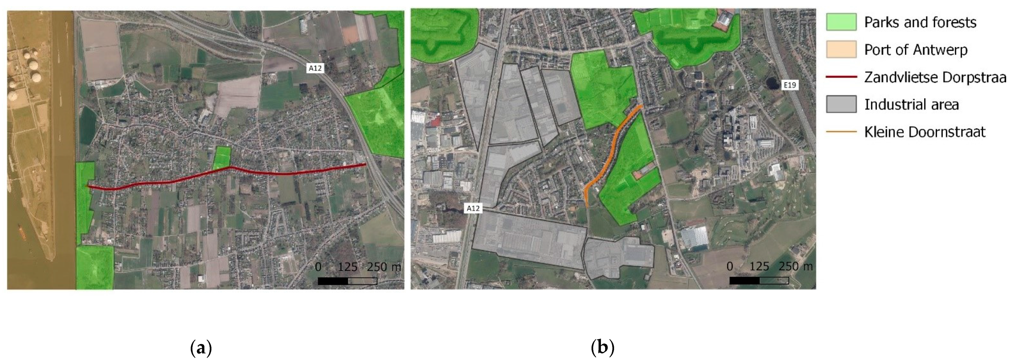
  • Location A: the average section length was 158 m. A new base layer was laid was recommend by guidelines from the Flemish road administration (SB250), in asphalt type APO-B (Dmax 14 mm), with 6 cm thickness, over a foundation composed of crushed stone. As a wearing course, three sections were laid in commercially available TALs, with 3 cm thickness, and two reference sections were built in SMA, with 10 and 6.3 mm maximum aggregate size and 4 cm thickness.
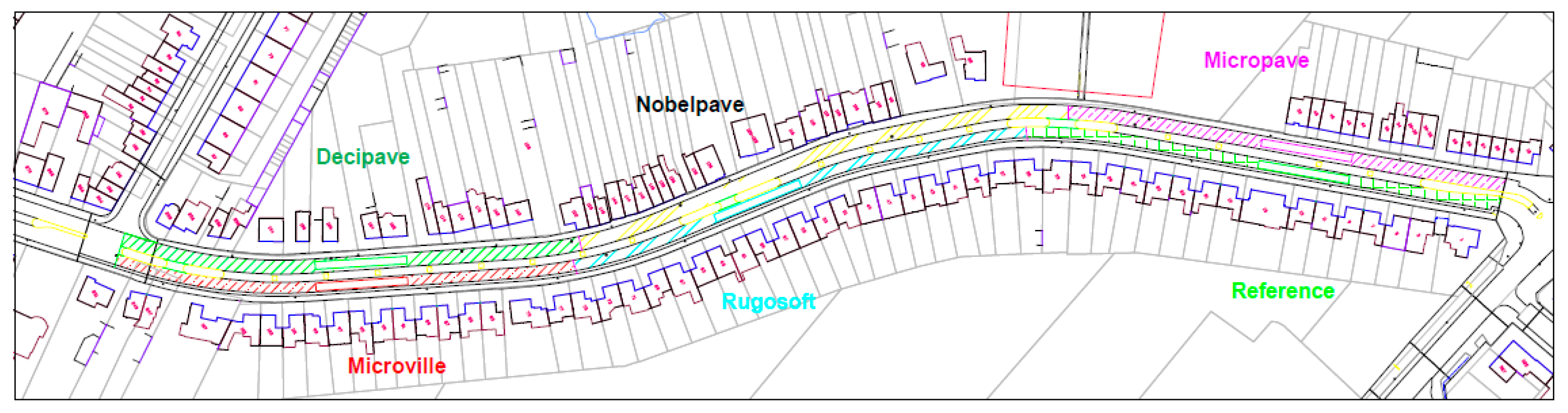
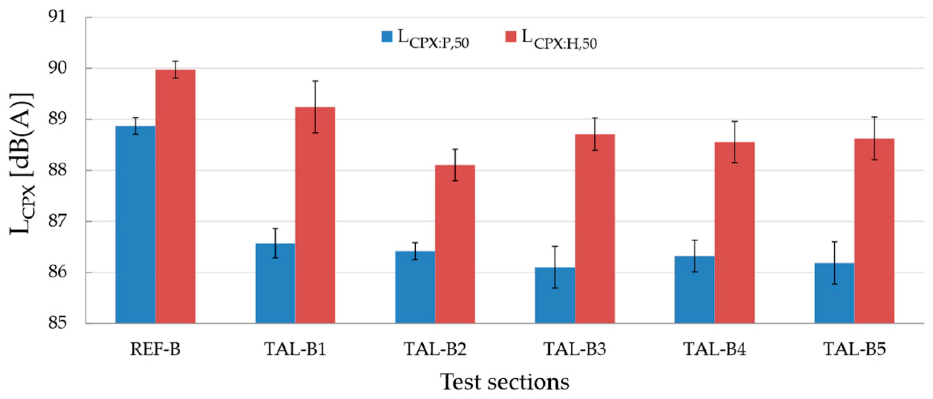
  • Location B: the sections presented an average length of 211 m. The foundation of crushed stone had approximately 28 cm thickness. Only part of the original base layer (type APO-B, Dmax 14 mm and 6 cm thickness) was replaced in order to reduce the costs and to obtain a different pavement than in location A. The existing wearing course (Dense Asphalt Concrete 0/10), laid 3 years before the TALs installation, was kept as a reference section (REF-B) due to its good condition. For the TALs construction, the wearing course was milled in 3 cm: the exact TALs thickness. Besides the three types of TALs used at location A, location B included two more sections in two different commercial TALs. The TAL sections at location B are hereafter named TAL-B1, TAL-B2, TAL-B3, TAL-B4 and TAL-B5. These TAL mixtures had maximum aggregate sizes of 5.8 to 6.3 mm and void contents ranging between 10 and 21%, classified as porous or semi-porous. Figure 2 presents the sections in location B, with the TALs’ commercial names. These were unrelated to the section numbering due to the anonymization agreements with the contractors.

2.1.2. Control Group

A group of streets where no noise intervention took place were chosen to serve as a control group. These streets were selected based on their residential comparability to the TAL streets (building typology and middle-class residents) and relatively quiet location. Ideally, the noise annoyance levels in these streets should be similar to those reported in local large scale surveys, in this case, the Survey on the Living Environment (Schriftelijk Leefomgevings Onderzoek—SLO), conducted in 2018 in the Flemish region, accounting for more than 5000 respondents [42]. Other requirements were local traffic with a speed restriction of 50 km/h, asphalt as pavement surface, similar building types, distance from highways, motorways, industry, airports, railways, etc. After several iterations and on-the-spot observations, five streets were selected across Antwerp: Tijl Uilenspiegellaan (Linkeroever), Verenigde Natieslaan (South-Antwerp), De Beuckelaerlaan, Ter Rivierenlaan and Schepersveldlei (North Antwerp). For the purpose of this study, the survey results from these streets were pooled and treated as a single group.

2.2. CPX and SPB Measurements

The acoustic performance of the sections was determined via SPB and CPX measurements. The CPX method aids in objectively determining the noise reduction and homogeneity of the sections. These measurements were performed by the Flemish Road Agency (Agentschap Wegen en Verkeer—AWV) 6 months after the works were concluded, as described in the standard ISO 11819-2 [40]. In this test, the tire/road noise was measured by driving over the pavement surface, at a reference speed of 50 km/h, with a trailer equipped with two sets of two microphones mounted close to the tire/road contact and enclosed into acoustically isolated chambers. Following ISO/TS 11819-3 [43], the Standard Reference Test Tire (SRTT-P1) and an Avon AV4 (H1) were used, representatives for car and truck tires, respectively. The noise levels (LCPX) and averaged third-octave band spectrum were obtained for individual 20 m sections. Due to a large number of parked cars at location A, CPX measurements were only performed at location B.
The SPB method is a roadside measurement used to determine the maximum sound pressure level and respective speed of passing-by vehicles from the normal fleet. The data are processed via regression analysis, and the average maximum sound pressure level for the dataset (Lveh) is calculated at a reference speed (50 km/h in this study) and per vehicle category. The results were adjusted by a correction coefficient of −0.10 dB(A)/°C, according to a semi-generic approach for dense road surfaces and at a reference temperature of 20 °C, as suggested in [44]. The measurements were conducted in location B 6 months after the TAL placement; the backing board was used to eliminate the possible influence from acoustic reflections, as required in ISO 11819-1 [41]. In location A, the distance of 7.5 m from the microphone to the center of the test lane could not be achieved in any spot of the street, impeding the SPB test to be conducted. CPX differs from the SPB method in accounting only for the tire/road noise and no other vehicle noise sources or propagation effects between the vehicle and the roadside. Therefore, SPB may represent better the actual noise exposure of residents living close-by the road [45].

2.3. Noise Modelling

Noise maps and noise exposure levels per façade (Lden and Lnight) were calculated using the CNOSSOS-EU calculation method implemented in the IMMI software [46]. This method requires certain inputs. Firstly, the terrain topography was obtained from the Digital Terrain Model Flanders II [47], created by the Flemish Agency for Geographical Information Flanders (AGIV), and imported to IMMI as contour lines that were converted into a terrain grid with 2 m resolution. For the calculation of the ground absorption, information was retrieved from three databases: a geographical database (Grootschalig Referentie Bestand), created by AGIV; one containing information on agricultural use (Landbouwgebruikspercelen), from the Agency for Agriculture and Fisheries; and a forest database (Digitale Boswijzer), constructed by the Agency for Nature and Forests. Building heights were determined using the 3D GRB database [48] and, due to the lack of databases, attributed a constant absorption coefficient of 0.2, as suggested by [39]. Additionally, CNOSSOS-EU requires corrections to account for differences in the vehicle fleet composition and weather among countries. For that, the adaptations created from the Dutch Standard Calculation Method 2 (SRM-2) to CNOSSOS-EU were employed [49].
Guidelines to determine the road surface correction terms, as presented in CNOSSOS-EU, often do not account for local or novel types of road surfaces. However, the Belgian Road Research Centre (BRRC) created a method to calculate these corrections using CPX results [45], which was employed in this study.
To model in IMMI, the higher-order reflections and distance between the source and image point (IP) also have to be set. These parameters were chosen to optimize calculation time without affecting the model’s accuracy, resulting in a limitation to third-order reflections and source-IP distances of 250 m for the first-order reflections and 500 m for the second and higher-order reflections.
Another required input for road traffic noise simulations is traffic volume. The Antwerp police department performed traffic counts in both road directions during three different timeframes: 6 months before and 1 and 6 months after the TALs installation. Each of these counts was taken during 24 h of 7 days in a row, as further detailed in Section 2.4.1. The traffic volume was further divided into the different traffic categories of CNOSSOS-EU, based on manual traffic counts.
The noise exposure and the noise maps were simulated using the original road surface as well as the surface after the TALs installation, taking into account the different sections. In order to compare the two conditions directly, all calculations were performed using the traffic count taken 6 months after the TAL installation. This timeframe was selected to match the CPX measurements. To avoid more variables except for the road surface type interfering with the noise exposure simulations between the two conditions, the CPX results obtained for the reference section (REF-B) were applied to the whole road surface in the original condition model. Noise maps were constructed using grid calculations. The average Lden and Lnight were obtained from façade levels calculations considering the external façade exposed to the highest Lden or Lnight per dwelling, as required by the END.

2.4. Self-Administered Surveys

Understanding the causal relations between objective noise, the perception of noise by exposed people and potential adverse health effects is essential for creating action plans for noise exposure mitigation [50]. The subjective impacts of the noise exposure in this work were evaluated via social surveys distributed to the residents of the control and experimental streets.

2.4.1. Content, Delivery and Response Rate

For locations A and B, two rounds of distribution of a written standardized survey to evaluate the impacts of the intervention on respondents’ noise perception were planned: firstly in April, 6 months before, and the second in November, 1 month after the TALs installation. However, the traffic counts conducted by the Antwerp police department showed considerably less traffic in location B during the time of the post-survey distribution than in the time of the pre-survey, as shown in Figure 3b. To avoid the reduction in traffic influencing road traffic noise and consequently the survey responses, a second post-survey was distributed at both locations in April of the following year, 6 months after the TAL installation.
In total, approximately 1200 envelopes were hand-delivered to the mailbox of each house in the streets studied. The envelope was marked with a sticker, including the University of Antwerp logo and a statement that a gift voucher would be raffled among those who replied before a given deadline, usually 4–6 weeks later. Besides the actual survey (six double-sided pages), the envelope contained a participation form for the gift voucher raffle, a prepaid return envelope, and a cover letter. The cover letter stated the purpose of the survey, the researchers involved, and the link for the survey’s online version. It was asked that only one respondent per house, above 18 years old, answered the survey; all respondents remained anonymous. The Ethics Committee for the Social Sciences and Humanities from the University of Antwerp approved the methodology and survey used.
The questionary comprised 27 questions, of which the first 10 were related to socio-demography. These questions were followed by five general questions taken from the SLO [42] regarding quality of life and annoyance. The annoyance-related questions assessed the overall annoyance level caused by different sources (noise, light, smell, and others) and noise annoyance caused by the different noise sources (air, rail and road traffic, priority vehicles, schools, etc.). The inclusion of different (noise) annoyance sources besides noise and road traffic aid to call the respondents’ attention to distinguish their overall (noise) annoyance from that caused by noise and road traffic noise specifically. The survey was further supplemented with additional in-depth questions regarding health problems, sleep quality, and the comfort level to perform certain activities indoors and outdoors.
We aimed to determine the subjective effectiveness of the traffic noise intervention based on the difference before and after the intervention of noise annoyance and health, sleep, and activity-related comfort while checking for the potential influence of differences in socio-demographics.
The following direct subjective noise indicators, referred to as “noise annoyance indicators”, were identified from the survey (see Figure 4). The verbal scale of the answers was formulated using a 5-point scale, as recommended by [11].
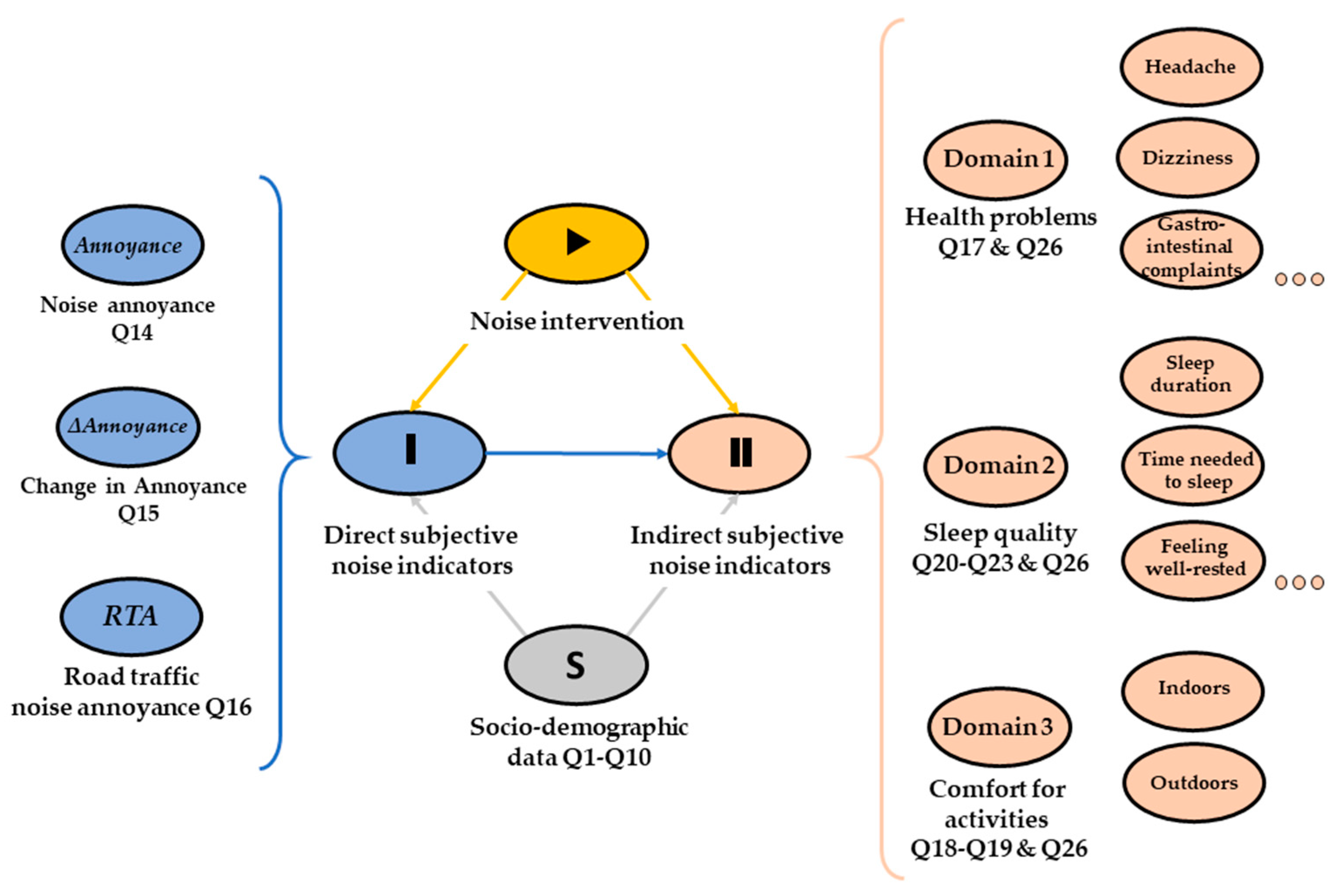
  • Annoyance: the extent of noise annoyance (all noise sources) in and around the house, perceived over the previous year, as formulated in Question 14_1: “Thinking about the last 12 months, to what extent were you annoyed by sound in and around your home?”. Response categories: Not at all (1), Slightly (2), Moderately (3), Very (4), and Extremely annoyed (5);
  • Change in annoyance (ΔAnnoyance): the reported change in Annoyance (all noise sources) over the previous two years, assessed in Question 15_1: “Thinking about your situation at home, in and around your house, to what extent has the annoyance caused by noise changed during the past 2 years?”. Response categories: Greatly reduced (−2), Slightly reduced (−1), Remained the same (0), Slightly increased (+1), and Greatly increased (+2);
  • Road traffic noise annoyance (RTA): the extent of annoyance caused specifically by road traffic noise, as formulated in Question 16_3: “To what extent are you annoyed by the following noise sources?”. Seven different noise sources were mentioned, including road traffic noise. Response categories: Not at all (1), Slightly (2), Moderately (3), Very (4), and Extremely annoyed (5);
The indirect subjective noise indicators were further investigated in three domains (see Figure 4):
  • Domain 1 (Physical complaints): the frequency respondents reported experiencing symptoms related to different health problems (headaches, fatigue, dizziness, insomnia, heart palpitations, and gastrointestinal complaints);
  • Domain 2 (Sleep quality): sleep duration and time needed to fall asleep, the frequency of feeling well-rested, waking up too early, or having difficulty waking up;
  • Domain 3 (Comfort level to perform activities): comfort level to conduct activities indoors and outdoors, as concentrating during working or studying, reading or watching television, speech intelligibility during a phone call or conversation, and relaxing or unwinding.
Figure 4 illustrates these indicators and the links checked among them considering the interference of the noise intervention, as further described in Section 2.4.2.
Table 2 presents the number of answers collected from the self-administered surveys. Response rates ranged from 18% to 35%. Locations with a relatively small population elicited a small number of answers as well, as in location A; thus, the limitations of the collected data must be considered.

2.4.2. Statistical Analysis

The direct and indirect subjective noise indicators were retrieved from 5-point scale answers and therefore considered ordinal variables. Due to the data type and the small group sizes, as presented in Table 2, nonparametric tests (Mann–Whitney U and Kruskal–Wallis tests) were performed to check for differences between the cases and conditions, at a 5% level significance [51,52]. Despite the ordinal nature of these variables, they were treated as continuous variables to calculate means and standard deviations. These measures of central tendency and variability create an illustrative comparability across contexts.
Profile characteristics differing among cases were identified via ANOVA or chi-square tests for continuous (as age) and binary variables (as gender), respectively. Additional analyses concerning possible links between these sociodemographic characteristics and the subjective noise indicators were carried out. In addition to demonstrating a link between the TAL construction and the noise annoyance indicators, the influence of noise annoyance on the three domains of the indirect subjective noise indicators was investigated using nonparametric Kendall τb correlations. This measure respects the measurement scales of the analyzed variables and has a similar interpretation as Pearson’s product-moment correlation coefficient r (even though the values of τb are usually lower than r). The τb gives insights on the strength and direction of associations between two ordinal variables: a value of ±1 indicates a perfect association between the two variables, whereas values close to 0 indicate weak or nonexistent relationships.

2.4.3. Sociodemographic Data

As the surveys were taken both before (pre) and two times after the TAL construction (post 1 and post 2), the same respondents could have answered the survey on more than one occasion. To analyze the sociodemographic profile, multiple respondents had to be removed from the dataset. As the answers were kept anonymous due to ethical constraints, these respondents were identified based on the match of six sociodemographic variables: street, gender, age, type of home, level of education, and the number of family members. If at least five of these six variables were the same between two different sets of surveys, it was ascribed as a double response and counted only once. Table 3 shows the most relevant part of the sociodemographic data of these unique respondents.
ANOVA tests with Tukey post-hoc analysis showed that the respondents in the reference streets were statistically significantly younger (p < 0.01) than the respondents in the streets where the TALs were placed. Concerning the level of education, more respondents in the streets in the control condition have obtained a master’s degree, either in a university college (two cycles: 4 or 5 academic years) or university. This is most likely explained by the tendency of younger people to pursue higher diplomas. The most commonly obtained qualification among the respondents for all streets was a bachelor’s degree (one cycle of 3 academic years). The percentage of respondents active in the labor market, the percentage of men and women, and respondents living with children did not differ significantly between the control and TAL streets. Further analysis of the possible influence of age and level of education on the subjective noise indicators is included in Section 4.3.

3. Effectiveness of the Noise Intervention

3.1. CPX and SPB Results

Figure 5 shows the LCPX for the experimental street B 6 months after the TALs construction, for both light (P) and heavy vehicles (H) at a reference speed of 50 km/h, calculated as the average of 20 m segments (included as the standard deviation).
All five TAL sections presented LCPX lower than the DAC 10 reference surface (REF-B). These differences ranged between 2.3 and 2.8 dB(A) for the P1 tire and 0.7 to 1.9 dB(A) for the H1 tire. For both tires, TAL-B1 presented the lowest noise reduction among the new surfaces. Furthermore, the standard deviation is the highest in this section, meaning a larger inhomogeneity between the 20 m segments.
The one-third octave band spectra were registered and served as input for the road corrections to calculate noise exposure. Even though the reductions in LCPX between the TALs and REF-B with H1 tire are less pronounced than with P1 tire, the traffic in location B mainly consisted of passenger cars, as it is an urban street. Therefore, the larger decreases in LCPX obtained with the P1 tire play a major role in the noise exposure calculation.
Table 4 shows the SPB results obtained only for passenger cars. The noise reductions ranging between 3.8 and 5.2 dB(A) should be significant enough for the residents close to the road to perceive the difference after the TALs construction.
Compared to the noise level reductions obtained with the CPX method, those measured with the SPB method are more pronounced. Most likely, the noise-absorbing characteristic of the (semi-) porous TALs is better captured in the SPB through the noise propagation path rather than the CPX, where the microphones are placed very close to the tire/road contact surface.

3.2. Noise Exposure and Noise Maps

The noise exposure results of the most exposed façade per dwelling in location B are shown as boxplots in Figure 6a (Lden) and Figure 6b (Lnight).
In the original condition, the residents were exposed to an average Lden of 64.3 ± 0.9 dB(A) and 53.8 ± 1.1 dB(A) for Lnight. After the TALs were laid, the average Lden dropped to 61.5 ± 0.8 dB(A), while Lnight was reduced to 51.0 ± 0.9 dB(A). Thus, the TALs placement led to a reduction of 2.8 dB(A) in both indicators.
The World Health Organization (WHO) updated in 2018 their environmental noise guidelines [54], strongly recommending public policies to limit road traffic noise levels to 53 dB(A) and 45 dB(A) for Lden and Lnight, respectively. These limits were not reached in the original condition, nor was the TAL placement capable of reducing the noise exposure to meet the recommended levels. Noise exposure levels were also calculated as grids. The difference grids, resulting from the subtraction of the before and after TAL maps, are shown in Figure 7.
The average drop of 2.8 dB(A) in Lden and Lnight calculated by the façade exposure is visible in Figure 7, as the houses in the vicinity of the road are mostly falling within the 2.5–3 dB(A) contour level. In the most northern part of the experimental street, where the reference section was kept, a reduction in noise exposure is still observed, resulting from the proximity to the low-noise sections. However, this reduction is distinguishably smaller than around the TALs sections.
As the TAL mixes are semi-porous or porous, their absorption coefficient is expected to be higher than the dense mixture (REF-B). However, as mentioned in Section 3.1., the CPX method does not properly account for this increased absorption. As the road corrections were calculated using the CPX results, it is expected that the noise exposure levels in the model with TALs are overestimated, resulting in a smaller decrease in Lden and Lnight compared to the original condition.

4. Effectiveness of the Noise Intervention

This section discusses the effects associated with reducing noise exposure levels enabled by the TALs placement. These impacts are expected to be reflected in the respondent’s perceptions within the social survey results.

4.1. Direct Subjective Perceived Noise: Annoyance Indicators

To assess the impacts of the TAL implementation on the annoyance indicators, we pooled the data from the two experimental streets (TAL A and TAL B) after finding no statistically relevant difference for the annoyance indicators of the pre-survey via the Mann–Whitney U test. Consequently, differences in the annoyance indicators after the intervention can be attributed to the TAL construction itself, not to differences between the two experimental cases.
The average and standard deviation of the annoyance indicators are presented in Table 5. The mean ranks’ differences among the conditions were tested with Kruskal–Wallis tests with Dunn’s post-hoc pairwise tests and significance levels were adjusted by the Bonferroni correction for multiple tests (see Table 6).
The main results to be found in Table 5 and Table 6 are the following:
  • The average Annoyance in the control streets (2.23 ± 0.99) indicates that respondents are ‘slightly annoyed’, compared to an average of 2.75 ± 1.11 (close to ‘moderately annoyed’) in pre-survey on the experimental streets. A similar condition is reported for RTA. For both indicators, the mean ranks difference is statistically significant. This contrast partially justifies the implementation of a noise intervention;
  • After the TAL construction, the ΔAnnoyance scores reveal that the residents experienced a lesser increase in annoyance by noise over the 1-year window prior to the post-surveys than before the pre-survey. Therefore, the residents report positively experiencing a change in Annoyance and RTA, most likely attributed to the noise intervention;
  • In the first post-survey, Annoyance and RTA have decreased in comparison to the pre-survey and are no longer significantly different from the control groups, where the average noise annoyance is close to the Flemish average reported in SLO-4 [42] (Annoyance = 2.11 and RTA = 2.19; based on >5000 respondents). This effect appears to be sustained even at the time of the second post-survey;
  • The three noise indicators did not differ statistically between post 1 and post 2. Thus, the lower traffic intensity might not be as influential on the reported subjective indicators as we anticipated, at least not in the short term;
  • Similar means for Annoyance and RTA across all cases possibly indicate that either the respondents did not differentiate between the noise sources causing annoyance or road traffic noise is clearly identified as the main source of Annoyance in general. The last option is more reasonable, as RTA is distinguishably the highest among the annoyances from the different noise sources: the second higher reported mean annoyance comes from ‘priority vehicles (ambulances, fire trucks, etc.)’, ranging from 1.64 to 1.78 across the three cases.
The percentage of highly annoyed people (%HA) is used to correlate annoyance to Lden, via ERRs. The %HA corresponds to the answers at a high position on the annoyance response scale. The cut-off point between “highly annoyed” and “not highly annoyed” differs among studies. Two often-cited ERRs for road traffic noise created based on large datasets are those of Guski et al. [4] and Miedema and Oudshoorn [6]. For the first, the cut-off lies at 75% on a 0–100 scale, meaning those who selected the 25% higher part of the response scale compose the %HA; for [6], this is at 72%.
To adapt this study’s verbal 5-point response scale to the most common definitions of %HA found in the literature, two cut-offs were used: 60% (very and extremely annoyed respondents) and 80% (extremely annoyed only). Additionally, the %HA was calculated using the simulated Lden as input for the ERRs proposed by Refs. [4,6] (in this case, the data set excluding the Alpine and Asian studies). The results are presented in Table 7.
The %HA (60%) dropped on average 15.2 percentage points (pp) from the pre-survey (26.8%) to the post-surveys (10–13.1%), resulting in a value smaller than the control streets (15.5%) and similar to the SLO-4 data (12.0%). %HA (80%) presents the same tendency but with smaller reductions (4.8 pp on average) due to the stricter cut-off. For the 2.8 Lden drop, these reductions are considerably more significant than those observed by [55], where 11.4% fewer people were highly annoyed by road traffic noise in streets presenting noise levels of LA,eq,24h < 55 dB(A) than in streets where these levels were higher than 65 dB(A).
Considering the differences in the cut-off, it can be argued that the ERRs by [4,6] are fairly reasonable in predicting the %HA with the Lden from before the TALs installation. The Lden after the TALs implementation led to calculated %HA higher than those obtained from the surveys, meaning that the actual drop in %HA due to the reduction in Lden is higher than the existing ERRs could predict. It is important to remark that the Lden calculated as per the CNOSSOS-EU method after the TALs implementation did not account for the increased absorption of these surfaces layers, resulting in a reduction of Lden smaller than it actually might have been. However, even if we recalculate the %HA with a Lden 1.5 dB(A) lower than simulated after the TALs implementation in an attempt to compensate for the underestimation, the ERRs still give a %HA higher than measured with the surveys.
Surveys organized in Copenhagen (2870 answers) on the annoyance levels before and after repaving two major roads with noise-reducing TAL, accounted for 10% fewer persons highly annoyed (at a 70% cut-off) after the TAL installation [35], as the result of a 4 dB Lden reduction (calculated per the Nord2000 calculation method). Dose–response curves constructed for both situations revealed that the respondents reacted to the noise levels they were exposed to, regardless of whether it was before or after the repaving. However, by comparing our measured %HA with the calculated, it does seem that the TAL implementation made the noise exposure–%HA relation more tilted. As noise annoyance is a subjective indicator that relies on the individual’s state of mind, the measured decrease in %HA may be attributed to an increased satisfaction regarding investments placed in infrastructure to enhance the resident’s quality of life. Additionally, the construction of TALs reduces noise levels without impacting, for example, the traffic flow or the environment aesthetics.

4.2. Indirect Subjective Perceived Noise: Physical Complaints, Quality of Sleep and Comfort Level to Perform Activities

The respondents indicated to what extent they were suffering from physical symptoms (Domain 1), sleeping quality (Domain 2), and difficulties performing activities indoors and outdoors (Domain 3). Kruskal–Wallis tests revealed no significant differences among the mean ranks of any indirect subjective indicator in three domains, neither for the different cases (control and experimental streets) nor conditions (pre- and post-surveys). Therefore, a direct link between the TAL implementation and the indirect subjective perceived noise could not be drawn. Ref. [50] stated that assessing potential health effects triggered by noise exposure should be mediated by annoyance indicators or other appraisal measures. This observation is also made in previous studies summarized in [27], all citing insufficient evidence to show direct links between noise interventions and sleep disturbance or cardiovascular effects.
Specifically for our research, we think three possible explanations can be given for the insignificant correlation between these indicators and the noise intervention. Firstly, the post-surveys might have been distributed too shortly after the intervention to find a measurable (health) effect. Physical complaints resulting from prolonged exposure to environmental noise will not immediately disappear after the noise levels have decreased. Secondly, the noise exposure reduction was limited (in the order of 3 dB). The third explanation is the sample size being insufficient to measure a reduction in complaints in the given research design.
Nonparametric Kendall’s τb correlation was used to determine whether there is a correlation between noise annoyance indicators and physical complaints, quality of sleep and comfort level to perform activities (Table 8). For that, the answers from the control streets and the pre-survey in the experimental streets were merged (recall that the two post-surveys are likely to present a significant number of double respondents and should not be included in computing correlations).
A large number of the indirect subjective noise indicators correlate weakly but significantly with the three annoyance indicators. In general, except for headaches, people who experience annoyance from (road traffic) noise are more likely to report physical complaints than people who are not. The perceived change ΔAnnoyance does not show correlation across Domain 1. In ref. [50], RTA is also related to fatigue, but not to chest pain.
The questionnaire data from a population-based study in Oslo [56] points out an association between road traffic noise and waking up too early. The present study further indicates that besides the actual noise levels, the noise annoyance indicators (Annoyance and RTA) may also aid in assessing this discomfort. Increasing levels of noise annoyance go with a lower likelihood of feeling well-rested in the morning. The other indicators in Domain 2 did not correlate significantly with the noise annoyances.
The strongest correlations in Table 8 were found in Domain 3. Without exception, it is more difficult to perform these activities when feeling annoyed by noise in general and specifically from road traffic (with the only exception of speaking to the phone). In general, the correlations were slightly stronger for outdoor activities. In the surveys conducted by [57], where 48.4% of the respondents reported experiencing noise-related annoyance (via a yes/no question), 49.8% reported feeling noise-induced discomfort to perform activities such as watching television, resting, talking and performing activities that require concentration.
Except for some of the correlations for comfort to perform outdoor activities, the τb values are generally low, which means that annoyance levels are contributing but certainly are not the only factor playing a role in the extent to which the respondents experience their sleeping pattern, physical complaints, or how comfortable they are to perform certain activities.

4.3. The Influence of Sociodemographics on Direct/Indirect Subjective Noise Indicators

As indicated in Section 2.4.3, only the variables age and level of education differ between the control and the experimental streets. Thus, only the impact of these two sociodemographic factors on the direct/indirect subjective noise indicators was further investigated. Nonparametric Kendall’s τb demonstrated that age did not correlate significantly with any of the annoyance indicators. The extent to which one has experienced (road traffic) annoyance or a change in annoyance did not vary with educational level. As the indirect subjective perceived noise indicators are not statistically different across cases, differences before and after intervention and between streets cannot be attributed to age or education. Therefore, the influence of age and education level becomes irrelevant for this discussion. These findings are in line with [50], who did not use sociodemographic modifying factors in their work as an exploratory multivariate analysis showed no interference of those in the annoyance indicators.

5. Summary and Conclusions

This study aimed to quantify the effectiveness of low-noise thin surface layers (TALs) as an intervention on road traffic noise and its impacts on the residents’ perception. Objectively, a noise exposure reduction of 2.8 dB(A) for both Lden and Lnight was obtained. However, the change in absorption coefficient due to the (semi-) porous characteristic of the TAL was not fully taken into account in the noise modelling, as the road correction terms of CNOSSOS-EU adopted in this study rely on CPX measurements. This observation is endorsed by the fact that the SPB results presented a higher decrease (up to 5.2 dB) in Lveh due to the TALs construction; as a roadside measurement method, SPB is more accurate in determining changes in road traffic noise in the propagation path than the CPX method. The noise exposure after the TALs placement still could not meet the recommended levels by the WHO [54] (Lden 61.5 dB and Lnight 51.0 dB compared to the limits of 53 dB and 45 dB, respectively). However, this is where the subjective impacts of the noise intervention become relevant, as the literature suggests that the impact of noise exposure on the build-up of non-auditory health disorders can be better assessed by the annoyance indicators rather than the actual noise levels.
Firstly, both the annoyance levels caused by noise in general and specifically by road traffic noise were significantly reduced after the TALs placement. These levels no longer differed from the levels reported in the control streets. The percentage of highly annoyed people (%HA) was reduced by 15.2% and 4.8%, for the cut-offs between highly annoyed and not highly annoyed at 60% and 80%, respectively. These reductions are considerably higher than based upon calculations using exposure–response relationships (ERRs) found in the literature ([4,6]). Considering the drop in Lden of 2.8 dB(A), the decrease in %HA measured in the surveys is more significant than the reduction observed in a large-scale study with TALs [7] as a noise intervention, where a 4 dB Lden drop led to 10% fewer persons highly annoyed (at a 70% cut-off). Perhaps the residents’ satisfaction was increased by the implementation of a policy to enhance their well-being. Additionally, an advantage of TALs to enable road traffic noise reductions is the absence of negative impacts such as interference on the environment aesthetics, as noise barriers do, or a change in traffic flow as brought by implementing stricter speed limits.
The indirect subjective noise indicators, which included physical complaints, sleep quality, and comfort level to perform activities indoors or outdoors, did not present a change after the noise intervention. This result may be attributed to the fact that health outcomes caused by noise exposure are better perceived in the long-term, while the surveys were taken shortly after the TALs implementation. Small sample size and limited reduction in Lden may also have played a role in obscuring/hiding possible changes. Annoyance and RTA presented a weak but statistically significant correlation with several physical complaints. We also found that residents who are more annoyed by (road traffic) noise reported an increased difficulty to perform most of the activities listed in the surveys, both outdoors and indoors. Regarding sleeping quality, however, almost no significant correlations were found with the noise annoyance indicators. The explanation may be that neutral sounds, as from road traffic noise, do not disturb the sleep as much as loud noise events [58], especially when the nocturnal traffic volume is much smaller than during the day, as shown in Figure 3 (average pass-by vehicles at night are 8 to 15 times lower than during the day). Thus, the annoyance levels reported by the respondents are majorly related to their perception of noise during the daytime. While these findings on sleep quality perhaps contradict previous findings, those studies confirming a noise annoyance–sleep disturbance relation [57,58] phrase the questions on sleep problems in terms of noise (e.g., “to what degree is your sleep disturbed when you are at home from sound from road noise?”), which was deliberately not implemented in our study to avoid measuring artefacts. Even though the sociodemographic profile of the residents showed that age and education level differed from the experimental to the control streets, we found no evidence that these characteristics had an impact on the annoyance levels.
The results from this study support the policies of (road) authorities in general and in cities such as Antwerp in particular, to continue investing in projects that reduce road traffic noise annoyance, provided that sufficient residents in the region can benefit from the intervention and that it is technically feasible.

6. Limitations and Outlook

A limitation of this study was the low number of respondents (174 in the control streets, 57 and 86 in pre- and post-surveys, respectively, in the experimental streets), partly attributed to the difficulty of finding suitable and feasible sites to implement the TALs in the urban environment, especially due to lack of political support. With a low number of respondents, local and individual effects can play an amplified role in the average indirect perceived noise, e.g., work schedules, time spent at home, noise sensitivity and acoustical façade insulation. Therefore, in scenarios where a noise intervention such as TALs are placed, more large-scale studies are still needed to comprehend the relations between changes in objective noise levels and its subjective perception by the exposed population. By doing so, steady-state ERRs could fairly estimate the annoyance levels, reducing the costs and time invested in conducting social surveys.
Besides Lden and Lnight, other potential predictors could be relevant for the annoyance estimation, such as the intermittent character of the noise source, exposure to other transportation noise sources, and temperature. Lastly, the noise exposure reduction due to the TALs obtained in this study was relatively low. We expect that in situations with a higher initial noise exposure followed by a more significant decrease due to the noise intervention, as in the vicinity of highways where noise barriers are installed, the effects of the intervention are more pronounced. This is the object of study of upcoming works of the authors.

Author Contributions

Conceptualization, A.G.d.B., J.K.K. and C.V.; Formal analysis, A.G.d.B. and J.K.K.; Funding acquisition, C.V.; Investigation, J.K.K. and C.V.; Methodology, J.K.K. and C.V.; Project administration, C.V.; Supervision, C.V.; Visualization, A.G.d.B., J.K.K. and C.V.; Writing—original draft, A.G.d.B., J.K.K. and C.V.; Writing—review and editing, A.G.d.B., J.K.K. and C.V. All authors have read and agreed to the published version of the manuscript.

Funding

This research was partly funded by the City of Antwerp through the research project with acronym STOLA—Stille TOpLagen voor Antwerpen, and by the University Research Fund at the University of Antwerp through the project BOF/KP/39652.

Institutional Review Board Statement

The study was conducted according to the guidelines of the Declaration of Helsinki, and approved by the Institutional Review Board (or Ethics Committee) of the University of Antwerp (protocol code: SHW_16_22, date of approval: 8 August 2016).

Informed Consent Statement

Informed consent was obtained from all subjects involved in the study.

Data Availability Statement

The data presented in this study are available on request from the corresponding author. The data are not publicly available due to privacy issues.

Acknowledgments

The authors would like to thank, first of all, the anonymous participants in the surveys. Secondly, we are grateful to the City of Antwerp and the Flemish Agency for Roads and Traffic (AWV) for their assistance in this research (funding, measurement data, access to additional information, …). Next, the authors would like to thank all people involved in the STOLA-project and the master students who helped to gather all relevant measurement and survey data. Among the master’s students, we thank Arnout Breens in particular for constructing the initial version of the noise maps and bringing up relevant discussions to the content of this paper. Last but not least, we are grateful to Sarah De Roeck for her extensive English review as a native speaker.

Conflicts of Interest

The authors declare no conflict of interest. The funders had no role in the design of the study; in the collection, analyses, or interpretation of data; in the writing of the manuscript, or in the decision to publish the results.

References

  1. Hänninen, O.; Knol, A.B.; Jantunen, M.; Lim, T.-A.; Conrad, A.; Rappolder, M.; Carrer, P.; Fanetti, A.-C.; Kim, R.; Buekers, J.; et al. Environmental Burden of Disease in Europe: Assessing Nine Risk Factors in Six Countries. Environ. Health Perspect. 2014, 122, 439–446. [Google Scholar] [CrossRef] [Green Version]
  2. Ögren, M.; Molnár, P.; Barregard, L. Road traffic noise abatement scenarios in Gothenburg 2015–2035. Environ. Res. 2018, 164, 516–521. [Google Scholar] [CrossRef] [PubMed]
  3. Basner, M.; Babisch, W.; Davis, A.; Brink, M.; Clark, C.; Janssen, S.; Stansfeld, S. Auditory and non-auditory effects of noise on health. Lancet 2014, 383, 1325–1332. [Google Scholar] [CrossRef] [Green Version]
  4. Guski, R.; Schreckenberg, D.; Schuemer, R. WHO Environmental Noise Guidelines for the European Region: A Systematic Review on Environmental Noise and Annoyance. Int. J. Environ. Res. Public Health 2017, 14, 1539. [Google Scholar] [CrossRef] [PubMed] [Green Version]
  5. Brink, M.; Schäffer, B.; Vienneau, D.; Foraster, M.; Pieren, R.; Eze, I.C.; Cajochen, C.; Probst-Hensch, N.; Röösli, M.; Wunderli, J.-M. A survey on exposure-response relationships for road, rail, and aircraft noise annoyance: Differences between continuous and intermittent noise. Environ. Int. 2019, 125, 277–290. [Google Scholar] [CrossRef] [PubMed]
  6. Miedema, H.M.E.; Oudshoorn, C.G. Annoyance from transportation noise: Relationships with exposure metrics DNL and DENL and their confidence intervals. Environ. Health Perspect. 2001, 109, 409–416. [Google Scholar] [CrossRef] [PubMed]
  7. Hong, J.; Lee, S.; Lim, C.; Kim, J.; Kim, K.; Kim, G. Community annoyance toward transportation noise: Review of a 4-year comprehensive survey in Korea. Appl. Acoust. 2018, 139, 229–234. [Google Scholar] [CrossRef]
  8. Ascigil-Dincer, M.; Demirkaleb, S. Model development for traffic noise annoyance prediction. Appl. Acoust. 2021, 177, 229–234. [Google Scholar] [CrossRef]
  9. Asutay, E.; Västfjäll, D. Perception of loudness is influenced by emotion. PLoS ONE 2012, 7, e38660. [Google Scholar] [CrossRef] [Green Version]
  10. Crichton, F.; Dodd, G.; Schmid, G.; Petrie, K.J. Framing sound: Using expectations to reduce environmental noise annoyance. Environ. Res. 2015, 142, 609–614. [Google Scholar] [CrossRef] [PubMed]
  11. Fields, J.M. Effect of personal and situational variables on noise annoyance in residential areas. J. Acoust. Soc. Am. 1993, 93, 2753–2763. [Google Scholar] [CrossRef]
  12. Miedema, H.M.E.; Vos, H. Demographic and attitudinal factors that modify annoyance from transportation noise. J. Acoust. Soc. Am. 1999, 105, 3336–3344. [Google Scholar] [CrossRef]
  13. Pershagen, G.; Van Kempen, E.; Casas, M.; Foraster, M. Traffic noise and ischemic heart disease—Review of the evidence for the WHO environmental noise guidelines for the European region. Eur. Heart J. 2017, 38, 710. [Google Scholar] [CrossRef] [Green Version]
  14. E Beutel, M.; Brähler, E.; Ernst, M.; Klein, E.; Reiner, I.; Wiltink, J.; Michal, M.; Wild, P.S.; Schulz, A.; Münzel, T.; et al. Noise annoyance predicts symptoms of depression, anxiety and sleep disturbance 5 years later. Findings from the Gutenberg Health Study. Eur. J. Public Health 2020, 30, 487–492. [Google Scholar] [CrossRef] [PubMed]
  15. Okokon, E.O.; Yli-Tuomi, T.; Turunen, A.W.; Tiittanen, P.; Juutilainen, J.; Lanki, T. Traffic noise, noise annoyance and psychotropic medication use. Environ. Int. 2018, 119, 287–294. [Google Scholar] [CrossRef]
  16. Bodin, T.; Björk, J.; Ardö, J.; Albin, M. Annoyance, Sleep and Concentration Problems due to Combined Traffic Noise and the Benefit of Quiet Side. Int. J. Environ. Res. Public Health 2015, 12, 1612–1628. [Google Scholar] [CrossRef] [PubMed]
  17. Wang, H.; Gao, H.; Cai, M. Simulation of traffic noise both indoors and outdoors based on an integrated geometric acoustics method. Build. Environ. 2019, 160, 106201. [Google Scholar] [CrossRef]
  18. Stansfels, S.; Clark, C. Health Effects of Noise Exposure in Children. Curr. Environ. Health Rep. 2015, 2, 171–178. [Google Scholar] [CrossRef] [PubMed] [Green Version]
  19. Babisch, W.; Beule, B.; Schust, M.; Kersten, N.; Ising, H. Traffic Noise and Risk of Myocardial Infarction. Epidemiology 2005, 16, 33–40. [Google Scholar] [CrossRef]
  20. Petri, D.; Licitra, G.; Vigotti, M.A.; Fredianelli, L. Effects of Exposure to Road, Railway, Airport and Recreational Noise on Blood Pressure and Hypertension. Int. J. Environ. Res. Public Health 2021, 18, 9145. [Google Scholar] [CrossRef]
  21. Dratva, J.; Phuleria, H.C.; Foraster, M.; Gaspoz, J.-M.; Keidel, D.; Künzli, N.; Liu, L.-J.S.; Pons, M.; Zemp, E.; Gerbase, M.W.; et al. Transportation Noise and Blood Pressure in a Population-Based Sample of Adults. Environ. Health Perspect. 2012, 120, 50–55. [Google Scholar] [CrossRef] [PubMed]
  22. European Parliament, Council of the European Union. Assessment and management of environmental noise. In Directive 2002/49/EC of the European Parliament and of the Council of 25 June 2002; 32002L0049; European Commission: Brussels, Belgium, 2002. [Google Scholar]
  23. Felcyn, J.; Preis, A.; Kokowski, P.; Gałuszka, M. A comparison of noise mapping data and people’s assessment of annoyance: How can noise action plans be improved? Transp. Res. Part D Transp. Environ. 2018, 63, 72–120. [Google Scholar] [CrossRef]
  24. Directive, E. Commission Directive (EU) 2015/996 of 19 May 2015 Establishing Common Noise Assessment Methods according to Directive 2002/49/EC of the European Parliament and of the Council; 32015L0996R(01); European Commission: Brussels, Belgium, 2015. [Google Scholar]
  25. Murphy, E.; Faulkner, J.P.; Douglas, O. Current State-of-the-Art and New Directions in Strategic Environmental Noise Mapping. Curr. Pollut. Rep. 2020, 6, 54–64. [Google Scholar] [CrossRef]
  26. Nilsson, M.; Bengtsson, J.; Klaeboe, R. Environmental Methods for Transport Noise Reduction, 1st ed.; CRC Press: London, UK, 2014. [Google Scholar]
  27. Brown, A.L.; van Kamp, I. WHO Environmental Noise Guidelines for the European Region: A Systematic Review of Transport Noise Interventions and Their Impacts on Health. Int. J. Environ. Res. Public Health 2017, 14, 873. [Google Scholar] [CrossRef] [Green Version]
  28. Sandberg, U.; Ejsmont, J. Tyre/Road Noise Reference Book; Informex: Kisa, Sweden, 2002. [Google Scholar]
  29. Bianco, F.; Fredianelli, L.; Castro, F.L.; Gagliardi, P.; Fidecaro, F.; Licitra, G. Stabilization of a p-u Sensor Mounted on a Vehicle for Measuring the Acoustic Impedance of Road Surfaces. Sensors 2020, 20, 1239. [Google Scholar] [CrossRef] [Green Version]
  30. Gateano, L.; Mauro, C.; Elena, A. Noise monitoring within LIFE NEREiDE: Methods and results. In Proceedings of the Inter-Noise 2019: The 48th International Congress and Exhibition on Noise Control Engineering, Madrid, Spain, 16–19 June 2019. [Google Scholar]
  31. Del Pizzo, A.; Teti, L.; Moro, A.; Bianco, F.; Fredianelli, L.; Licitra, G. Influence of texture on tyre road noise spectra in rubberized pavements. Appl. Acoust. 2020, 159, 107080. [Google Scholar] [CrossRef]
  32. Biligri, K.P. Effect of pavement materials’ damping properties on tyre/road noise characteristics. Constr. Build. Mater. 2013, 49, 223–232. [Google Scholar] [CrossRef]
  33. Merskaa, O.; Mieczkowski, P.; Żymełkaa, D. Low-noise Thin Surface Course—Evaluation of the Effectiveness of Noise Reduction. Transp. Res. Procedia 2016, 14, 2688–2697. [Google Scholar] [CrossRef] [Green Version]
  34. Vaitkus, A.; Andriejauskas, T.; Vorobjovas, V.; Jagniatinskis, A.; Fiks, B.; Zofka, E. Asphalt wearing course optimization for road traffic noise reduction. Constr. Build. Mater. 2017, 152, 345–356. [Google Scholar] [CrossRef]
  35. Pedersen, T.H.; Le Ray, G.; Bendtsen, H.; Bendtsen, J. Community Response to Noise Reducing Road Pavements. Rapport Nr. 502; Danish Road Directorate (Vejdirektoratet): Copenhagen, Denmark, 2014.
  36. Lo Castro, F.; Iarossi, S.; Massimiliano, L.; Bernardini, M. Life NEREiDE project: Preliminary evaluation of road traffic noise after new pavement laying. In Proceedings of the Inter-Noise 2019: The 48th International Congress and Exhibition on Noise Control Engineering, Madrid, Spain, 16–19 June 2019. [Google Scholar]
  37. Torija, A.J.; Flindell, I.H. Listening laboratory study of low height roadside noise barrier performance compared against in-situ field data. Build. Environ. 2014, 81, 216–225. [Google Scholar] [CrossRef]
  38. Bergiers, A. Pilot study in Antwerp to study the acoustical quality and durability of thin noise reducing asphalt layers in an urban environment. In Proceedings of the Inter-Noise 2018: The 47th International Congress and Exposition on Noise Control Engineering, Chicago, IL, USA, 26–29 August 2018. [Google Scholar]
  39. Maeck, J.; Bergiers, A. Noise Reducing Thin Asphalt Layers in an Urban Environment: A pilot study in Antwerp. In Proceedings of the Inter-Noise 2016: The 45th International Congress and Exposition on Noise Control Engineering, Hamburg, Germany, 21–24 August 2016. [Google Scholar]
  40. EN ISO. Acoustics—Measurement of the Influence of Road Surfaces on Traffic Noise—Part 2: The Close-Proximity Method; EN ISO 11819-2:2017; The International Organization for Standardization: Geneva, Switzerland, 2017. [Google Scholar]
  41. EN ISO. Acoustics—Measurement of the Influence of Road Surfaces on Traffic Noise—Part 1: Statistical Pass-By Method; EN ISO 11819-1:1997; The International Organization for Standardization: Geneva, Switzerland, 1997. [Google Scholar]
  42. Environment Department. Schriftelijk Leefomgevingsonderzoek SLO-4 (2018). Available online: https://www.lne.be/schriftelijk-leefomgevingsonderzoek-slo-4-2018 (accessed on 29 September 2021). (In Dutch).
  43. EN ISO/TS. Acoustics—Measurement of the Influence of Road Surfaces on Traffic Noise—Part 3: Reference Tyres; EN ISO/TS 11819-3:2017; The International Organization for Standardization: Geneva, Switzerland, 2017. [Google Scholar]
  44. Bühlmann, E.; van Blokland, G. Temperature effects on tyre/road-noise—A review of empirical research. In Proceedings of the Forum Acusticum 2014, Kraków, Poland, 7–12 September 2014. [Google Scholar]
  45. Ledee, F.A.; Goubert, L. The determination of road surface corrections for CNOSSOS-EU model for the emission of road traffic noise. In Proceedings of the 23rd International Congress on Acoustics, Aachen, Germany, 9–13 September 2019. [Google Scholar]
  46. Wölfel. IMMI [Computer Software]. Available online: https://www.immi.eu/en/ (accessed on 29 September 2021).
  47. AGIV. Digitaal Hoogtemodel Vlaanderen II, DTM, Raster, 1 m, Brussel. Available online: https://download.vlaanderen.be/Producten/Detail?id=939&title=Digitaal_Hoogtemodel_Vlaanderen_II_DTM_raster_1_m (accessed on 29 September 2021).
  48. AGIV. 3D GRB, 2019. Available online: https://download.vlaanderen.be/Producten/Detail?id=971&title=3D_GRB (accessed on 21 August 2021).
  49. Wesseling, J.; van Velze, K. Technische Beschrijving van Standaardrekenmethode 2 (SRM-2) voor Luchtkwaliteitsberekeningen; RIVM Briefrapport 2014-0109; The Dutch National Institute for Public Health and the Environment: Utrecht, The Netherlands, 2015.
  50. Fyhri, A.; Klæboe, R. Road traffic noise, sensitivity, annoyance and self-reported health—A structural equation model exercise. Environ. Int. 2009, 35, 91–97. [Google Scholar] [CrossRef] [PubMed]
  51. Lehman, E.L. Nonparametrics: Statistical Methods Based on Ranks, 2nd ed.; Springer: New York, NY, USA, 2006. [Google Scholar]
  52. De Winter, J.; Dodou, D. Five-Point Likert Items: t test versus Mann-Whitney-Wilcoxon. Pract. Assess. Res. Eval. 2010, 15, 147–151. [Google Scholar]
  53. Vuye, C.; Fraeyman, J.; Kampen, J.K.; Musovic, F.; Tyszka, L.; Van den bergh, W.; Beeckman, R.; Van Dessel, A.; Bergiers, A.; Maeck, J.; et al. The impact of thin noise reducing asphalt layers on the quality of life in an urban environment. In Proceedings of the EuroRegio2016, Porto, Portugal, 13–15 June 2016. [Google Scholar]
  54. WHO. Environmental Noise Guideline for the European Region; WHO: Copenhagen, Denmark, 2018. [Google Scholar]
  55. Paunovic, K.; Jakovljević, B.; Belojevic, G. Predictors of noise annoyance in noisy and quiet urban streets. Sci. Total. Environ. 2009, 407, 3707–3711. [Google Scholar] [CrossRef]
  56. Evandt, M.J.; Oftedal, B.; Krog, N.H.; Nafstad, P.; Schwarze, P.E.; Aasvang, G.M. A Population-Based Study on Nighttime Road Traffic Noise and Insomnia. Sleep 2016, 40. [Google Scholar] [CrossRef] [PubMed]
  57. Paiva, K.M.; Cardoso, M.R.A.; Zannin, P.H. Exposure to road traffic noise: Annoyance, perception and associated factors among Brazil’s adult population. Sci. Total Environ. 2019, 650, 978–986. [Google Scholar] [CrossRef]
  58. Berg, F.V.D.; Verhagen, C.; Uitenbroek, D. The Relation between Scores on Noise Annoyance and Noise Disturbed Sleep in a Public Health Survey. Int. J. Environ. Res. Public Health 2014, 11, 2314–2327. [Google Scholar] [CrossRef] [PubMed] [Green Version]
Figure 1. Orthophotomap in scale 1:30,000. (a) location A (Zandvlietse Dorpstraat); (b) location B (Kleine Doornstraat).
Sustainability 13 12561 g001
Figure 2. Test tracks installed at location B.
Sustainability 13 12561 g002
Figure 3. TAL streets: traffic counts taken at the time of the surveys over 1 week. (a) location A; (b) location B (two driving directions). * Due to a technical malfunction, only 1 day could be measured.
Sustainability 13 12561 g003
Figure 4. Indicators and correlations retrieved from the surveys.
Sustainability 13 12561 g004
Figure 5. CPX results from location B for the different test sections (measurement data from AWV).
Sustainability 13 12561 g005
Figure 6. Noise exposure presented as boxplots with average, median, quartiles, and internal points. (a) Lden; (b) Lnight.
Sustainability 13 12561 g006
Figure 7. Difference grids, resulting from the subtraction of the before and after TAL noise maps (simulated in IMMI). (a) Lden; (b) Lnight.
Sustainability 13 12561 g007
Table 1. Information on the streets equipped with TAL.
LocationStreet NameBuilding
Typology
Traffic
Intensity
Heavy TrafficOther Noise Sources
AZandvlietse Dorpstraatdetached and semi-detachedvery lowno
(only local traffic)
A12 highway (2 km)
Railway (2 km)
Port of Antwerp (2 km)
BKleine Doornstraatterraced and semi-detachedaverageyesA12 and E19 highway (<1 km)
Antwerp airport (5 km)
Industrial area (<1 km)
Table 2. Number of respondents per location and case.
Noise
Intervention
Region/LocationNumber of Respondents
ControlPrePost 1Post 2TotalResp. Rate
---North Antwerp
Linkeroever
South Antwerp
Subtotal
93
32
49
174
-
-
-
-
-
-
-
-
-
-
-
-
93
32
49
174
28%
35%
18%
25%
TALA
B
Subtotal
-
-
-
19
38
57
12
34
46
14
26
40
45
98
143
20%
35%
28%
Total 17457464031726%
Table 3. Sociodemographic data of the unique respondents.
IndicatorControlTAL
Sex
Women
Men

46.7%
53.3%

52.1%
47.9%
Age39.2 ± 16.255.9 ± 15.4
Level of education *
Low
Middle
High

11.8%
51.6%
36.6%

17.1%
53.8%
26.4%
Inactive ×39.7%46.9%
Living with children33.3%42.7%
* Level of education was registered in eleven categories, but reduced to three for this analysis: low (no schooling completed, primary school and general/technical/vocational lower secondary school), middle (general/technical/vocational upper secondary school and bachelor’s degree—one cycle of 3 academic years), and high (master’s degree at a university college—two cycles: 4 or 5 academic years—or university). × We categorized all retired and unemployed people (whether or not looking for a job) as inactive. All others (including students) are categorized as active.
Table 4. SPB test results for location B (based on data from [53]).
SectionSPB (@ 50 km/h) [dB(A)]Reduction [dB(A)]
REF-B71.0---
TAL-B167.23.8
TAL-B266.24.8
TAL-B367.23.8
TAL-B467.13.9
TAL-B565.85.2
Table 5. Average annoyance indicators (standard deviation).
IndicatorCase
ControlTAL
PrePost 1Post 2
Annoyance *2.23 (0.99)2.75 (1.11)2.48 (1.01)2.42 (0.75)
ΔAnnoyance ×0.46 (0.85)0.87 (0.79)0.16 (1.07)0.00 (1.22)
RTA *2.29 (1.08)2.86 (1.10)2.51 (0.92)2.41 (0.99)
* Response scale: Not annoyed at all = 1; Slightly annoyed = 2; Moderately annoyed = 3; Very annoyed = 4; Extremely annoyed = 5. × Response scale: Greatly reduced = −2; Slightly reduced = −1; Remained the same = 0; Slightly increased = 1; Greatly increased = 2.
Table 6. Pairwise multiple comparisons results for the noise annoyance indicators.
ContrastAnnoyanceΔAnnoyanceRTA
p-Value
ControlPre<0.010.02<0.01
Post 1n.s.n.s.n.s.
Post 2n.s.n.s.n.s.
PrePost1n.s.<0.01n.s.
Post2n.s.<0.01n.s.
Post 1Post 2n.s.n.s.n.s.
χ2(3) = 12.62, p = 0.006χ2(3) = 19.17, p = 0.000χ2(3) = 4.17, p = 0.006
n.s. = not significant at a 5% significance level.
Table 7. Measured and calculated %HA with existing ERRs.
Measured %HACalculated %HA
80%60%[4] 75%[6] 72%
Control streets2.515.5..
TALPre7.126.817.515.2
Post 12.213.113.211.8
Post 22.510.0
Reduction pre to post (average)4.815.24.33.4
Table 8. Kendall’s τb correlations between indirect subjective perceived noise and annoyance indicators.
DomainIndicatorAnnoyanceΔAnnoyanceRTA
Physical complaints (1)Headaches
Fatigue0.14 * (n = 220) 0.13 * (n = 211)
Dizziness0. 0.15 * (n = 210)
Insomnia0.22 ** (n = 224) 0.16 ** (n = 214)
Heart palpitations0.14 * (n = 221) 0.15 * (n = 213)
Gastrointestinal complaints0.13 * (n = 223) 0.12 * (n = 215)
Sleep quality (2)Sleep duration (night)
Sleep duration (day) −0.13 * (n = 212)
Time to fall asleep
Waking up too early0.15 ** (n = 221) 0.14 * (n = 213)
Difficulty waking up
Feeling well-rested−0.14 * (n = 220)
Comfort level to perform activities (3)Concentration during readingIn0.21 ** (n = 223) 0.20 ** (n = 214)
Out0.56 ** (n = 222)0.16 ** (n = 209)0.20 ** (n = 213)
Concentration during working or studyingIn0.22 ** (n = 218) 0.13 * (n = 210)
Out0.31 ** (n = 218)0.13 * (n = 205)0.18 ** (n = 208)
Concentration during watching TVIn0.18 ** (n = 223) 0.14 * (n = 213)
Speech intelligibility during a conversationIn0.20 ** (n = 221) 0.12 * (n = 213)
Out0.30 ** (n = 223)0.24 ** (n = 210)0.26 ** (n = 213)
Speech intelligibility on the telephoneIn0.18 ** (n = 224)0.15 * (n = 211)
Out0.29 ** (n = 222)0.21 **(n = 209)0.22 ** (n = 212)
Relaxing or unwindingIn0.23 ** (n = 223)0.17 ** (n = 210)0.16 ** (n = 214)
Out0.38 ** (n = 222)0.26 ** (n = 209)0.24 ** (n = 213)
* Correlation is significant at the 0.05 level (2-tailed). ** Correlation is significant at the 0.01 level (2-tailed).
Publisher’s Note: MDPI stays neutral with regard to jurisdictional claims in published maps and institutional affiliations.

