
Return Rate Prediction in Blockchain Financial Products Using Deep Learning


Abstract
:1. Introduction
- Design a new return rate predictive model using RRP-DLBFP for blockchain financial product
- Develop an LSTM model for the predictive analysis of return rate
- Propose an Adam optimizer to adjust the hyperparameters of the LSTM model optimally
- Design an OGSO algorithm for the optimal adjustment of learning rate in the LSTM model
- Validate the performance of the RRP-DLBFP technique under several aspects
2. Related Work
3. Methodology
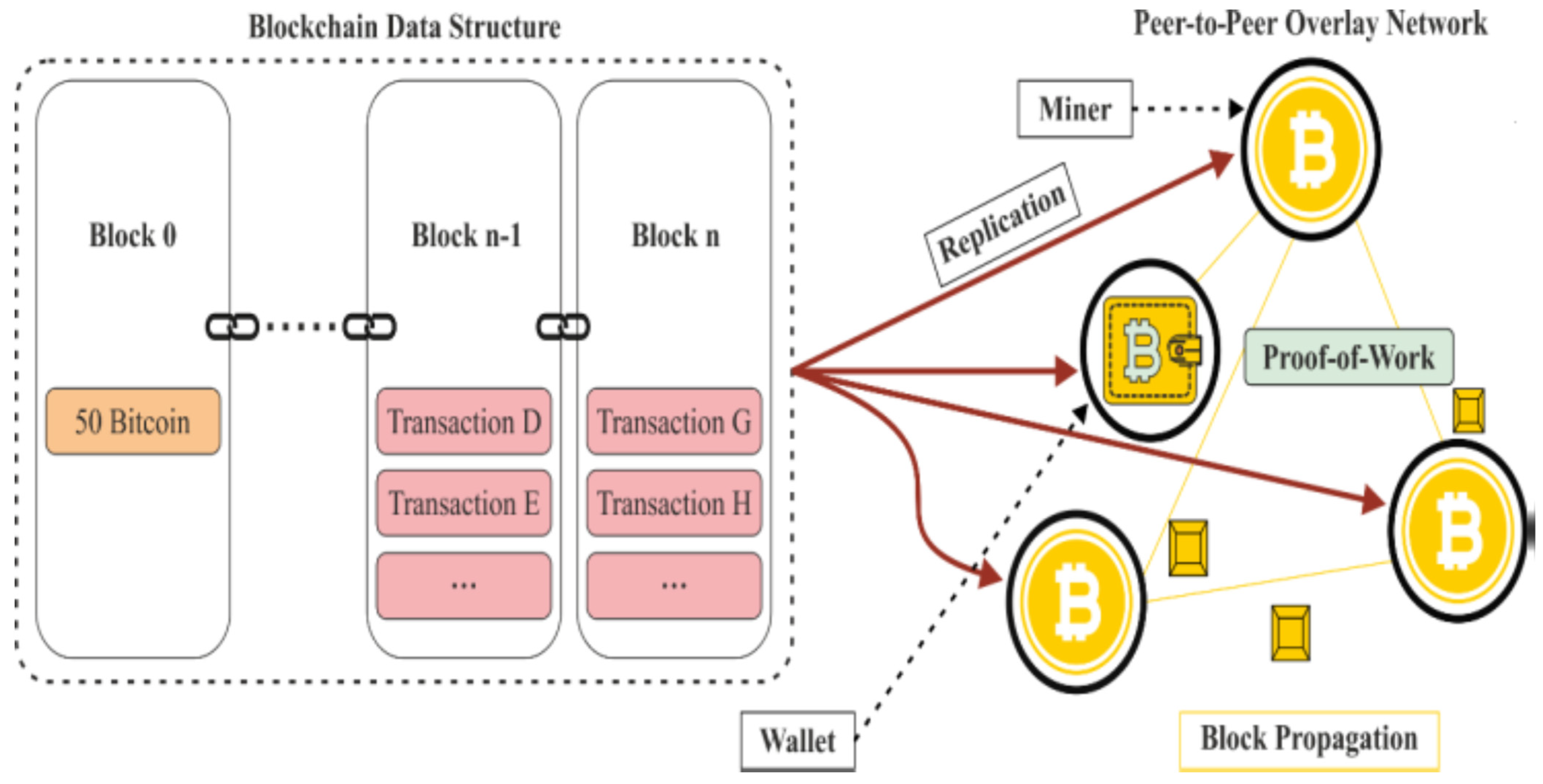
3.1. Blockchain
3.2. LSTM
3.3. Adam Optimizer
| Algorithm 1. The proposed method for optimizing the LSTM model’s parameters. The elementwise square is represented by . Default machine learning settings that are effective so far include and when working with vectors, you must always do things element by element. With and we denote and to the power . |
| Inout: sizeOfstep, : Stochastic objective function uses parameters : Estimates with exponential decay rate for the instant, = Initial vector (initial value of moment vector) (initial value of second moment vector) (initial timestep) |
Output , (Return parameters )
|
4. The Proposed RRP-DLBFP Model Design
- Fluorescence in concentration
- Neighboring set
- Decision domain radius
- Moving possibility
- Glowworm location
5. Experimental Validation
6. Conclusions
Author Contributions
Funding
Institutional Review Board Statement
Informed Consent Statement
Data Availability Statement
Conflicts of Interest
References
- Saadah, S.; Whafa, A.A. Monitoring Financial Stability Based on Prediction of Cryptocurrencies Price Using Intelligent Algorithm. In Proceedings of the 2020 International Conference on Data Science and Its Applications (ICoDSA), Bandung, Indonesia, 5–6 August 2020; pp. 1–10. [Google Scholar]
- Subramanian, H. Decentralized blockchain-based electronic marketplaces. Commun. ACM 2017, 61, 78–84. [Google Scholar] [CrossRef]
- Yilmaz, N.K.; Hazar, H.B. Predicting future cryptocurrency investment trends by conjoint analysis. J. Econ. Financ. Account. 2018, 5, 321–330. [Google Scholar] [CrossRef]
- Lee, R.S. Time series chaotic neural oscillatory networks for financial prediction. In Quantum Finance; Springer: Singapore, 2020; pp. 301–337. [Google Scholar]
- Lee, R.S. Chaotic interval type-2 fuzzy neuro-oscillatory network (CIT2-FNON) for Worldwide 129 financial products prediction. Int. J. Fuzzy Syst. 2019, 21, 2223–2244. [Google Scholar] [CrossRef]
- Sigova, M.V.; Klioutchnikov, I.K.; Zatevakhina, A.V.; Klioutchnikov, O.I. Approaches to evaluating the function of prediction of decentralized applications. In Proceedings of the 2018 International Conference on Artificial Intelligence Applications and Innovations (IC-AIAI), Nicosia, Cyprus, 31 October–2 November 2018; pp. 1–6. [Google Scholar]
- Schlegel, M.; Zavolokina, L.; Schwabe, G. Blockchain technologies from the consumers’ perspective: What is there and why should who care? In Proceedings of the 51st Hawaii International Conference on System Sciences, Hilton Waikoloa Village, HI, USA, 3–6 January 2018. [Google Scholar]
- Saracevic, M.; Wang, N.; Zukorlic, E.E.; Becirovic, S. New Model of Sustainable Supply Chain Finance Based on Blockchain Technology. Am. J. Bus. Oper. Res. 2021, 3, 61–76. [Google Scholar] [CrossRef]
- Salah, K.; Rehman, M.H.; Nizamuddin, N.; Al-Fuqaha, A. Blockchain for AI: Review and open research challenges. IEEE Access 2017, 7, 10127–10149. [Google Scholar] [CrossRef]
- Fischer, T.; Krauss, C. Deep learning with long short-term memory networks for financial market predictions. Eur. J. Oper. Res. 2018, 270, 654–669. [Google Scholar] [CrossRef] [Green Version]
- Zhang, Z. Improved adam optimizer for deep neural networks. In Proceedings of the 2018 IEEE/ACM 26th International Symposium on Quality of Service (IWQoS), Banff, AB, Canada, 4–6 June 2018; pp. 1–2. [Google Scholar]
- Kiktenko, E.O.; Pozhar, N.O.; Anufriev, M.N.; Trushechkin, A.S.; Yunusov, R.R.; Kurochkin, Y.V.; Lvovsky, A.I.; Fedorov, A.K. Quantum-secured blockchain. Quantum Sci. Technol. 2018, 3, 035004. [Google Scholar] [CrossRef] [Green Version]
- Hussein, A.F.; ArunKumar, N.; Ramirez-Gonzalez, G.; Abdulhay, E.; Tavares, J.M.; de Albuquerque, V.H. A medical records managing and securing Blockchain based system supported by a genetic algorithm and discrete wavelet transform. Cogn. Syst. Res. 2018, 52, 1–11. [Google Scholar] [CrossRef] [Green Version]
- Huang, W.; Nakamori, Y.; Wang, S.Y. Forecasting stock market movement direction with support vector machine. Comput. Oper. Res. 2005, 32, 2513–2522. [Google Scholar] [CrossRef]
- Indera, N.I.; Yassin, I.M.; Zabidi, A.; Rizman, Z.I. Non-linear autoregressive with exogeneous input (NARX) Bitcoin price prediction model using PSO-optimized parameters and moving average technical indicators. J. Fundam. Appl. Sci. 2017, 9, 791–808. [Google Scholar] [CrossRef]
- Kaur, S.; Singh, K.D.; Singh, P.; Kaur, R. Ensemble Model to Predict Credit Card Fraud Detection Using Random Forest and Generative Adversarial Networks. In Emerging Technologies in Data Mining and Information Security; Springer: Singapore, 2021; pp. 87–97. [Google Scholar]
- Poongodi, M.; Sharma, A.; Vijayakumar, V.; Bhardwaj, V.; Sharma, A.P.; Iqbal, R.; Kumar, R. Prediction of the price of Ethereum blockchain cryptocurrency in an industrial finance system. Comput. Electr. Eng. 2020, 81, 106527. [Google Scholar]
- Sivaram, M.; Lydia, E.L.; Pustokhina, I.V.; Pustokhin, D.A.; Elhoseny, M.; Joshi, G.P.; Shankar, K. An optimal least square support vector machine based earnings prediction of blockchain financial products. IEEE Access 2020, 8, 120321–120330. [Google Scholar] [CrossRef]
- Celeste, V.; Corbet, S.; Gurdgiev, C. Fractal dynamics and wavelet analysis: Deep volatility and return properties of Bitcoin, Ethereum and Ripple. Q. Rev. Econ. Financ. 2020, 76, 310–324. [Google Scholar] [CrossRef]
- Sifat, I.M.; Mohamad, A.; Shariff, M.S. Lead-lag relationship between bitcoin and ethereum: Evidence from hourly and daily data. Res. Int. Bus. Financ. 2019, 50, 306–321. [Google Scholar] [CrossRef]
- Shah, D.; Zhang, K. Bayesian regression and Bitcoin. In Proceedings of the 2014 52nd Annual Allerton Conference on Communication, Control, and Computing (Allerton), Monticello, IL, USA, 30 September–3 October 2014; pp. 409–414. [Google Scholar]
- Matta, M.; Lunesu, I.; Marchesi, M. Bitcoin Spread Prediction Using Social and Web Search Media. In Proceedings of the UMAP Workshops, 23rd Conference on User Modeling, Adaptation and Personalization, Dublin, Ireland, 29 June–3 July 2015; pp. 1–10. [Google Scholar]
- Matta, M.; Lunesu, I.; Marchesi, M. The predictor impact of Web search media on Bitcoin trading volumes. In Proceedings of the 2015 7th International Joint Conference on Knowledge Discovery, Knowledge Engineering and Knowledge Management (IC3K), Lisbon, Portugal, 12–14 November 2015; Volume 1, pp. 620–626. [Google Scholar]
- Gu, B.; Konana, P.; Liu, A.; Rajagopalan, B.; Ghosh, J. Identifying information in stock message boards and its implications for stock market efficiency. 2006. Available online: http://www.ideal.ece.utexas.edu/pdfs/151.pdf (accessed on 5 September 2021).
- Greaves, A.; Au, B. Using the bitcoin transaction graph to predict the price of bitcoin. Comput. Sci. 2015, 1–8. [Google Scholar]
- Madan, I.; Saluja, S.; Zhao, A. Automated Bitcoin Trading via Machine Learning Algorithms. Volume 20. 2015. Available online: http://cs229.stanford.edu/proj2014/Isaac%20Madan,%20Shaurya%20Saluja,%20Aojia%20Zhao,Automated%20Bitcoin%20Trading%20via%20Machine%20Learning%20Algorithms.pdf (accessed on 5 September 2021).
- Delfin-Vidal, R.; Romero-Meléndez, G. The fractal nature of bitcoin: Evidence from wavelet power spectra. In Trends in Mathematical Economics; Pinto, A., Accinelli Gamba, E., Yannacopoulos, A., Hervés-Beloso, C., Eds.; Springer: Cham, Switzerland, 2016; pp. 73–98. [Google Scholar]
- Kristoufek, L. What are the main drivers of the Bitcoin price? Evidence from wavelet coherence analysis. PLoS ONE 2015, 10, e0123923. [Google Scholar] [CrossRef] [PubMed]
- White, H. Economic prediction using neural networks: The case of IBM daily stock returns. ICNN 1988, 2, 451–458. [Google Scholar]
- Koskela, T.; Lehtokangas, M.; Saarinen, J.; Kaski, K. Time series prediction with multilayer perceptron, FIR and Elman neural networks. In Proceedings of the World Congress on Neural Networks, Bochum, Germany, 16–19 July 1996; pp. 491–496. [Google Scholar]
- Giles, C.L.; Lawrence, S.; Tsoi, A.C. Noisy time series prediction using recurrent neural networks and grammatical inference. Mach. Learn. 2001, 44, 161–183. [Google Scholar] [CrossRef] [Green Version]
- Rather, A.M.; Agarwal, A.; Sastry, V.N. Recurrent neural network and a hybrid model for prediction of stock returns. Expert Syst. Appl. 2015, 42, 3234–3241. [Google Scholar] [CrossRef]
- McNally, S.; Roche, J.; Caton, S. Predicting the price of bitcoin using machine learning. In Proceedings of the 2018 26th Euromicro International Conference on Parallel, Distributed and Network-Based Processing (PDP), Cambridge, UK, 21–23 March 2018; pp. 339–343. [Google Scholar]
- Catanzaro, B.; Sundaram, N.; Keutzer, K. Fast support vector machine training and classification on graphics processors. In Proceedings of the Proceedings of the 25th International Conference on Machine Learning, Helsinki, Finland, 5–9 July 2008; pp. 104–111. [Google Scholar]
- Cireşan, D.C.; Meier, U.; Gambardella, L.M.; Schmidhuber, J. Deep, big, simple neural nets for handwritten digit recognition. Neural Comput. 2010, 22, 3207–3220. [Google Scholar] [CrossRef] [PubMed] [Green Version]
- Mehdizadeh, M. Integrating ABC analysis and rough set theory to control the inventories of distributor in the supply chain of auto spare parts. Comput. Ind. Eng. 2020, 139, 105673. [Google Scholar] [CrossRef]
- Liu, Y.; Zhang, Q.; Fan, Z.P.; You, T.H.; Wang, L.X. Maintenance spare parts demand forecasting for automobile 4S shop considering weather data. IEEE Trans. Fuzzy Syst. 2018, 27, 943–955. [Google Scholar] [CrossRef]
- Chang, Z.; Zhang, Y.; Chen, W. Electricity price prediction based on hybrid model of adam optimized LSTM neural network and wavelet transform. Energy 2019, 187, 115804. [Google Scholar] [CrossRef]
- Zheng, Z.; Xie, S.; Dai, H.N.; Chen, X.; Wang, H. Blockchain challenges and opportunities: A survey. Int. J. Web Grid Serv. 2018, 14, 352–375. [Google Scholar] [CrossRef]
- Li, X.; Jiang, P.; Chen, T.; Luo, X.; Wen, Q. A survey on the security of blockchain systems. Futur. Gener. Comput. Syst. 2020, 107, 841–853. [Google Scholar] [CrossRef] [Green Version]
- Zhao, Z.; Chen, W.; Wu, X.; Chen, P.C.; Liu, J. LSTM network: A deep learning approach for short-term traffic forecast. IET Intell. Transp. Syst. 2017, 11, 68–75. [Google Scholar] [CrossRef] [Green Version]
- Bello, I.; Zoph, B.; Vasudevan, V.; Le, Q.V. Neural optimizer search with reinforcement learning. In Proceedings of the 34th International Conference on Machine Learning, ICML 2017, Sydney, Australia, 6–11 August 2017; pp. 459–468. [Google Scholar]
- Jayakumar, D.N.; Venkatesh, P. Glowworm swarm optimization algorithm with topsis for solving multiple objective environmental economic dispatch problem. Appl. Soft Comput. 2014, 23, 375–386. [Google Scholar] [CrossRef]


| Models | Training Dataset | Testing Dataset | ||
|---|---|---|---|---|
| MSE | MAPE | MSE | MAPE | |
| RRP-DLBFP | 0.0435 | 2.9845 | 0.0655 | 3.9856 |
| GANMLP | 0.0698 | 3.1902 | 0.0962 | 4.2890 |
| PSOLSSVR | 0.0701 | 3.2126 | 0.0973 | 4.3531 |
| SVM | 0.1091 | 4.7237 | 0.1132 | 4.5721 |
| BPNN | 0.0712 | 3.2356 | 0.1021 | 4.7372 |
| GA-SVM | 0.0945 | 4.4697 | 0.1032 | 4.6938 |
| ANN | 0.0978 | 4.5860 | 0.1076 | 4.7139 |
| Random Walk | 0.1014 | 4.3146 | 0.1034 | 4.3154 |
Publisher’s Note: MDPI stays neutral with regard to jurisdictional claims in published maps and institutional affiliations. |
© 2021 by the authors. Licensee MDPI, Basel, Switzerland. This article is an open access article distributed under the terms and conditions of the Creative Commons Attribution (CC BY) license (https://creativecommons.org/licenses/by/4.0/).
Share and Cite
Metawa, N.; Alghamdi, M.I.; El-Hasnony, I.M.; Elhoseny, M. Return Rate Prediction in Blockchain Financial Products Using Deep Learning. Sustainability 2021, 13, 11901. https://doi.org/10.3390/su132111901
Metawa N, Alghamdi MI, El-Hasnony IM, Elhoseny M. Return Rate Prediction in Blockchain Financial Products Using Deep Learning. Sustainability. 2021; 13(21):11901. https://doi.org/10.3390/su132111901
Chicago/Turabian StyleMetawa, Noura, Mohamemd I. Alghamdi, Ibrahim M. El-Hasnony, and Mohamed Elhoseny. 2021. "Return Rate Prediction in Blockchain Financial Products Using Deep Learning" Sustainability 13, no. 21: 11901. https://doi.org/10.3390/su132111901
APA StyleMetawa, N., Alghamdi, M. I., El-Hasnony, I. M., & Elhoseny, M. (2021). Return Rate Prediction in Blockchain Financial Products Using Deep Learning. Sustainability, 13(21), 11901. https://doi.org/10.3390/su132111901