Analyzing Urban Public Policies of the City of Ensenada in Mexico Using an Attractive Land Footprint Agent-Based Model

Sandoval-Félix, Javier; Castañón-Puga, Manuel; Gaxiola-Pacheco, Carelia Guadalupe

doi:10.3390/su13020714

Open AccessArticle

Analyzing Urban Public Policies of the City of Ensenada in Mexico Using an Attractive Land Footprint Agent-Based Model

by

Javier Sandoval-Félix

^*,†,‡,

Manuel Castañón-Puga

^*,†,‡

and

Carelia Guadalupe Gaxiola-Pacheco

^†

Facultad de Ciencias Químicas e Ingeniería, Universidad Autónoma de Baja California, México 22390, Mexico

^*

Authors to whom correspondence should be addressed.

^†

Current Address: Calzada Universidad 14418, Tijuana, Baja California, México 22390, Mexico.

^‡

These authors contributed equally to this work.

Sustainability 2021, 13(2), 714; https://doi.org/10.3390/su13020714

Submission received: 30 November 2020 / Revised: 26 December 2020 / Accepted: 29 December 2020 / Published: 13 January 2021

(This article belongs to the Special Issue Sustainability Challenges in Real Estate Markets and Urban Property Developments)

Abstract

:

The Urban Development Plan of the city of Ensenada, México (UDPE) states four major strategic projects, one of which mandates to “Acquire and enable new land reserves and expand opportunities for economic and social development.” This is of vital importance given the large number of vacant lots that perforates the urban surface in contrast to the physical limitations of growth demarcated by hill areas of a steep slope, which forces a sustainable use of the land. These are important growth challenges, affecting aspects such as the real estate market, in particular, that related to industrial activities, which has not matured due to outdated planning practice, resulting in industrial sprawl. This paper shows an institutional effort to analyze the UDPE from a Complex Systems approach with an Agent-Based Model, adapting Peter Allen’s concept of Structural Attractor. This attraction results from an agglomeration of UDPE’s regulatory attributes and real estate investor’s land-acquisition criteria that affects the spatial behavior of vacant land that is attractive for industrial activity. Unlike physical land uses, these attractive zones emerge, grow, move, diminish, and emerge again over time in the form of Attractive Land Footprints. Understanding these phenomena is vital for local policymakers. The findings indicate that the current Urban Plan is ill-suited regarding current industry development expectations. The model also showed unexpected roles played by population density, road network, and residential land use in Attractive Land Footprint dynamics, acting as a thought-provoking process for policymakers and real estate investors, as it helped them to understand Ensenada’s industry phenomena.

Keywords:

attractive land footprints; land planning, urban public policies; agent-based modeling; multi-agent systems; social simulation

1. Introduction

A current characteristic of the city of Ensenada (The city of Ensenada is located in Mexico at the coordinates 31°51′28″ N 116°36′21″ W), México that has concerned both its municipal authorities and investors is the challenge of promoting and harmoniously integrating industrial activities into the urban land in the face of untapped opportunities and challenges that have gotten worse over time. Among these are industrial sprawl due to a lack of industrial land-use policy implementation and at the same time, an abundance of vacant lots that currently represent 10% of the urban surface. This has led to a gradual stagnation of the industrial real estate market and worsening of the population’s quality of life through land-use incompatibilities between adjacent industrial and residential areas, damage to streets not suitable for industrial traffic, long commute times, and street obstructions, among others. In a recent project called Sectoral Programme of Industrial Development of Ensenada [1] it is estimated that 48% of the industry is in normative incompatibility with the Urban Development Plan of Ensenada (UDPE) [2], 87% of the properties that host this activity are in lots less than one hectare contrary to the recommendation of 10 hectares [3] and 59% of this activity is on lower hierarchy streets. Together with Ensenada´s abrupt topography, it has resulted in having the lowest percentage of industrial land-use surface of all the state cities with 1.45% of the total urban area. Despite the current unfavorable spatial distribution of industrial activity, it is noteworthy that the city has had three iterations of its UDPE with clear regulations for the orderly distribution of land-uses. Still, the industry has not occupied the territory as planned, settling in areas stated as incompatible by these planning instruments. The city has already occupied the entire coastal plain, where it first developed, which is surrounded by steep slopes. Looking into the near future, the competition for vacant land will exacerbate at the detriment of activities that have not yet satisfied their demand for land. Considering this, having new planning approaches and public policies focused on efficient use of the finite urban land resources are crucial.

In 2018 the municipal government started updating its UDPE. Part of this exercise was to have a forecast of land use patterns to identify the most feasible areas of vacant land to cluster new industrial developments as a way to reduce industrial sprawl and have more efficient use of available lots. These scenarios would then be compared with current urban regulations to identify possible adjustment needs, as was the case with the UDPE’s Land-Use Compatibility Matrix (See supplementary file). This planning tool regulates where land uses can be carried out or what activities can be carried out in specific sectors of the city. It is composed of 111 land uses and 61 spatial subsectors (Figure 1), which in total yields 6771 compatibility decisions. And even though from a normative perspective the development of industrial activity is allowed, it is still necessary to integrate other environmental, social, or infrastructure factors that will weigh on the industrial real estate developer final decision to build a factory, such as the slope of the land, adjacent activities, proximity to labor, or connectivity with primary roads. Recognizing the complex nature of this process is that the municipal planning office decided to analyze the public policies of the UDPE from a complex systems approach, focusing on urban spatial patterns through an agent-based modeling methodology as is is estimated that it can bring insights relevant to policy design and land planning practice. Urban sprawl is a central matter for approaching sustainable living and production models due to its economic, social, and environmental outgrowths [4]. The objective was to develop a model that would help in the identification and analysis of emerging industry-attractive vacant land patterns as a result of the spatial agglomeration of favorable conditions for this use. Once these areas were obtained, called Attractive Land Footprints, they were compared with current UDPE regulations to assess probable updates.

Urban sprawl is a topic subject to debate among planners and researchers, who are still far from a consensual solution. If urban form emerges from multiple overlapping interactions between households, firms, and governmental bodies, we could approach urban spatial dynamics from the complex systems’ perspective. In [5] we can find a review of the sprawl debate from the complexity sciences. In the context of urban development, a significant challenge is to design better public policies in an environment of uncertainty and slow progress in urban knowledge, recognizing the city as a complex entity that emerges from the interaction of a large number of environmental, social, economic and institutional components. The approach described is the complex systems perspective. Complex systems can be defined as systems in which large networks of components without central control and simple rules of operation give rise to complex collective behavior [6]. Since it can be applied to phenomena where a large number of interacting components are present, it has been used for the study of seemingly dissimilar fields such as markets [7], epidemics [8], social networks [9], traffic [10], crowds [11], public policies [12] and cities [13]. In cities’ analysis, complexity has functioned as a complementary approach to several urban disciplines, providing a theoretical basis to study and understand a variety of urban phenomena and properties that were previously considered independent of each other and interpreted by different theoretical bases [14]. The conception of cities under the complex systems approach is called Complex Urban Systems, where population, economic growth, the increase in urbanization levels, the dependence on infrastructure and the role of technology in society are considered elements that drive urban complexity [15].

One aim of urban analysis from a complexity approach is to discover new ways of addressing urban challenges in a context of uncertainty, posing as an alternative to the traditional process of public policy design that is unaware of interactions with domains supposedly unrelated to the problem originally intended to address and that will operate in a highly complex space beyond what can be controlled or observed in a deterministic way [16]. It must provide knowledge about cities by identifying emerging behaviors and anticipating how they can be affected by the implementation of policies before their application in real life and identifying new relationships between urban structure and dynamics that allow more successful solutions. Thus, through computational simulation, besides forecasting, explaining and controlling [17], the planning activity would have relevant conceptual implications for those who design and implement public policies [18].

The spatial rise, displacement, diminishment and rise again of Attractive Land Footprints (Figure 2) relates to one of the most distinct aspect of complex systems: emergence. Defined as the rise of new and coherent structures, properties and patterns during the process of self-organization [19], it relates in turn to pattern formation, a topical area of complex systems.

This paper is related to the emergence of urban spatial patterns, but unlike the characteristics normally associated with land uses, which are physical, visible, and immovable; the patterns studied here are an agglomeration of attributes that together make a vacant land attractive for certain land uses, specifically for this study, industrial activities. These attributes emerge, move, disappear, and emerge again in other places responding to urban regulations, territorial factors, and real estate investor’s land-acquisition criteria. For this paper, they are called Attractive Land Footprints (Figure 2), similar to a concept applied to systems by Peter Allen called Structural Attractor, which he defines as “… the emergence of a set of interacting factors that have mutually supportive, complementary attributes.” [14].

Although he used this concept to refer to the behavior of a system and not to any component of it, the definition itself describes admirably well the concept of Attractive Land Footprints for the context of this research. The idea that an area is attractive has been used as a context in numerous papers that pursue other ultimate research goals, or even in gravitational urban models [20] but not under the characteristics of the complex behavior of Attractive Land Footprints. Even so, the interacting factors referred to by Allen can be considered to make an area attractive for a land use. These factors can be employment and services [20,21], land cost, physical risk, coastal zones [7,22,23,24], travel time [20,25], productivity [26], proximity to urban centers, accessibility to transportation systems [27,28], urbanization and existing land uses [29,30], housing [31], infrastructure [32], availability of building land, income level [33], current occupancy status [20], population density, water price [34], elevation, flood zones, proximity to commercial areas, proximity to water, industrial density [35], light industry [36], distance to urban sub-centers, proximity to railways and rivers [37], total saleable areas [38], green areas, climate, lakes and scenic views [39,40,41,42], agricultural areas and large open spaces [43], garbage dumps [30], urban peripheries [44], schools and hospitals [45], sports facilities [24], topography and zoning [46]. Depending on the number, combination and arrangement of these factors in the territory, it will be the land use that tends to attract (Table A1 in Appendix A.1).

We organized this paper as follows. Firstly, we presented the methodology, where we introduced the concept of Attractive Land Footprint and the computational modeling process (We simulated Ensenada City Attractive Land Footprint by using a spatial model of cellular automata developed in the NetLogo programming environment). Then, in the next section, we presented the simulation results analysis and discussion. We make some conclusions according to the findings, and we suggest future work.

2. Methodology

The methodology is of an exploratory nature whose objective is to have numerous urban pattern scenarios as an aid to decision making and policy design, specifically about vacant land that is attractive for industrial activities. The concept of Attractive Land Footprint is introduced, which is simulated through a spatial model of cellular automata developed in the Netlogo programming environment and described through the ODD protocol (Overview, Design Concepts, Details) [47] in Appendix C.

It follows a process similar to the one presented by [48], which starts with the system analysis, followed by the conceptual modeling of the system, design of the simulation, generation of the code for the simulation, preparation of the simulation, execution of the simulation and ends with the analysis of the results (Figure A1 in Appendix B). The methodology is broken down in greater detail in Appendix B.

2.1. Data Requirements

For this methodology’s application, two main components are needed:

(1): Spatial data layers. For this current exercise, the layers were composed of the city´s polygon boundaries, sub-sectors boundaries, urban grid, water bodies, terrain slope, agricultural zones, developed land, non-developable land, developable land, road structure, and current land uses. They should be in SHP or ASC format, depending on the case (Table A2 in Appendix B).
(2): Urban development plan regulations applicable to the human settlement to be modeled. The spatial data layers and the Urban Development Plan (Table A3 in Appendix B) must belong to the same time cut. For this exercise, the Land Use Compatibility Matrix was used as the regulatory norm to be evaluated.

2.2. Model Verification and Validation

The information referred to in the previous sections is the basis for hypothesis verification, which is done through a cellular automaton model. The model is used to execute a series of experiments, for which the following must be done beforehand:

2.2.1. Model Verification

The model’s internal consistency should be checked, verifying that all the functionalities are executed according to expected results, according to the following criteria:

(1): Developable land. Land uses should only grow on developable land and in previously established slope ranges.
(2): Compatibility matrix. According to the subsector where they are located, the land uses that grow on the territory are only those allowed by the compatibility matrix.
(3): Adjacency matrix. Adjacent land uses must be those that are only permitted by an adjacency matrix.
(4): Population projection. The current and projected population for each year should be the same. This comparison will be made with ex-ante scenarios, that is, with previously known results.
(5): Urban surface. The amount of urban surface generated each year should correspond to population projection and density established at the beginning of the model’s execution.

2.2.2. Model Validation

A face value comparison is made between simulated and real-world urban growth patterns. The variable that controls the degree of urban sprawl is called Threshold, which is explained in the ODD protocol.

2.2.3. Sample Space

The number of iterations that each experiment must be executed will be determined by a face-value approximation analysis to the sample space, that is, the set of all possible outcomes under the same set of initial variables.

2.3. Experiments

The experiments are exploratory and results are focused on analyzing the behaviour of industry-attractive vacant land spatial patterns as a result of the agglomeration of existing land uses, urban regulations, and real estate investor’s land-acquisition criteria (Figure 3). The model outputs are relevant to this sector, and municipal authorities, such as the availability, location, and occupancy competition of vacant land by land uses other than industry, emergent spatial patterns, and compliance with the urban regulations of the UDPE. The model will be executed a number of times equal to the sample space previously identified, under real-world variables of population number, growth rate, and density per hectare. All the simulations will have the same growth projection of ten years. NetLogo’s BehaviorSpace tool allows the same model to be run a specific number of times with pre-established parameters. The results are classified by item in CSV format (comma-separated value). These experiments, their output and usefulness to the real estate market and public authorities are stated in Table 1.

Additionally, the simulations are executed with a population density of 10, 15, 20, 25, 30, 35, 40, 45, 50, 55, 60, 65, 70, 75, 80, 85, 90, 95 and 100 inhabitants per hectare and variability in percentage compliance to industrial regulations. Finally, Attractive Land Footprint behaviour heat maps are elaborated which are the result of the spatial overlap of numerous results of the same experiment. The lighter the shade, the higher the spatial coincidence between all simulation results. Quantitative data is processed through a spreadsheet software, where results are plotted individually as well as their average.

3. Simulation Results Analysis and Discussion

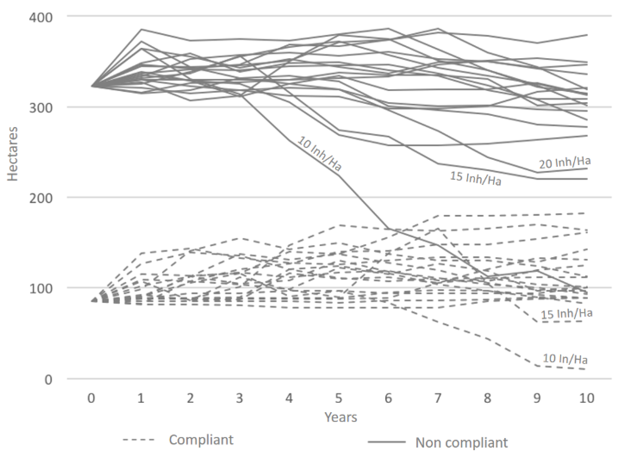
A summary of the experiments’ main findings is shown in Table 2, which is explained in detail below.

3.1. Total Attractive Land Footprint

It has always been considered by investors that the land available for industrial activity in the city of Ensenada is very limited, so an interest in this research was to know what could be the availability of Attractive Land compatible with the UDPE. More important was to identify where could Attractive Land rise with incompatibility with the UDPE but attractive for this activity, and thus try to foresee possible normative violations.

In this aspect, it is observed that there will always be more Attractive Land in normative incompatibility than in normative compatibility (Figure 4), but with a downward trend of the first and upward of the second until a time is reached when both types of Attractive Land descend uniformly. This shows that, as the city grows, the demand for industrial land use is higher than the available zoning for this activity established by the city’s UDPE. Something to note is that in the presence of low population densities between 10 to 20 inhabitants per hectare (Figure 5), Attractive Land drops steeply in a period of between 4 to 7 years, probably due to the fact that in low densities the surface of urban land is higher and therefore the probability for the urbanization and disappearance of Attractive Land is greater.

When studying the spatial overlap of all model executions, it is observed the emergence of an Attractive Land corridor along a regional road that communicates the northeast part of the city (Figure 6). This corridor presents a gradient that shows the direct relationship between the city’s proximity and the probability of its formation. Together with the urbanization heat map that shows northeast growth, reflects the Ensenada’s real-life situation where its growth in the last decade has been concentrated in that area. The limits of this corridor are only because the current model design works only within official city limits, which means that there is a high probability that it would extend beyond these limits in real life. According to the Attractive Land State heat map, there is a possibility of its urbanization by other land uses and not only by industry.

The heat map about Attractive Land to industry being occupied by this same activity (Figure 7) shows that this possibility is low in almost all parts of the city, even though there is ample opportunity for land occupation, mostly in incompatibility with the UDPE. There is a relevant exception to this condition in two zones, but to be able to develop them, the construction of regional roads is mandatory. It is observed that the development of these two zones located in the north and south ends of the city is not allowed by the UDPE despite that their location is desirable and contrary to the current situation where there are industrial uses in inner parts of the city.

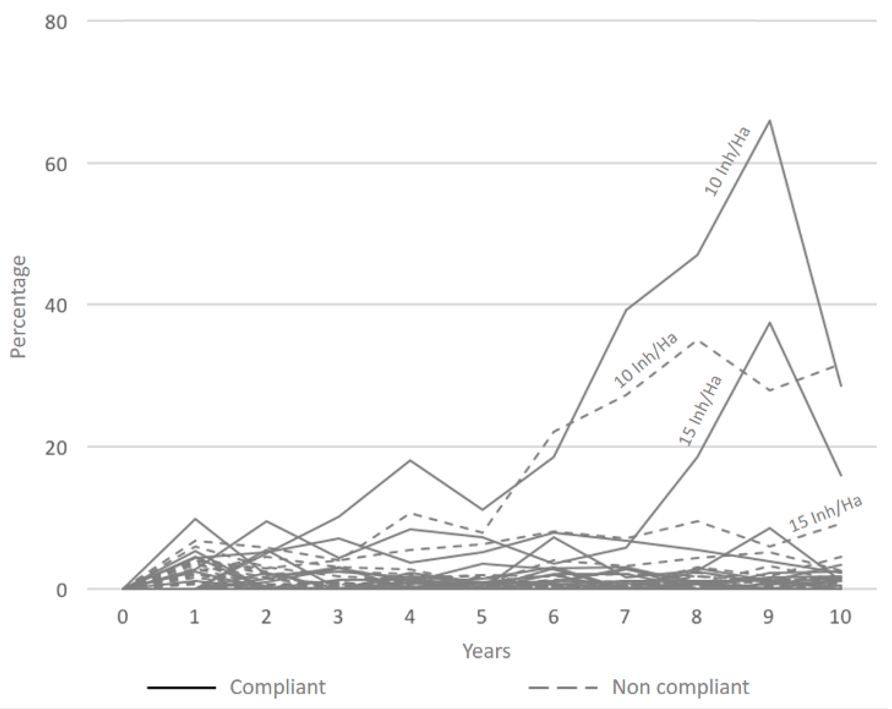
3.2. Percentage of Urbanized Attractive Land Footprints

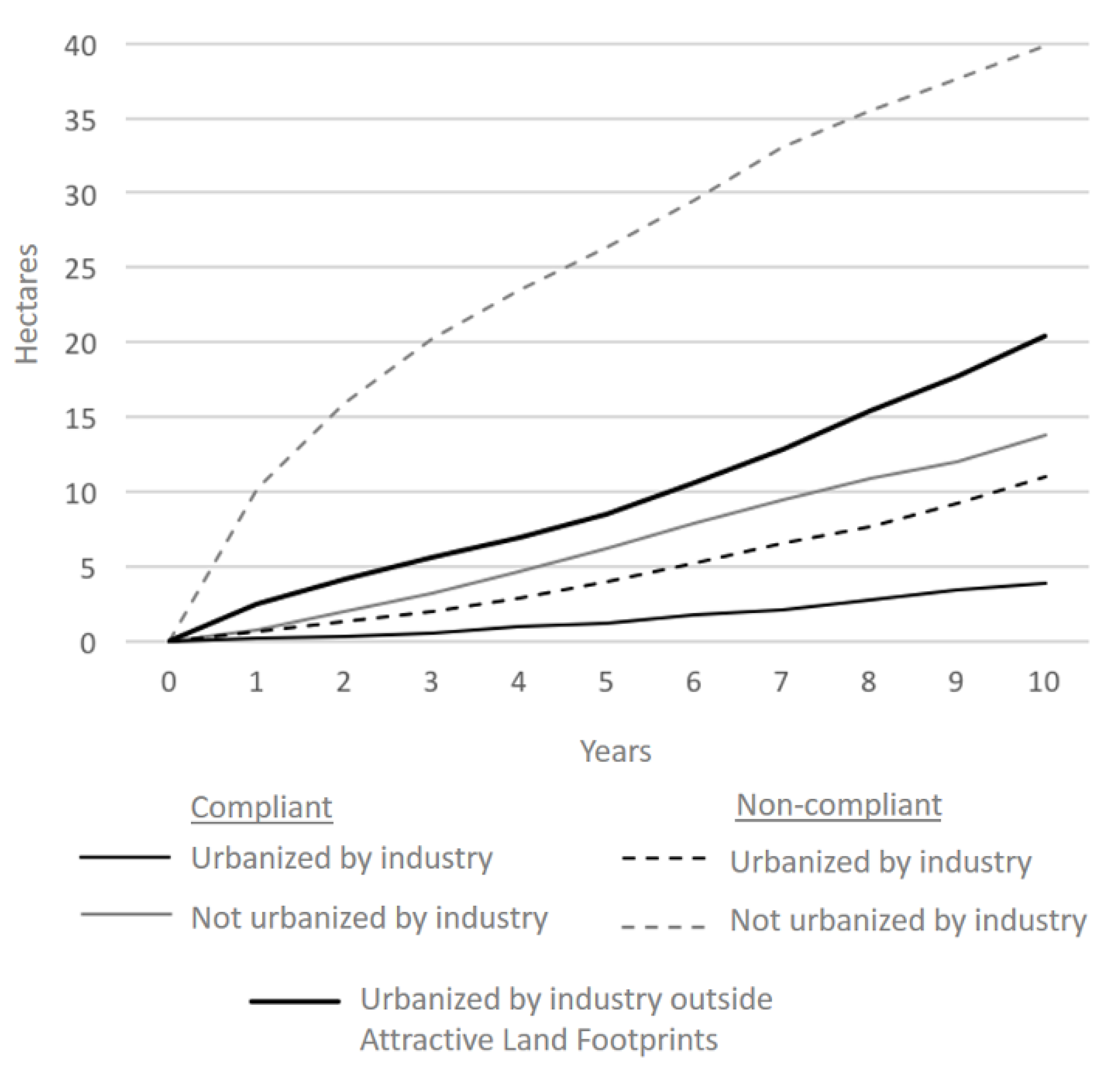
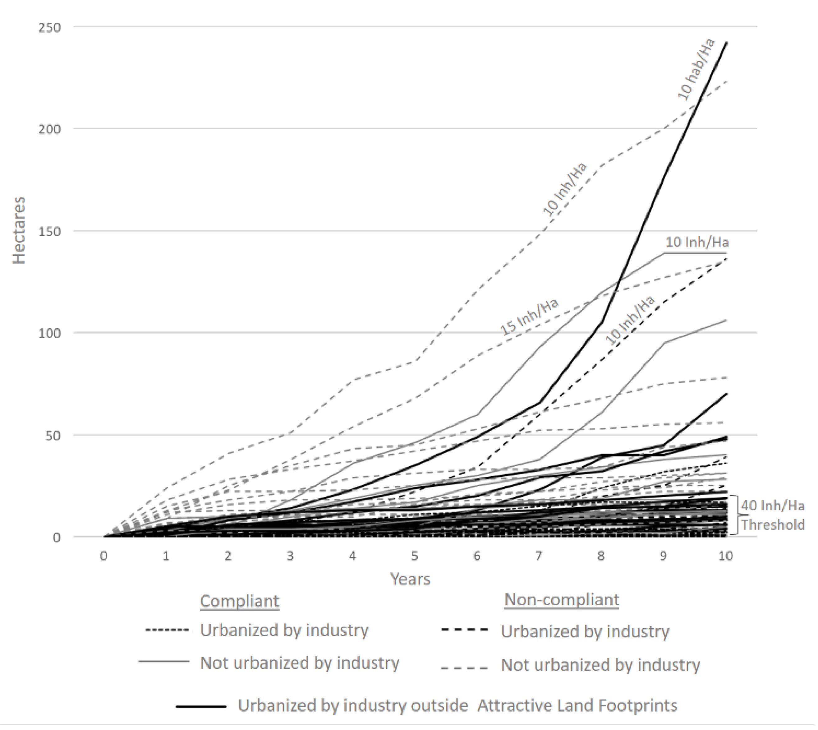
It outputs the percentage of Attractive Land that is urbanized in a given year. It was included in the model to know the dynamics of emergence-disappearance of Attractive Land and is complementary to the Urbanized Attractive Land output.

The behavior in each model run was so variable that it merited the individual analysis of each result, but relevant observations can be made in the context of density scenarios. In the presence of low densities of 10 to 15 inhabitants per hectare, urbanization of Attractive Land Footprints in a given year tends to increase by up to 65%, compared to up to 14% when 35 inhabitants per hectare, similar to Ensenada’s current density, was applied (Figure 8).

3.3. Urbanized Attractive Land Footprint Differentiated by Compatibility

This output quantifies the amount of Attractive Land that has been urbanized and that complies with urban regulations, but also identifies the one that does not comply and thus violates urban regulations. The intention of this indicator is to have support in the characterization of industry in normative incompatibility due to lack of appropriate industrial zoning or the lack of compliance with urban regulations, and in this way assess the need to add new zoning or complement industrial regulations.

Throughout the different executions of the model, it was observed that urbanization of Attractive Land Footprints by other land uses different to the industry predominates (Figure 9), which reduces the opportunities for it´s favorable location. Although a land cost variable is not included in the model, it nevertheless relates to a real-life situation in which most of the current industrial activities sit in more unfavorable locations due to high land costs. Contrary to a desirable situation, and according to the model, the lowest occupation scenario was that of industrial occupation in Attractive Land with normative compatibility.

In a low population density scenario between 10 to 20 inhabitants/ha, it was observed that the urbanization of Attractive Land Footprint rises rapidly, and occupied by non-industrial land uses (Figure 10). The rise of industrial occupation outside of Attractive Land was also noted. It is observed that in densities of approximately 40 Inhabitants/ha or higher, the total industrial surface outside of Attractive Land Footprint is low, which is a desired condition.

This finding is significant since the current density of the city of Ensenada is 35 inhabitants/ha, which means that is at a threshold that, if even lower densities surpass it, the industry will begin to appear more frequently in undesired places. This assumption is supported by the Sectorial Industrial Development Program of Ensenada [1] and the Partial Program of Urban Improvement of Downtown Seafront of Ensenada [49]. These programs established that the downtown area has both a low density of 11 inhabitants/ha and a high industrial use presence, even surpassing existing industry in peripheral areas that should be highly attractive in real life due to connectivity factors.

Spatially, there is a moderate possibility of Attractive Land urbanization in most of the city’s northeastern sector and those northern and southern areas previously identified as having a high probability of forming Attractive Land currently banned by the UDPE.

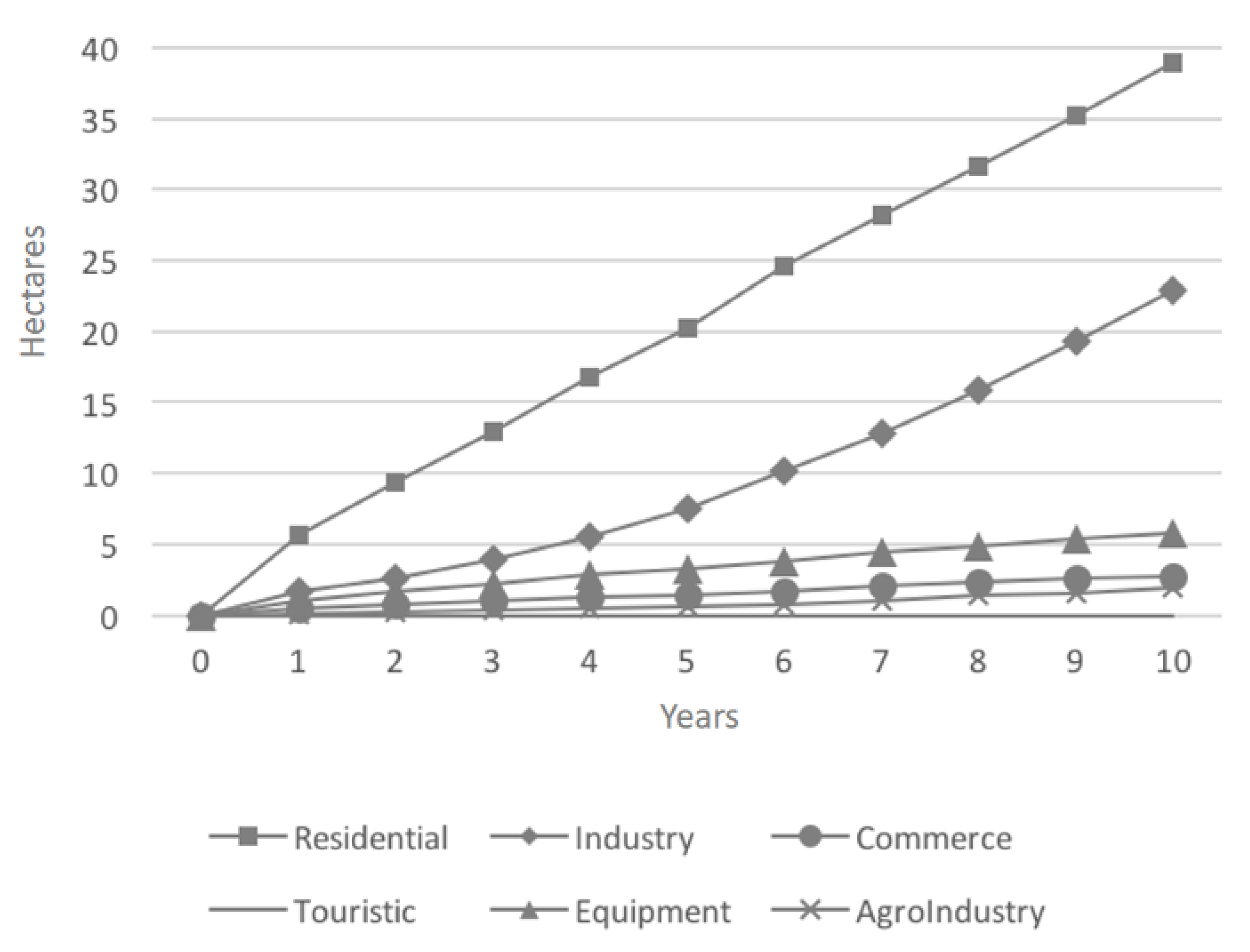
3.4. Urbanized Attractive Land Footprint Differentiated by Land Use

This output quantifies Attractive Land Footprint that has been urbanized, differentiated by the type of land use. It is intended to understand if there is a vacant land competition between industry and other land uses. Results outputted Ensenada’s current urban phenomenon of diminishing of proper vacant land for the industry due to residential occupation. Traditionally it has been considered that the location of residential use has been an inhibitor in industrial growth as they occupy zones initially intended for industry. The model outputs consistently, and with minimal variation between results, residential land use mostly occupies Attractive Land for industry (Figure 11). The model replicates an evident competition for vacant land between these two uses that occur in real life, even recently reflected in relevant social activism.

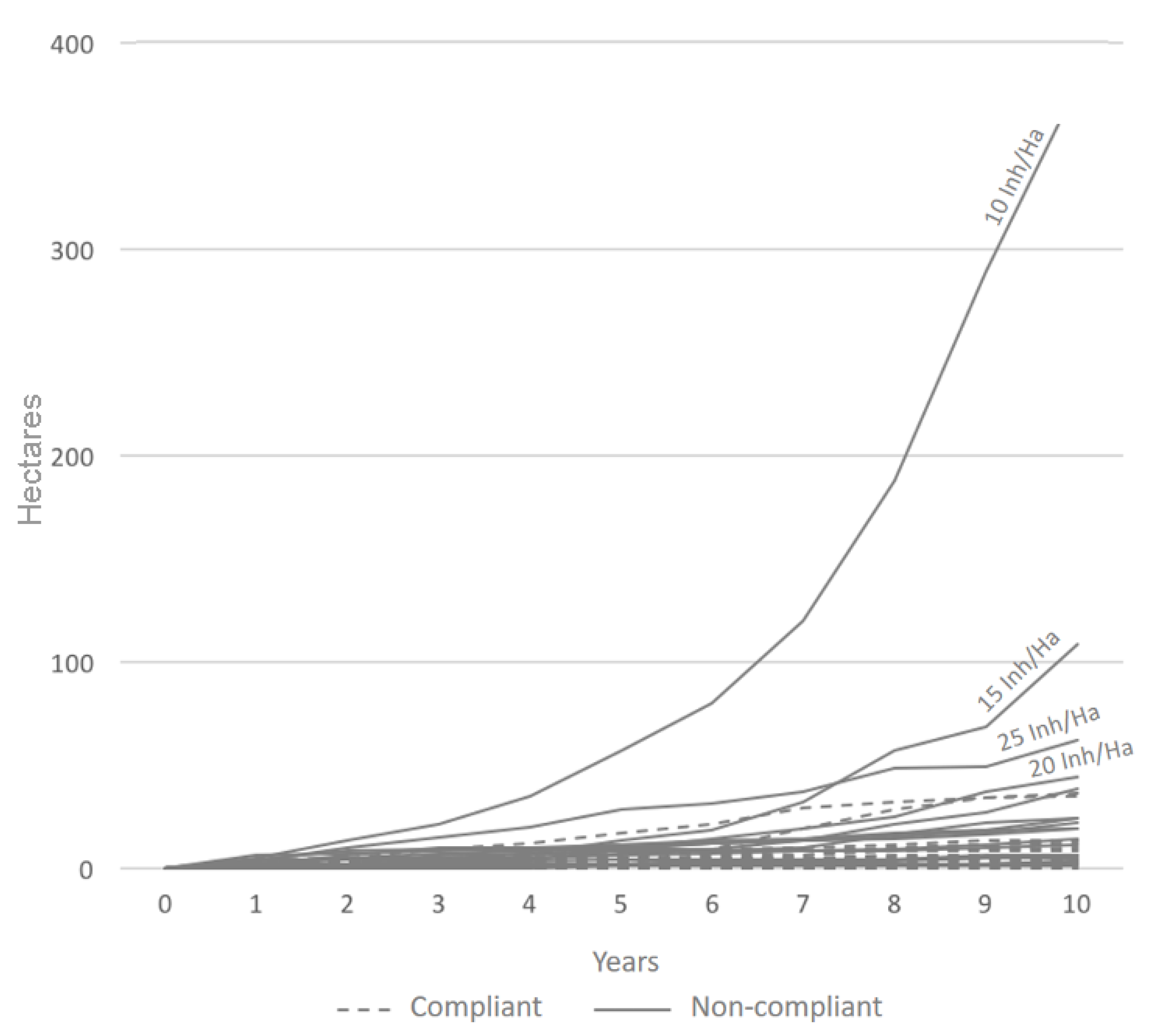
3.5. Industry Location Differentiated by Compatibility with the UDPE

This output quantifies built industrial surface that is compatible or incompatible with the UDPE and intends to know the amount of industry that is located in sub-sectors that are not compatible with this activity. If most industrial activity is located on incompatible sub-sectors, it denotes either an insufficient industrial zoning or regulation breaches. The model showed that in low densities between 10 to 25 hab/ha, the industrial surface in incompatible sub-sectors rises steeply in time (Figure 12).

In spatial terms, there is a particular interest that the model outputted zones with a high possibility of creating Attractive Land but conditioned to the noncompliance of the UDPE and the construction of a still projected road network.

3.6. Attractive Land Footprint States

This output quantifies the surface of Attractive Land that is “alive” or “dead”. Attractive Land is considered “alive” when it is vacant and fulfills desirability conditions for the industry. However, it is considered “dead” if it was urbanized or started having one or more neighboring land uses that are not desirable to be adjacent to industrial activities and thus stopped being alive. The interest in this indicator is to identify zones where there is a high urbanization of Attractive Land that can mean a high competition for land and consequently a need to regulate with more precision.

Results show that there is always a higher amount of Attractive Land Footprint that is alive in the initial years but then invariably goes down as dead surface rises until they are inverted and there’s is more dead than an alive surface (Figure 13).

According to the model, the year in which they are inverted is density-dependent, and it comes closer to the present as population densities are lowered. The rate at which alive surface diminishes is also density-dependent. When density is low, it immediately goes down at the same rate that the dead surface rises, but when density is high, the rates are significantly different as dead surface rises at a faster rate than the surface that is alive.

4. Conclusions

Through the use of the model presented in this paper, relevant topics to the efficient use of land were identified. Although some are industry-related only, others have a more generalized impact. As already discussed, these a relevant to population densities alternatives, having an important role in the gradual decrease of industry-attractive vacant land as low population densities produces sprawl that rapidly engulfs these Footprints. The effects of low densities on a particular land use had never been identified, so this finding complements the understanding of its impacts. The model also demonstrates how industry-attractive vacant land strongly depends on an efficient road infrastructure.

Another significant finding was how relevant UDPE regulations limits observed industry growth trends. It was observed that the UDPE would have to be breached if growth was to be stimulated in areas where a high possibility for industry-attractive vacant land was detected. This is further complicated because the model showed that there will always be more attractive land in sub-sectors where industrial activity is currently not allowed. This forces to revise the UDPE under this perspective: or more detailed and strict regulations are elaborated that inhibits this dissemination, or some of these areas must be recognized as new zoning for industrial growth. The model outputted areas with a high possibility of generating industry-attractive vacant land near yet to build residential developments, anticipating a competition for land occupation between these land uses, as it’s already happening in other parts of Ensenada city. This model then becomes a relevant justifier for redirecting the city’s current efforts in attracting a generic industry. Instead, a focus should be made on drawing specific industries that have a higher possibility of carrying out their activities near residential areas.

The results obtained by the simulations are encouraging regarding their usefulness, although adjustments will need to be made to adapt them to future exercises. Combining the results allows us to anticipate aspects of availability, occupation, location, competition, and vacant land legality attractive to the industrial real estate market.

Since the results are of interest to this sector and the government, these models can be a common point of communication, given their transparency and ease of modifying their structure and variables. Although both have a concern in industry-attractive vacant land, the interests are different: the first is to find the best options at the lowest cost and maximum benefit. The second is to find options that help design better territorial public policies and improve urban planning practice. But propositional feedback from industrial real estate developers shows that these differences will not be an obstacle for reaching conciliatory measures.

Although applying this model to other cities is feasible, specific considerations have to be resolved, which may be challenging to resolve in Latin American localities. The main one is the availability of updated, digitized, and revised information necessary to feed the model. Another is the calibration of the parameters of distances and adjacent uses that can behave differently according to each locality’s characteristics. Another limiting element is outdated urban development plans that are surpassed by a locality current needs. Finally, another limitation is the inherent lack of technical capacity of the personnel in charge of designing and updating urban regulations, which are also replaced every three years according to municipal governments’ changes, making it challenging to continue applying these urban models, let alone understand them.

In the model’s future work is to integrate real estate developers feedback. Their contributions have inadvertently reinforced the need for the complex systems approach by arguing how land acquisition variables continuously change in reaction to local and exogenous variables. Another adjustment is to integrate the land value variable since it is inseparable from the nature of the real estate purchase. If this variable is not accessible, it can be replaced with the property’s cadastral value, giving a spatial overview of the relative cost since it would indicate which land is more expensive than another, but it would not suggest by what amount. Another pending task is to refine the criteria of linear and radial distances, slopes, and the amounts of specific and desirable land uses to be considered by the model as attractive to an industrial real estate market. A user manual and interface design as user-friendly as possible will also be necessary to facilitate its use by the public official on duty. Finally, as is usually the case when creating a model, unexpected results were obtained in verification tests, as was the Land Use Compatibility Matrix case. When experimenting with simplified versions, it inhibited or stimulated specific land uses beyond what was proposed by the UDPE. This unexpected behavior demands further Matrix experimentation as its 6771 compatibility decisions have never been thoroughly tested. Nevertheless, it is still the primary decision tool for municipal authorities when granting land use permits, so the possible effects on the city could be contrary to those intended by the same UDPE. Because of the importance of this matter, it is now considered an urgent and new research opportunity.

Supplementary Materials

The Supplementary Materials are available online at https://www.mdpi.com/2071-1050/13/2/714/s1.

Author Contributions

Conceptualization and writing–original draft preparation J.S.-F. and M.C.-P.; investigation, resources, data curation, software, visualization, validation and formal analysis, J.S.-F.; methodology, supervision, M.C.-P.; writing–review and editing J.S.-F., M.C.-P. and C.G.G.-P.; project administration and funding acquisition, C.G.G.-P. All authors have read and agreed to the published version of the manuscript.

Funding

This research has been supported by the Universidad Autónoma de Baja California.

Institutional Review Board Statement

Not applicable.

Informed Consent Statement

Not applicable.

Data Availability Statement

Not applicable.

Acknowledgments

We would like to thanks “Universidad Autómoma de Baja California” and “Instituto Metropolitano de Investigación y Planeación de Ensenada” in México for supporting this project.

Conflicts of Interest

The authors declare no conflict of interest.

Abbreviations

The following abbreviations are used in this manuscript:

IMIP	Instituto Metropolitano de Investigación y Planeación del Municipio Ensenada
UDPE	Urban Development Plan of Ensenada
ALF	Attractive Land Footprints
ODD	Overview, Design Concepts, and Details protocol
ABM	Agent-Based Models
MAS	Multi-Agent Systems

Appendix A. Complementary Tables and Figures

Appendix A.1. Attractive Factors by Land-Use Type

Table A1. Attractive factors by land-use type.

Factor	Housing	Commercial	Industry	Tourism	Equipment
Job offer	•
Labour		•	•	•
Services	•	•	•	•
Cost of affordable land	•	•	•	•	•
Physical risk
Beach	•			•
Roads	•	•	•	•	•
Transfer time	•	•	•
Downtown centers	•	•
Transport systems	•	•	•		•
Existing development	•	•	•		•
Housing	•	•			•
Infrastructure	•	•	•	•	•
Building land	•	•	•	•	•
Income level		•
Elevation	•
Flood zones
Water bodies (Streams, lakes)	•			•
Industrial density		•	•
light industry		•
Urban sub-centers	•	•			•
Railway		•	•
Total saleable area		•	•	•
Green areas	•			•
Weather	•			•
Scenic views	•			•
Agricultural areas
Dumpsters
Urban periphery			•
Schools	•	•			•
Hospitals	•	•			•
Sports equipment	•	•			•
Soft slope	•		•
Zoning	•	•	•	•	•
Rural areas	•			•
Price of water			•	•
Housing density	•	•			•
Commercial density	•	•			•
Industrial density		•	•
Airports		•	•
Natural protected areas				•
Protected historical sites				•
Rights of way
Military facilities
Pantheons
Loading terminals		•	•

Appendix B. Modeling and Simulation Process

The methodology’s sequence is based on the well-known process in which a real-life target is selected and represented in a simplified way through a model that is executed and outputs data [17]. In more detail, it follows a process similar to the one presented by [48], which starts system analysis, conceptual modeling of the system, design of the simulation, generation of the code for the simulation, preparation of the simulation, execution of the simulation and ends with the analysis of the results (Figure A1).

Figure A1. Modeling and simulation process according to [48].

Appendix B.1. Data Requirements

For this methodology’s application, two main components are needed:

(1): Spatial data layers. They should be in SHP or ASC format, depending on the case (Table A2).
(2): Urban development plan applicable to the human settlement to be modeled. The spatial data layers and the Urban Development Plan (Table A3) must belong to the same time cut. Usually, the layers are derived from the work done to make the Plan.

Table A2. Spatial data layers needed for the model.

Data	Format	Type
City limits polygon	SHP	Vector
Citiy sub-sectors	SHP	Vector
Urban grid	SHP	Polygon
Water bodies	SHP	Polygon
Slope	SHP	Raster
Agricultural zones	SHP	Polygon
Developed land	SHP	Polygon
Developable land	SHP	Polygon
Non-developable land	SHP	Polygon
Road structure	SHP	Vector
Land use	SHP	Polygon

Table A3. Needed information from the Urban Development Plan.

Information	Type
Land Use Compatibility Matrix	Table
City limits polygon	Map
Sectors/subsectors	Map
Population historic growth	Table/Plot
Population growth projection	Table/Plot
Current urban surface	Table
Current land use surfaces	Table/Plot
Population growth rate	Table/Plot
% of industry compatible with Urban Development Plan regulation	Table/Plot
Population density (inhabitants per hectare)	Table

Appendix B.2. Data Preparation

The input data needed for the simulations must be prepared in a particular way to fit the current scope and limitations of the model, increasing flexibility for data input will be considered in future system modifications.

Appendix B.3. Land Use Compatibility Matrix

(1): Conditioned land uses. According to this model’s scope, to correctly read the Land-Use Compatibility Matrix, it must only contain compatibilities and incompatibilities concerning urban sub-sectors. The model does not accept conditioned uses, which are common in these matrices in Urban Development Plans. For this reason, it is necessary to evaluate which conditioned land uses will be converted into compatible or incompatible uses.
(2): Land uses that do not represent surfaces. Uses that do not manifest themselves as a surface in real life will be eliminated to avoid an erroneous spatial representation in the model results. Examples are bicycle paths added to existing roads which do not represent an additional urban area, ATMs that are an integral part of other land uses, or campsites that are temporary, seasonal, minimal, and removable.
(3): Unique or existing land uses. Care should be taken that the model does not result in land uses that are unique or have already been constructed after elaborating the Urban Development Plan. This information is entered, so no more instances are replicated once a land-use of this nature is built in a simulation. Examples of this type of land use are City Hall that only exists one per population center, Dam, Railroad, Market, and Regional Hospital. Population center size must be considered to determine whether a land use will be unique, under the logic that as the population is larger, the less likely it is to be unique.
(4): Urban corridors, urban centers and sub-centers. The model can read geographic spaces delimited by closed polygons and vectors, and therefore can read spatial information expressed in that way. Any other spatial expression expressed only in an indicative way and not represented by polygons or vectors will be eliminated from the compatibility matrix. Examples of these elements are the urban corridors that are usually marked as a point on the maps.

Appendix B.4. Spatial Data Layers

(1)

City’s polygon. Correspond with the polygon indicated in the Urban Development Plan.

(2)

City’s sub-sectors. Correspond with the sub-sectors of the Land Use Compatibility Matrix of the Urban Development Plan. The attributes table corresponding to this information layer must contain the following columns:

(a): SUB-SECTOR (which contains the sub-sector’s name of the corresponding polygon).
(b): COUNT (which contains the value 1 for all the sub-sectors, to differentiate in the model the territory inside the city’s polygon from the one outside)

(3)

Urban grid. It contains all the blocks and other urbanized areas included within the city’s polygon. The attributes table corresponding to this information layer must have the following column:

(a): URBAN (which contains the value 1 for each of the blocks and other urbanized areas of the city).

(4)

Water bodies. Correspond to lakes, dams, rivers, streams, and coasts within or adjacent to the city’s limits.

(5)

Slope. It is classified by range. If the Urban Development Plan has a threshold of urbanization concerning slopes, it must be manifested as a range limit.

(6)

Agricultural zones. They are the parcels that compose farms and cultivation areas. If there are other uses within them, they must be included. The attributes table corresponding to this layer of information must contain the following column:

(a): ZONING (which will contain the value 1 for each plot).

(7)

Developed land, non-developable land and developable Land. These three layers derive from the territorial aptitude model for the Urban Development Plan. If the model is unavailable, developed land data is obtained from the existing urban grid. Developable land is where no urbanization should be allowed for reasons of risk, conservation, or growth policies such as steep slopes, rivers, streams, coastal dunes, wetlands, geological faults, and outstanding natural areas. Developable land is the territory that remains on which it is possible to build according to urban policies that allow it.

(8)

Road structure. It is composed of roads and highways, differentiated in the corresponding layer’s attributes table. In-project roads are also included. The inclusion of secondary roads must be assessed if they could be used by heavy traffic. Local or service roads are excluded.

(9)

Land uses. It must contain the current land uses of the urban area. There must be a correspondence between these land uses and the Land Use Compatibility Matrix. The attribute table for this data layer must contain the following column:

(a): LAND_USE (which contains the name of the land use type of each polygon to which the value is assigned).

Appendix C. The Model

Appendix C.1. Overview, Design Concepts, and Details (ODD Protocol)

When simulation tools are required, the complexity approach uses multi-agent systems to formalize and test hypotheses about different aspects of their dynamics [26]. The methodology in this paper relies on Agent-Based Modeling (ABM) which focuses on individuals and on explaining how results can be achieved through their interactions, which makes it a good method for policy analysis [16].

The Attractive Land Footprints Agent-Based Model was developed in NetLogo, a widely used multi-agent programmable modeling environment [50]. The Figure A2 shows the NetLogo model interface.

Figure A2. Netlogo Model Interface: (1) Data loading and execution, (2) Initial condition parameters, (3) Attractive Land Footprint states, (4) Data layers display, (5) View, (6) Output plots, (7) Output export.

ABM is generally difficult to analyze, understand and communicate than other analytical models, so we will describe the model approaching the “Overview, Design Concepts, and Details” (ODD) protocol [51,52]. The ODD protocol for describing Agent-Based Models (ABMs) are now broadly accepted and used to document individual and multi-agent systems (MAS) models [47].

Overview

Purpose

The purpose of the model is to identify the emergence of specific spatial conditions as a result of aggregation behavior in an urban policy context. It demonstrates how the interaction of allowed urbanization regulations can result in an attractive environment for prohibited urbanization. The case in point is vacant land patterns that can attract industry (Attractive Land Footprints) by meeting requirements established from a developer’s perspective regardless of compliance to the Urban Development Plan of Ensenada (UDPE). These requirements include closeness to regional roads, workforce, urban equipment and not adjacent to residential areas. Due to the fact that the UDPE is currently under revision, this model is designed to be a tool to support the analysis and design of urban development policies by timely identifying zones where urban regulations may be infringed or even to discover unexpected opportunities, and adjust public policies accordingly.

Entities, State Variable and Scales

This is a grid based model representing the spatial extent of the city of Ensenada, México. Each cell of the model represents 10,000 m² or 1 hectare. The surface of the city’s polygon in which the model takes place is 45,652 hectares and is taken from the UDPE.

The entities of the model are of spatial nature and represent the city’s land use with variables that change over time. This takes place at the cell level, so 1 hectare is the basic spatial expression of this entity. The basic time unit is a year and the model is run in a 10-year span. These scales have been chosen because they are the ones used when designing and reviewing urban development plans.

(1): Low-level variables. These are variables that cannot be deduced from other low-level variables because they are elementary properties of the entity. Each cell of land contains the following low-level variables (Table A4).
(2): Attractive land. Attractive Land is not a land use but vacant land suitable for industry from a developer’s perspective. As such, in contrast to land uses that once they urbanize a cell is stays the same for the rest of the simulation, Attractive Land rises and diminishes on places that are urbanized or that aggregate favorable conditions for industry.
(3): Land use. It represents the activity that that takes place in the cell. It can be of 7 general types, or it can also be vacant, which means that there is no current activity. The 7 general types are subdivided into 111 specific land uses according to the UDPE. The 7 general types are Residential, Touristic, Industrial, Agro-Industrial, Commercial, Equipment, and Farmland. For visualization purposes, Industry land use appears as orange cells, and the rest of land uses are gray.
(4): Interest. It represents the interest of a cell to develop a land use. This interest can be one of the land uses specified in a UDPE´s Land Use Compatibility Matrix.
(5): Urban. Indicates if the cell is occupied by a land use.
(6): Row, column. Values that correspond to the location in the Land Use Compatibility Matrix and the Subsector being analyzed. These values are necessary so that the model can properly read this Matrix.
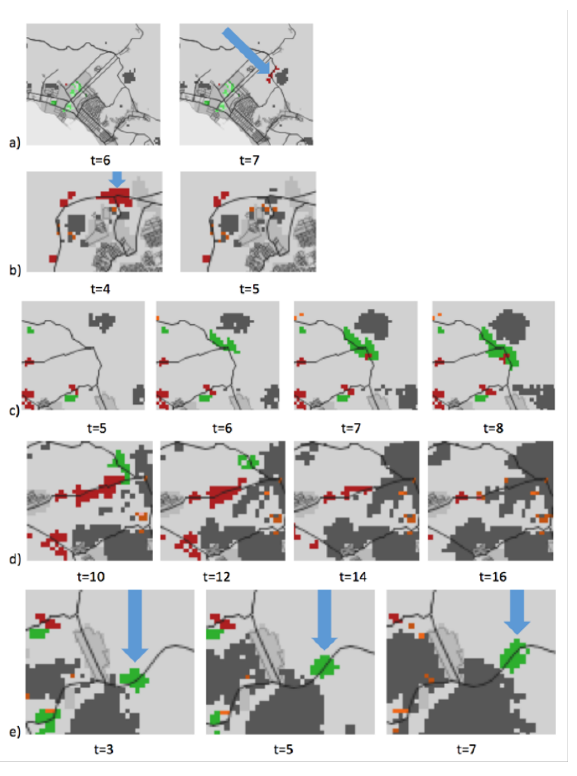
(7): Attraction. A value that specifies the level of attraction of a cell for industrial activities. The greater the value, the greater the attraction. The highest values are those that are considered as Attractive Land. Attractive Land is not a constructed land use but rather a vacant land that contains a specific set of characteristics that make it attractive for industrial use from a developer’s point of view. As such, and in contrast to urbanized land that remains in that state for the rest of the simulation, Attractive Land constantly changes its spatial pattern, or footprint, over time: it shrinks and disappears in areas that are gradually urbanized or emerges, grows and even moves where favorable conditions for the industry are agglomerated.
(8): Intersected by a street? It species whether the cell is intersected by a street/road or not. The Street/road network is obtained from the UDPE and includes current and projected network.
(9): Suitable? Conditions that must be met for a cell to be urbanized for any land use or can be considered Attractive Land. These conditions are: that the cell is inside city limits, that it is developable, that it is vacant, that it is not farmland, and that it is not a water body.
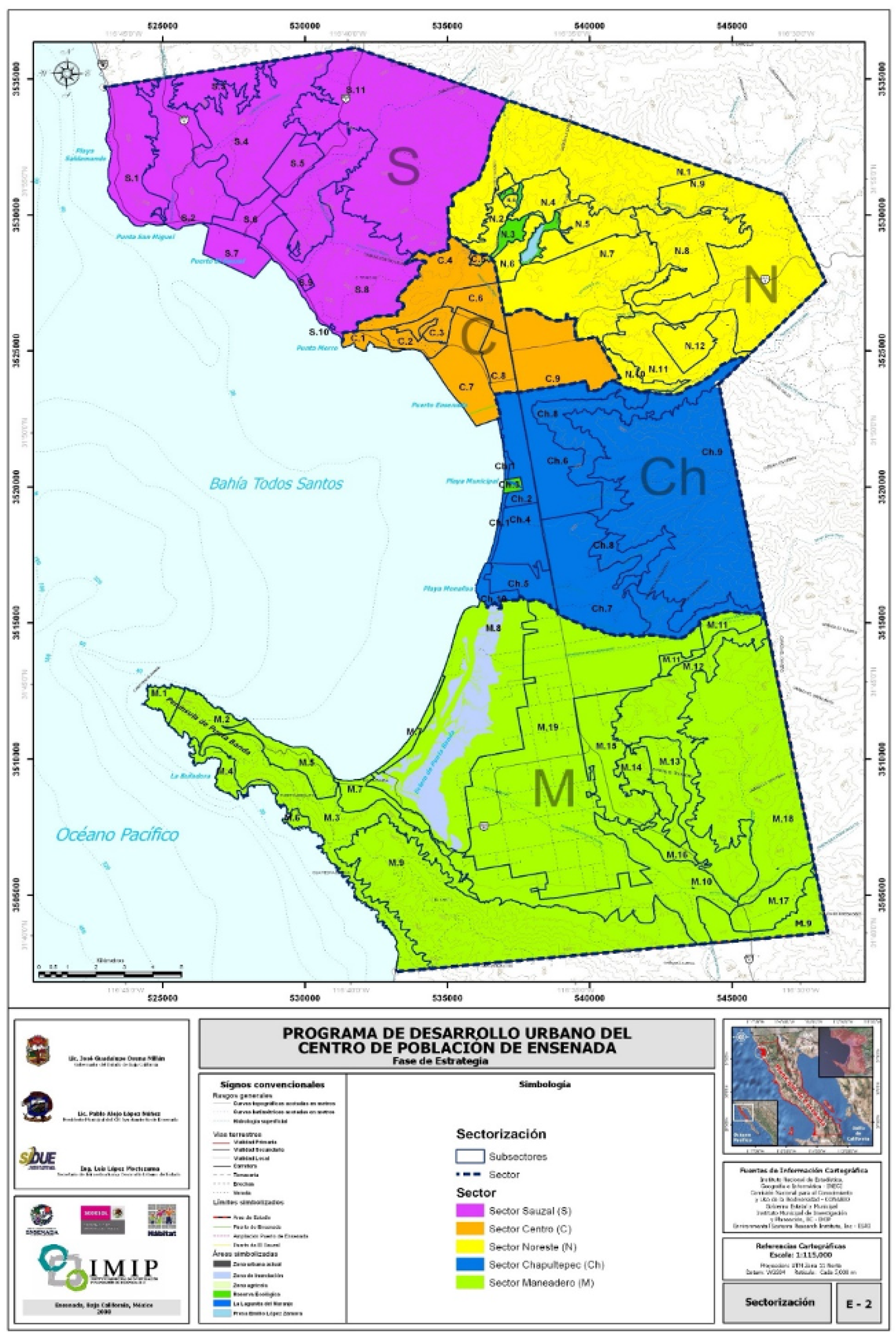
(10): City sub-sector. The city polygon is divided into 5 main sectors and subdivided in 61 sub-sectors according to the Urban Development Plan (Figure 2). The city limits polygon is greater than the current urban surface, so it also contains natural areas. Each one of the 111 specific land uses are compatible, or not, with each one of the 61 sub-sectors. Sub-sectors and compatibilities are taken from the Compatibility Matrix of the UDPE.
(11): Developable? The city’s polygon is composed of areas that are developable or non-developable. Non-developable areas represent streams, farmland, geologic faults, natural land, steep slopes and land 200 meters above sea level. The rest of the surface is developable land, including vacant lots inside the city. These areas are obtained from the UDPE.
(12): Potential random value that changes over time. It refers to the potential of vacant land to be developed. If this value is greater that an established threshold, the vacant land holding this value is urbanized and stays urbanized. Value is estimated according to the Vicsek-Szalay model that is later explained.
(13): Slope. It is the angle of terrain expressed in ranges: 1 = 0–5%, 2 = 0–10%, 3 = 0–15%, 4 = 0–30%, 5 > 30%.
(14): Body of water? It specifies if the cell is water.

There are also environmental variables that are not of spatial nature:

(1)

Potential threshold. All cells have a variable called Potential, which is continuously updated. An interest in developing a land use is assigned to cells that exceed this value previously established by the user.

(2)

Adjacency matrix. Matrix that specifies desired/undesired adjacency between land uses. It is designed from empirical evidence of land uses from the city of Ensenada.

(3)

Lawful industry percentage. From the total of times the model tries to grow industry in incompatible zones, this is the percentage of times the model will allow it. This does not necessary mean that industry will be built, because the terrain must satisfy a series of additional requirements for this land use.

(4)

Growth rate. Value that determines the average increase in the population. It is based on recent census data.

(5)

Years of development. The years the model will simulate.

(6)

Number of inhabitants. The model starts with a fixed population number according to recent census data, and is projected in a time span equal to Years of development variable. The amount of land uses that the model outputs depends on population size which in turn depends on the Population density variable.

(7)

Land use compatibility matrix. Matrix that specifies compatibility between each one of the 111 specific land uses and 61 subsectors, resulting in 6771 combinations. The concept of compatibility is not related to the adjacency of land uses, but to the permission of a land use to take place inside a city subsector, and is obtained from the Land Use Compatibility Matrix of the UDPE. In this sense, the compatibility of each cell with each one of the 111 land uses will depend on the subsector is in.

(8)

Population density. Inhabitants per hectare.

(9)

Slope restriction. Angle of terrain. Permitted slopes upon which urbanization can occur. Slopes are obtained from the UDPE.

(10)

Public policies. Actions to regulate urban growth. They are:

(a): Population density: Inhabitants per hectare.
(b): Slope restriction: Angle of terrain. Permitted slopes upon which urbanization can occur. Slopes are obtained from the UDPE.

Table A4. Entities and variables.

Type	Entity	Variables	Expression	Changes Over Time?
		Attractive land	Alive	Yes
		Attractive land	Dead	Yes
			Vacant	Yes
			Residential
			Touristic
			Industrial
		Land use	Agro-Industrial	No
			Commercial
			Equipment
			Farmland
			Residential
			Touristic
			Industrial
		Interest	Agro-Industrial	Yes
			Commercial
			Equipment
			Farmland
Grid cell	Land	Urban	Si	Yes
		Urban	No	Yes
		Row	Value established by the Compatibility Matrix	Yes
		Column	Value established by the Compatibility Matrix	Yes
		Attraction	Numeric value stated by model	Yes
		Intersected by a street?	Yes	No
		Intersected by a street?	No	No
		Suitable?	Yes	Yes
		Suitable?	No	Yes
		City sub-sector	Polygons established by the PDU	No
		Developable?	Yes	Yes
		Developable?	No	No
		Potential	Numerical value stated by sub-model	Yes
			0-5%
			0–10%
		Slope	0–15%	No
			0–30%
			>30%
		Body of water?	Yes	No
		Body of water?	No	No
	Urbanization threshold	Potential threshold	Numerical value stated by sub-model	Yes
	Land use neighbor preference	Adjacency Matrix	Desirable	No
	Land use neighbor preference	Adjacency Matrix	Not desirable	No
	Urban development program compliance	% Lawful industry	Numerical value stated by model user	No
		Growth rate	Numerical value stated by model user	No
Environment	Population	Years of growth	Numerical value stated by model user	No
		Number of inhabitants	Numerical value stated by model user	Yes
		Land use Compatibility Matrix	Compatible	No
		Land use Compatibility Matrix	Incompatible	No
		Population density	Numerical value stated by model user	No
	Public policies		0–5%	No
			0–10%
		Slope restriction	0–15%
			0–30%
			>30%

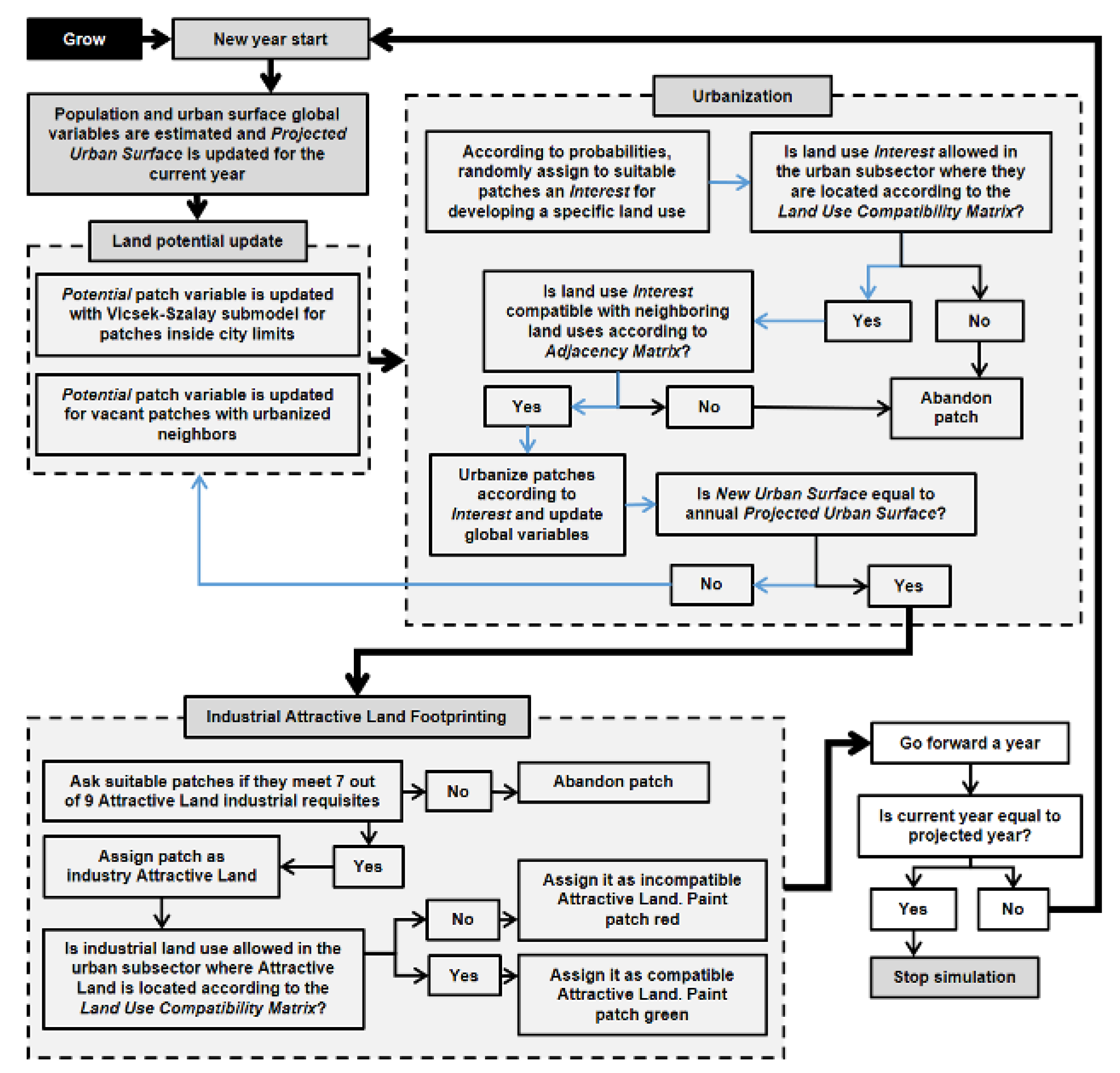
Process Overview and Scheduling

In this section the environmental and individual processes are presented as a concise overview of the model.

Figure A3. Model sequence.

(1): Setup. This is the first step of the model where pre-established numerical and spatial layers of data are loaded that together form the initial urban state of the model.
(2): Assign initial attractive land. Based on the initial spatial conditions of the model, it identifies the initial Attractive Land.
(3): Assign random value to cells. The model randomly assigns a value of 1 or -1 to a cell variable called Potential to all cells that are inside of the city polygon. This will be the base for the Vicsek-Szalay sub-model which determines if a vacant cell has potential for urbanization. Each land use has location requirements, mainly its compatibility to sub-sectors of the city and its preference to neighbor land uses (See Table A5).
(4): Estimate amount of projected urban surface. Based on initial population, growth rate, and population density, and amount of urban surface is projected for one year. The simulation stops once the current year equals the Years of development variable.
(5): Compare current vs projected urban surface. Projected urban surface is compared to growing urban surface. While the growing urban surface does not match projected urban surface, model will loop the following steps. If this condition is met, it exits the loop, advances by one year, plots and spatial pattern of land-uses is updated, and starts a new loop by estimating new projected urban surface.
(6): Update potential variable for each cell. All cells update their Potential variable according to the Vicsek-Szalay model. Additionally, urbanized cells rise the Potential variable of neighboring vacant cells. If the final value of this variable is higher than an stabilised threshold, only cells meeting this requirement proceed to the next step.
(7): Assign random land-use interest to cells with potential above threshold value. One of 111 possible land-uses is randomly assigned as a land use interest to the cells above threshold. It is assigned according to pre-established probabilities and represents an interest of the cell to develop that land-use. The probabilities are based on the proportion of land uses stated as current by the UDP.
(8): Validate the assigned land use with the compatibility matrix. The model verifies with the Land Use Compatibility Matrix if the randomly assigned land use interest is compatible with the sub-sector it’s in. If its compatible, proceeds to next step.
(9): Verify neighbors. The model verifies with the Adjacency Matrix that neighboring requirements by the land use interest can be met.
(10): Urbanize cell with land-use interest. If compatibility and requirements are fully satisfied, the cell is urbanized with the land-use interest, and Land Use, Developable?, Suitability, Farmland and Urban cell variables are updated. The last three are high-level variables that are deduced from low-level variables previously explained. Suitability establishes if a cell can be urbanized taking into account public policies, developable and vacant land and if its inside the city polygon. Farmland states if the cell is used for agricultural activities and Urban if the cell is occupied by a land-use. A global variable called New Urban Surface is also updated each time a cell is urbanized.
(11): Compare current urban surface with projected urban surface. If current urban surface has not reached the projected urban surface, the loop remains by starting a new Update potential variable for each cell step. If it does, exits the current year loop and proceeds to the next step.
(12): Update attractive land. Based on the current spatial configuration of land uses, the model updates location and amount of Attractive Land.
(13): Compare current year with years of development variable. If current year is the same as Years of development variable, the model stops and the spatial pattern of land-uses is updated, along with plots and monitors.

Table A5. Adjacency Matrix.

		Residential	Touristic	Industrial	Agro-Industrial	Commercial		Equipment		Beach
		Residential	Touristic	Industrial	Agro-Industrial	Commercial Industry Compatible	Commercial Industry Incompatible	Commercial Industry Compatible	Commercial Industry Incompatible	Beach
Residential		O	O	X	X	O	O	O	O	O
Touristic		O	O	X	X	O	O	O	O	(2)
Industrial		X	X	O	O	O	X	O	X	O
Agro-industrial		X	X	O	O	O	O	O	O	O
Commercial	Commercial Industry compatible	(1)	O	O	O	O	O	O	O	O
Commercial	Commercial Industry incompatible	(1)	O	X	X	X	O	X	O	O
Equipment	Commercial Industry compatible	(1)	O	O	O	O	O	O	O	O
Equipment	Commercial Industry incompatible	(1)	O	X	X	O	O	O	O	O

X no neighbors accepted. O neighbors accepted. (1) As long as there are two or more residential neighbors. (2) As long as there are one or more beach neighbors in a radius of 5 cells.

Appendix C.2. Design Concepts

Appendix C.2.1. Basic Principles

The basic principle of this model is that of cellular automata and how the state of a cell is determined by the state of its neighbors, and by environmental variables that represent public policies, population growth and compatibility rules established by an official Urban Development Plan.

Emergence

Vacant land is going to be attractive to one or several land-uses depending on its location with respect to spatial patterns of land-use that surrounds it and to environmental variables. The behavior in quantity and spatial distribution of Attractive Land will vary over time. A cell of land is attractive to more than one land-use at the same time, so the quantity and location of Attractive Land for industry will diminish as it is taken by other land-uses but also arise in other zones where favorable conditions aggregate.

Interaction

Interaction in the model is between land-uses and land-uses with its surroundings. This interaction is based on the neighborhood concept. Depending on its type, land-uses can or cannot be adjacent to each other, so once a land-use is stabilised it creates conditions around it that are favorable to some land-uses and unfavorable to others. Also, once a land-use urbanizes a vacant cell, it changes its Urban, Suitability and Farmland variables and raises the Potential variable of surrounding vacant cells.

Stochasticity

A land-use interest is randomly assigned to cells that its Potential variable is above a threshold value. The frequency on which a specific land use is randomly assigned depends on pre-established probabilities.

Collectives

Attractive Land spatially aggregate according to industry-specific requirements, forming particular patterns and land-use spatial distributions.

Observation

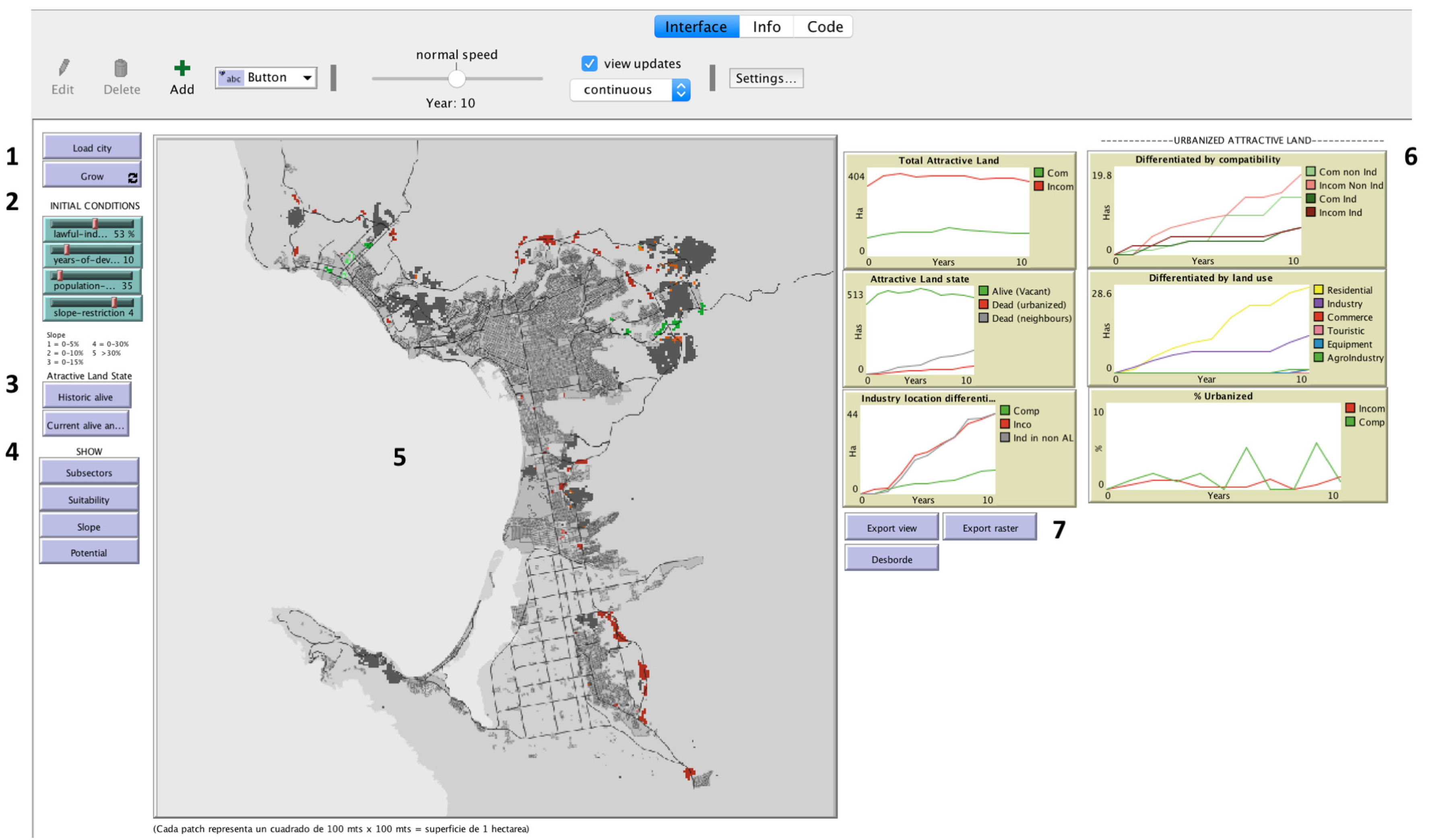
The model outputs an image of land-use patterns of industry, Attractive Land Footprints and general land uses. It also plots the following data:

(1): Total Attractive Land.
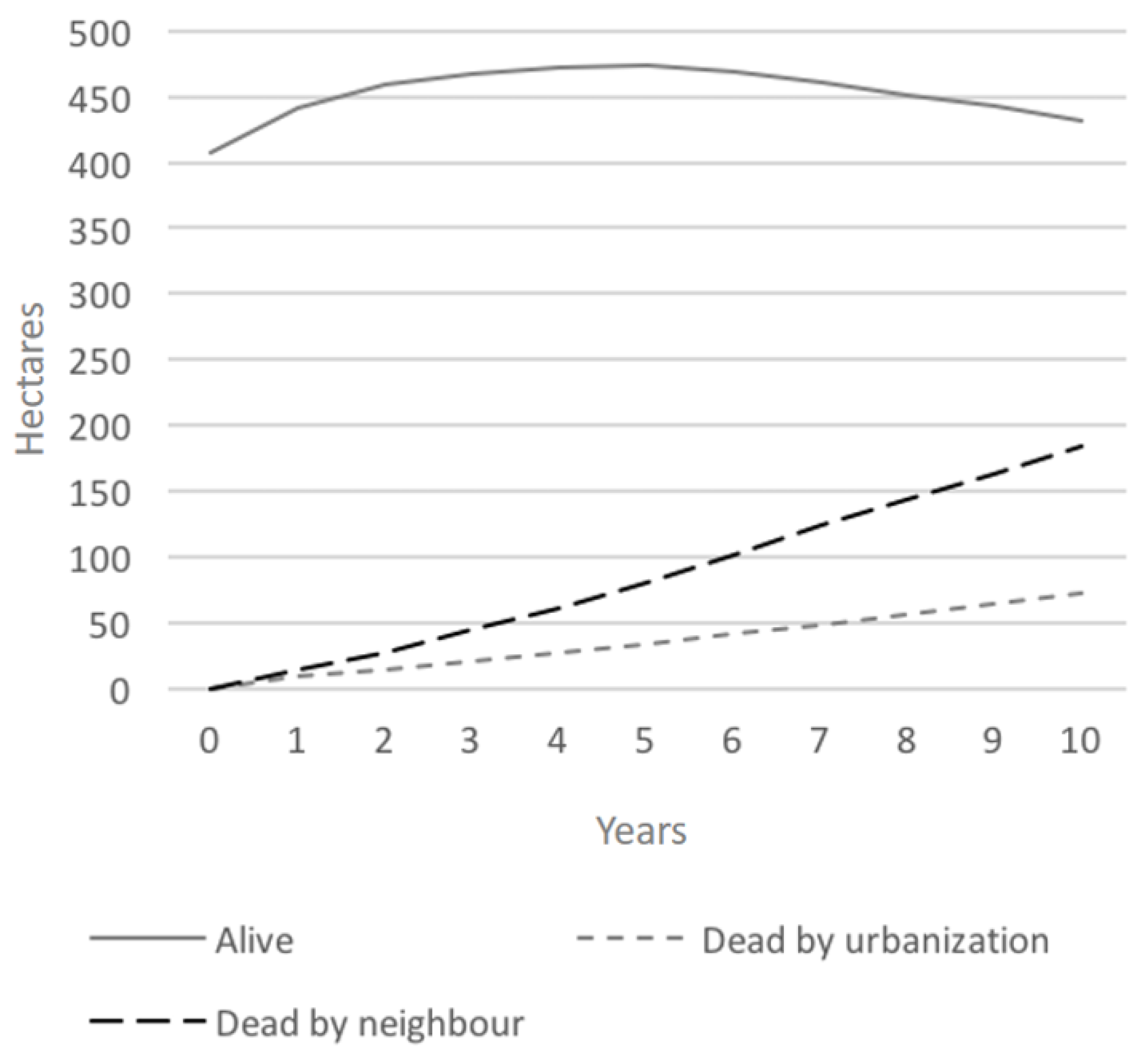
(2): Attractive Land State.
(3): Industry location differentiated by compatibility.
(4): Urbanized Attractive Land differentiated by: Compatibility, land use and percentage urbanized.

The steep topography that surrounds the city dramatically limits its growth and has had a historical influence on current urban shape. Regarding the model, topography has a relevant influence on the parameter space of the final urban shape, which is rather low. An overlay of urban patterns that resulted from 500 individual simulations were analyzed, and it was detected that by approximately the 50th overlay no noticeable differences were identified beyond this point, so for output analysis, an exercise of 50 runs was made.

Appendix C.2.2. Details

Attractive Land

A cell in the model is considered as Attractive Land when it fulfills at least 7 of the following 9 requisites:

(1): Land slope equal or lower than 15%.
(2): 0 neighbors of residential land use.
(3): 0 neighbors of touristic land use.
(4): 0 neighbors of commercial land use that does not want to be adjacent to industry.
(5): 0 neighbors of equipment land use that does not want to be adjacent to industry.
(6): A regional road within a 2-cell radius.
(7): 20 or more cells of residential land use within a 20-cell radius.
(8): 4 or more cells of industrial land use within a 2-cell radius.
(9): 2 or more cells of industrial land use in a 1 cell radius.

A cell is no longer Attractive Land for industry once one or more of the following happens:

(1): 1 or more neighbors of residential land use.
(2): 1 or more neighbors of touristic land use.
(3): 1 or more neighbors of commercial land use that does not want to be adjacent to industry.
(4): 1 or more neighbors of equipment land use that does not want to be adjacent to industry.

Moore neighborhood is used when inspecting for neighbors.

Initialization

The model initially detects Attractive Land according to previously stated requisites (Figure A4).

Figure A4. Initial state of the model, showing the spatial extent of the city of Ensenada and Attractive Land Footprints for industry in compatibility (green) and incompatibility (red) with the UDPE.

Input Data

Initial values for simulation where as follows:

(1): Initial population: 363,260. Taken from the most recent census data.
(2): Growth rate: 1.7. Obtained from the UDPE.
(3): Lawful industry percentage: 53%. It was obtained from the Sectorial Industrial Development Program of Ensenada, which states that 47% of industry is located against urban regulations of the UDPE.
(4): Years of development: 10. It is a time span in which it was considered by policy makers as adequate in a planning-revision context.
(5): Population density: 35. It’s the current Ensenada’s average density according to the UDPE.
(6): Slope restriction: 4. It corresponds to a slope range from 0 to 30%, which is close to current permitted urbanization on slopes not greater than 35% stated in the UDPE. The exact 35% value was not used due to technical challenges with available terrain data.
(7): Threshold: 4. The value for the Vicsek-Szalay sub-model was chosen after empirical observation of values that better approximated Ensenada’s morphology.

Current land-uses, developable and non-developable land, slope, and street and road networks, including those that are on a planning phase, are loaded in the model. This data layers are loaded as shp (vector) or asc (raster) layers previously elaborated in a Geographic Information System software for the UDPE.

Sub-Models

Vicsek-Szalay sub-model This sub-model updates all cells Potential variable. It is used to determine whether a vacant cell reaches the potential to be urbanized. For this to happen, the vacant cell potential must surpass an established threshold value. It is a cell based model that shows how highly ordered spatial patterns similar to those of urban development can emerge from a model that builds on spatial averaging [53]. This build patterns over time depending on a potential and threshold value. Potential can be translated to urbanization. This urbanization persists even if cell potential falls below the threshold value in the future. This pure averaging model is stated as

z_{i} (t + 1) = 1 / 5 [z_{i} (t) + \sum_{j \in N_{i}} z_{j} (t)] + ϵ_{i} (t)

It is a model that never moves to equilibrium because noise is constantly introduced into the system.

Besides the Vicsek-Szalay submodel, the Potential variable is also updated by neighboring urbanized cells as a way to replicate real-life situations where urban areas tend to urbanize adjacent vacant surfaces.

References

IMIP. Programa Sectorial de Desarrollo Industrial de Ensenada; Instituto Metropolitano de Investigación y Planeación del Municipio Ensenada; Enseanda: Baja California, México, 2017. [Google Scholar]
IMIP. Programa de desarrollo urbano de centro de población de Ensenada 2030. Periódico Oficial del Estado Baja California 2009, CXVI, 7–133. [Google Scholar]
Economía, S.D. Norma Mexicana NMX-R-046-SCFI-2015 Parques Industriales—Especificaciones Industrial Parks-Specifications. Diario Oficial de la Federación 2017, 07/03/2017, 1–44. [Google Scholar]
Bueno-Suárez, C.; Coq-Huelva, D. Sustaining what is unsustainable: A review of urban sprawl and urban socio-environmental policies in North America and Western Europe. Sustainability 2020, 12, 4445. [Google Scholar] [CrossRef]
Bosch, M.; Chenal, J.; Joost, S. Addressing Urban Sprawl from the Complexity Sciences. Urban Sci. 2019, 3, 60. [Google Scholar] [CrossRef] [Green Version]
Mitchell, M. Complexity: A Guided Tour, 1st ed.; Oxford University Press: New York, NY, USA, 2009; p. 349. [Google Scholar] [CrossRef] [Green Version]
Filatova, T. Empirical agent-based land market: Integrating adaptive economic behavior in urban land-use models. Comput. Environ. Urban Syst. 2015, 54, 397–413. [Google Scholar] [CrossRef]
Edmonds, B.; Meyer, R. Simulating Social Complexity: A Handbook, 1st ed.; Springer: Manchester, UK, 2013; p. 745. [Google Scholar]
Weiler, R.; Engelbrecht, J. The new sciences of networks & complexity: A short introduction. Cadmus J. 2013, 2, 131–141. [Google Scholar]
Beheshti, R.; Sukthankar, G. A Hybrid Modeling Approach for Parking and Traffic Prediction in Urban Simulations; Springer: Berlin/Heidelberg, Germany, 2014. [Google Scholar] [CrossRef]
Easley, D.; Kleinberg, J. Networks, crowds, and markets: Reasoning about a highly connected world. Science 2010, 81, 744. [Google Scholar] [CrossRef]
Morcol, G. Urban sprawl and public policy: A complexity theory perspective. Emerg. Complex. Organ. 2012, 14, 1–16. [Google Scholar]
Batty, M. Cities as Complex Systems: Scaling, Interaction, Networks, Dynamics and Urban Morphologies. In Encyclopedia of Complexity and Systems Science; Springer: London, UK, 2009; pp. 1041–1071. [Google Scholar] [CrossRef] [Green Version]
Portugali, J.; Meyer, H.; Stolk, E.; Tan, E. (Eds.) Complexity Theories of Cities Have Come of Age, 1st ed.; Springer: Berlin/Heidelberg, Germany, 2012; p. 438. [Google Scholar] [CrossRef] [Green Version]
Atun, F. Understanding effects of complexity in cities during disasters. In Understanding Complex Urban Systems: Multidisciplinary Approaches to Modeling; Walloth, C., Gurr, J.M., Schmidt, J.A., Eds.; Springer: Berlin/Heidelberg, Germany, 2014; Volume 106, pp. 51–65. [Google Scholar] [CrossRef]
Furtado, B.A.; Sakowski, P.A.M.; Tovolli, M.H. Modeling Complex Systems for Public Policy, 1st ed.; Institute for Applied Economic Research: Brasília, Brazil, 2015; Volume 37, p. 396. [Google Scholar]
Gilbert, N.; Troitzcsch, K.G. Simulation for the Social Scientist, 2nd ed.; Open University Press: Glasgow, Scotland, 2005; p. 295. [Google Scholar]
OECD; Global Science Forum. Applications of Complexity Science for Public Policy: New Tools for Finding Unanticipated Consequences and Unrealized Opportunities; Technical Report September; The Organisation for Economic Co-operation and Development: Erice, Sicily, 2009. [Google Scholar]
Goldstein, J. Emergence as a Construct: History and Issues. Emergence 1999, 1, 49–72. [Google Scholar] [CrossRef]
Portugali, J. Complexity, Cognition and the City, 1st ed.; Springer: Berlin/Heidelberg, Germany, 2011; p. 421. [Google Scholar]
Bazzanella, L.; Canerapo, L.; Corsiso, F.; Roccasalva, G. The future of cities and regions: Simulation, scenario and visioning, governance and scale. In Springer Geography; Bazzanella, L., Caneparo, L., Corsico, F., Roccasalva, G., Eds.; Springer: Berlin/Heidelberg, Germany, 2012. [Google Scholar]
Huang, J.; Zhang, J.; Lu, X.X. Applying SLEUTH for Simulating and Assessing Urban Growth Scenario Based on Time Series TM Images: Referencing To a Case Study of Chongqing, China. Int. Arch. Photogramm. Remote. Sens. Spat. Inf. Sci. 2008, 37, 597–606. [Google Scholar]
Hossain, S.; Scholz, W.; Baumgart, S. Translation of urban planning models: Planning principles, procedural elements and institutional settings. Habitat Int. 2015, 48, 140–148. [Google Scholar] [CrossRef]
Amato, F.; Pontrandolfi, P.; Murgante, B. Supporting planning activities with the assessment and the prediction of urban sprawl using spatio-temporal analysis. Ecol. Inf. 2015, 30, 365–378. [Google Scholar] [CrossRef]
Norte, N.; Pais, A. Cellular automata and urban studies: A literature survey. ACE Archit. City Environ. 2007, 1, 368–399. [Google Scholar] [CrossRef] [Green Version]
Bretagnolle, A.; Daudé, E.; Pumain, D. From Theory to Modelling: Urban Systems as Complex Systems. Cybergeo Rev. Eur. GéOgraphie / Eur. J. Geogr. 2006, 1–17. [Google Scholar] [CrossRef]
Inostroza, L.; Baur, R.; Elmar, C. Urban Sprawl and Fragmentation in Latin America: A Comparison with European Cities. The Myth of the Diffuse Latin American City; Working Paper LRB082510; Lincoln Institute of Land Policy: Cambridge, MA, USA, 2010. [Google Scholar]
Crooks, A.; Patel, A.; Wise, S. Multi-agent systems for urban planning. In Technologies for Urban and Spatial Planning: Virtual Cities and Territories; IGI Global: Pennsylvania, PA, USA, 2014; pp. 29–56. [Google Scholar] [CrossRef]
Watkiss, B.M. The SLEUTH Urban Growth Model as Forecasting and Decision-Making Tool. Ph.D. Thesis, Stellenbosch University, Stellenbosch, South Africa, 2008. [Google Scholar]
Barredo, J.I.; Kasanko, M.; McCormick, N.; Lavalle, C. Modelling dynamic spatial processes: Simulation of urban future scenarios through cellular automata. Landsc. Urban Plan. 2003, 64, 145–160. [Google Scholar] [CrossRef]
Healey, P. Urban Complexity and Spatial Strategies: Towards a Relational Planning for Our Times; Routledge: Abingdon, UK, 2008; p. 319. [Google Scholar] [CrossRef]
Abdullah, J. City Competitiveness and Urban Sprawl: Their Implications to Socio-Economic and Cultural Life in Malaysian Cities; Elsevier: Amsterdam, The Netherlands, 2012. [Google Scholar] [CrossRef] [Green Version]
Oryani, K.; Harris, B. Review of Land Use Models: Theory and Application. In Proceedings of the Sixth TRB Conference on the Application of Transportation Planning Methods, Oakland, AC, USA, 6 May 1997; pp. 80–91. [Google Scholar]
Walloth, C.; Gurr, J.M.; Schmidt, J.A. (Eds.) Understanding Complex Urban Systems: Multidisciplinary Approaches to Modeling, 1st ed.; Springer: Cham, Switzerland, 2014; p. 158. [Google Scholar]
Lechner, T.; Ren, P.; Watson, B.; Brozefski, C.; Wilensky, U. Procedural Modeling of Urban Land Use. In ACM SIGGRAPH 2006 Research Posters; Association for Computing Machinery: New York, NY, USA, 2006; p. 135-es. [Google Scholar] [CrossRef] [Green Version]
Santé, I.; García, A.M.; Miranda, D.; Crecente, R. Cellular automata models for the simulation of real-world urban processes: A review and analysis. Landsc. Urban Plan. 2010, 96, 108–122. [Google Scholar] [CrossRef]
Xia, L.; Gar-On, Y. Integration of Principal Components Analysis And Cellular Automata for Spatial Decision-Making and Urban Simulation. Sci. China Ser. D Earth Sci. 2002, 45, 521–529. [Google Scholar] [CrossRef]
Fotheringham, A.S.; Rogerson, P.A. (Eds.) The SAGE Handbook of Spatial Analysis; Sage: Newcastle upon Tyne, UK, 2009; p. 526. [Google Scholar]
Hosseinali, F.; Alesheikh, A.A.; Nourian, F. Agent-based modeling of urban land-use development, case study: Simulating future scenarios of Qazvin city. Cities 2013, 31, 105–113. [Google Scholar] [CrossRef]
Hjorth, A.; Wilensky, U. Redesigning Your City—A Constructionist Environment for Urban Planning Education. Proc. Constr. 2014, 13, 1–10. [Google Scholar] [CrossRef]
Ligmann-Zielinska, A.; Jankowski, P. Exploring normative scenarios of land use development decisions with an agent-based simulation laboratory. Comput. Environ. Urban Syst. 2010, 34, 409–423. [Google Scholar] [CrossRef]
Vliet, J.V.; White, R.; Dragicevic, S. Modeling urban growth using a variable grid cellular automaton. Comput. Environ. Urban Syst. 2009, 33, 35–43. [Google Scholar] [CrossRef]
Arsanjani, J.J.; Helbich, M.; Kainz, W.; Boloorani, A.D. Integration of logistic regression, Markov chain and cellular automata models to simulate urban expansion. Int. J. Appl. Earth Obs. Geoinf. 2011, 21, 265–275. [Google Scholar] [CrossRef]
Paveglio, T.B.; Prato, T.; Hardy, M. Simulating effects of land use policies on extent of the wildland urban interface and wildfire risk in Flathead County, Montana. J. Environ. Manag. 2013, 130, 20–31. [Google Scholar] [CrossRef] [PubMed]
Portugali, J. Complex Artificial Environments: Simulation, Cognition and VR in the Study and Planning of Cities; Springer: Berlin/Heidelberg, Germany, 2006; pp. 219–233. [Google Scholar] [CrossRef]
Loibl, W.; Toetzer, T. Modeling growth and densification processes in suburban regions - Simulation of landscape transition with spatial agents. Environ. Model. Softw. 2003, 18, 553–563. [Google Scholar] [CrossRef]
Grimm, V.; Railsback, S.F.; Vincenot, C.E.; Berger, U.; Gallagher, C.; DeAngelis, D.L.; Edmonds, B.; Ge, J.; Giske, J.; Groeneveld, J.; et al. The ODD Protocol for Describing Agent-Based and Other Simulation Models: A Second Update to Improve Clarity, Replication, and Structural Realism. J. Artif. Soc. Soc. Simul. 2020, 23, 7. [Google Scholar] [CrossRef] [Green Version]
Garro, A.; Russo, W. EasyABMS: A domain-expert oriented methodology for agent-based modeling and simulation. Simul. Model. Pract. Theory 2010, 18, 1453–1467. [Google Scholar] [CrossRef]
IMIP. Programa Sectorial de Mejoramiento Urbano de la Zona Centro y Frente de Mar de Ensenada; Instituto Metropolitano de Investigación y Planeación del Municipio Ensenada; Ensenada: BC, México, 2017. [Google Scholar]
Wilensky, U. NetLogo; Center for Connected Learning and Computer-Based Modeling, Northwestern University: Evanston, IL, USA, 1999; Available online: https://ccl.northwestern.edu/netlogo/ (accessed on 5 January 2021).
Grimm, V.; Berger, U.; Bastiansen, F.; Eliassen, S.; Ginot, V.; Giske, J.; Goss-Custard, J.; Grand, T.; Heinz, S.K.; Huse, G.; et al. A standard protocol for describing individual-based and agent-based models. Ecol. Model. 2006, 198, 115–126. [Google Scholar] [CrossRef]
Grimm, V.; Berger, U.; DeAngelis, D.L.; Polhill, J.G.; Giske, J.; Railsback, S.F. The ODD protocol: A review and first update. Ecol. Model. 2010, 221, 2760–2768. [Google Scholar] [CrossRef] [Green Version]
Read, S. Meaning and Material: Phenomenology, Complexity, Science and ‘Adjacent Possible’ Cities. J. Archit. 2012, 14, 446–450. [Google Scholar] [CrossRef]

Figure 1. Official Sectors and sub-sectors plan of the city of Ensenada.

Figure 2. Spatial behavior of Attractive Land Footprints: (a) Emergence, (b) Disappearance, (c) Growth, (d) Reduction, (e) Displacement.

Figure 3. Attractive Land Footprints evolution example in a 10-year span. (a) t = 0, (b) t = 3, (c) t = 6, (d) t = 10. Green footprints: industry-attractive vacant land compatible with the UDPE, red footprints: industry-attractive vacant land incompatible with the UDPE, orange footprints: built industry.

Figure 4. Surface behavior of industry Attractive Land Footprint by law-compliance in a 10-year span.

Figure 5. Surface behavior of industry Attractive Land Footprint under different population density scenarios (inhabitants per hectare) in a 10-year span.

Figure 6. Attractive Land Footprints heat map. Green footprints: compatible with the UDPE, red footprints: incompatible with the UDPE. The lighter the shade, the higher the spatial coincidence between all simulation results.

Figure 7. Industry in Attractive Land heat map. Green footprints: compatible with the UDPE, red footprints: incompatible with the UDPE. The lighter the shade, the higher the spatial coincidence between all simulation results.

Figure 8. Percentage of urbanized Attractive Land Footprint in a 10-year span under different population density scenarios.

Figure 9. Urbanized Attractive Land Footprint by law compliance.

Figure 10. Urbanized industry Attractive Land Footprint by population density scenario.

Figure 11. Urbanized Attractive Land Footprint by land use type.

Figure 12. Industry law compliance by population density scenario.

Figure 13. Industry Attractive Land Footprint state.

Table 1. Experiments, outputs and usefulness.

Experiment	Output	Usefulness
Total Attractive Land Footprint.	Amount of Attractive Land Surface availability in conditions of compatibility and incompatibility with UDPE regulations.	Identify the availability of industry-attractive vacant land in compliance with UDPE regulations and to determine if industrial land reserves are on par with demand.
Percentage of urbanized Attractive Land Footprint.	Percentage of vacant land that was attractive to industry real estate but is now occupied by any land use.	Understand the occupation of industry-attractive vacant land under different population density scenarios.
Urbanized Attractive Land Footprint differentiated by compatibility.	Amount of vacant land surface that was attractive to industry real estate but is now occupied by any land use, differentiated by law compliance.	Helps to identify deficits in industrial zoning or lack of compliance with the UDPE, and in this way assess the need to add new zoning or update industrial regulations.
Urbanized attractive land footprint differentiated by land use.	Amount of vacant land that was attractive to industry real estate but is now occupied, differentiated by land-use occupation.	To estimate the competition of various land uses for the same industry-attractive vacant land.
Industry location differentiated by compatibility with the UDPE.	Amount of industrial surface that is compatible or incompatible with UDPE regulations.	To know the amount and location of industry surface in locations that are not allowed by UDPE regulation.
Attractive land footprint state.	Identify Attractive Land Footprints that are “alive” (vacant and desirable) or “dead” (once vacant but now urbanized, or vacant but no longer desirable because of its neighboring land uses).	Identify zones with a high competition for industry-attractive vacant land.

Table 2. Main findings.

Experiment	Findings
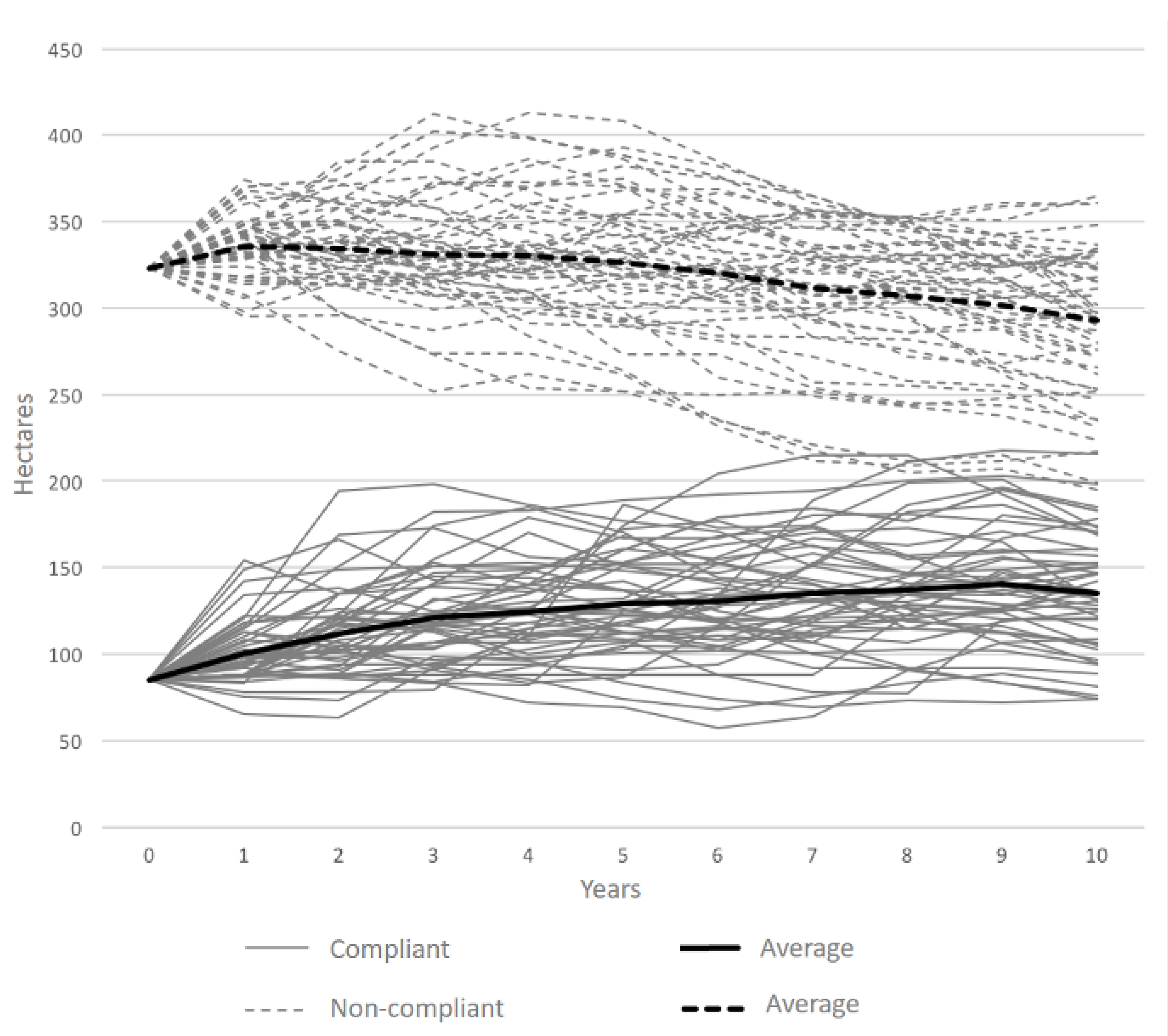
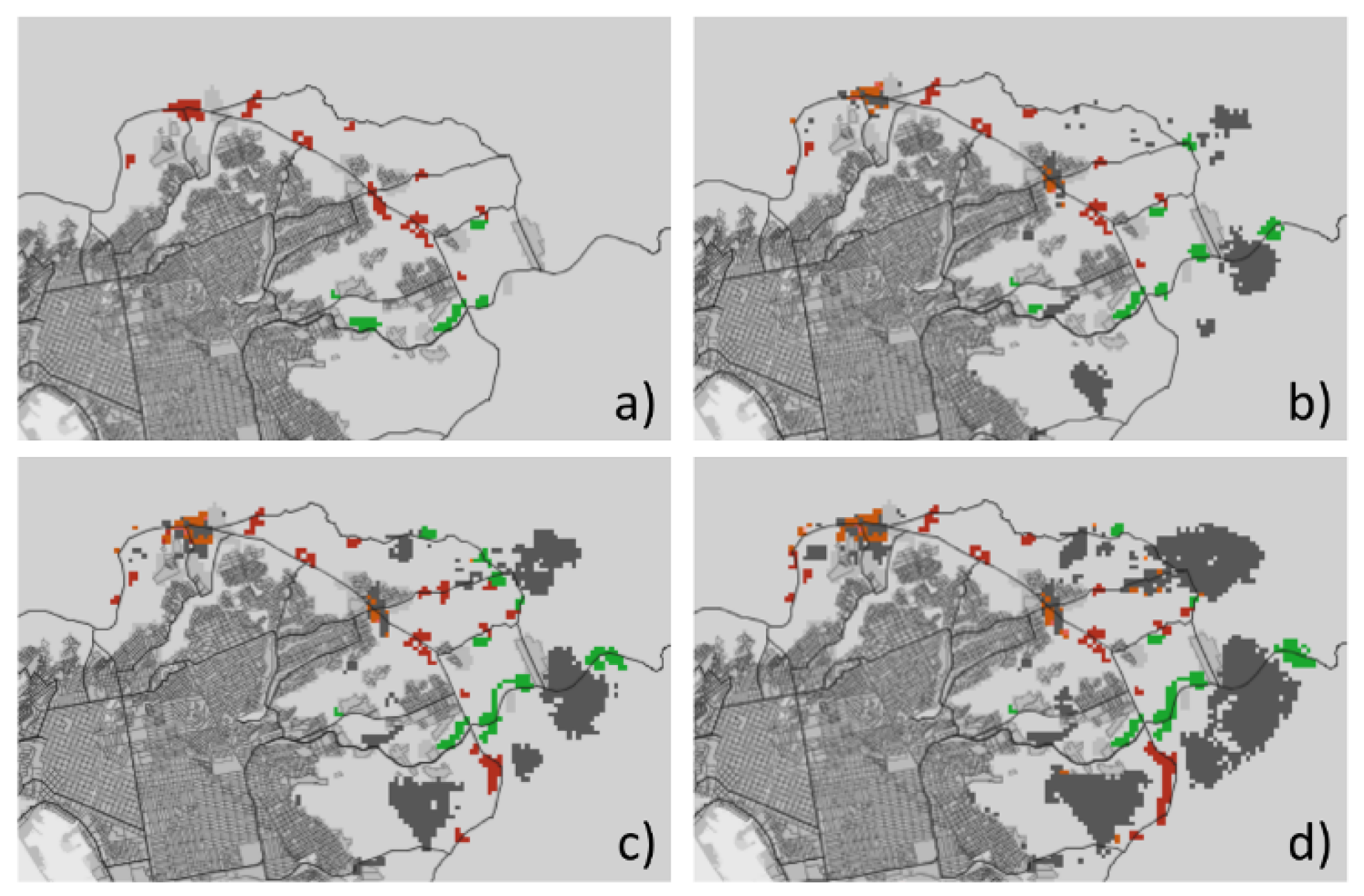
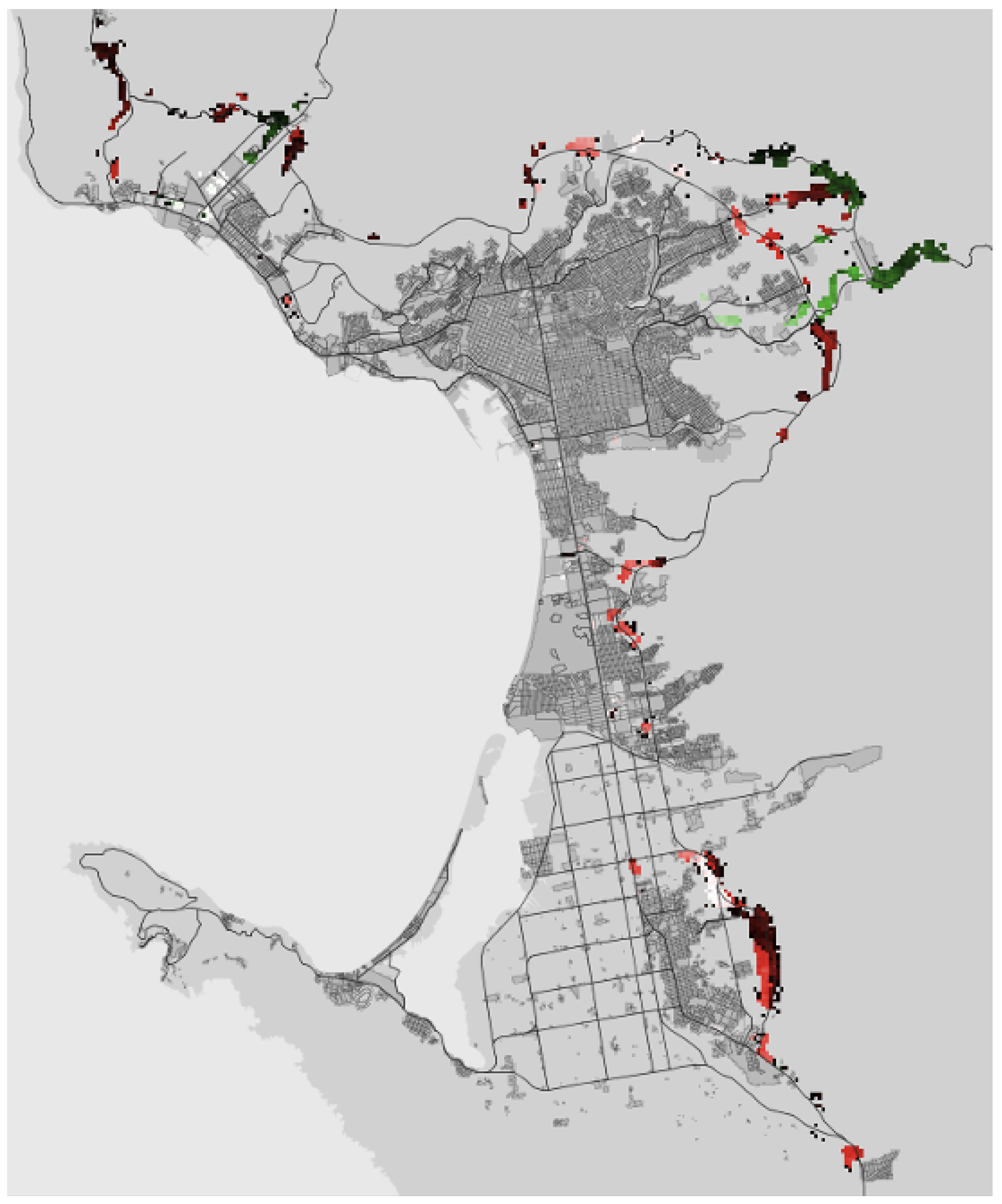
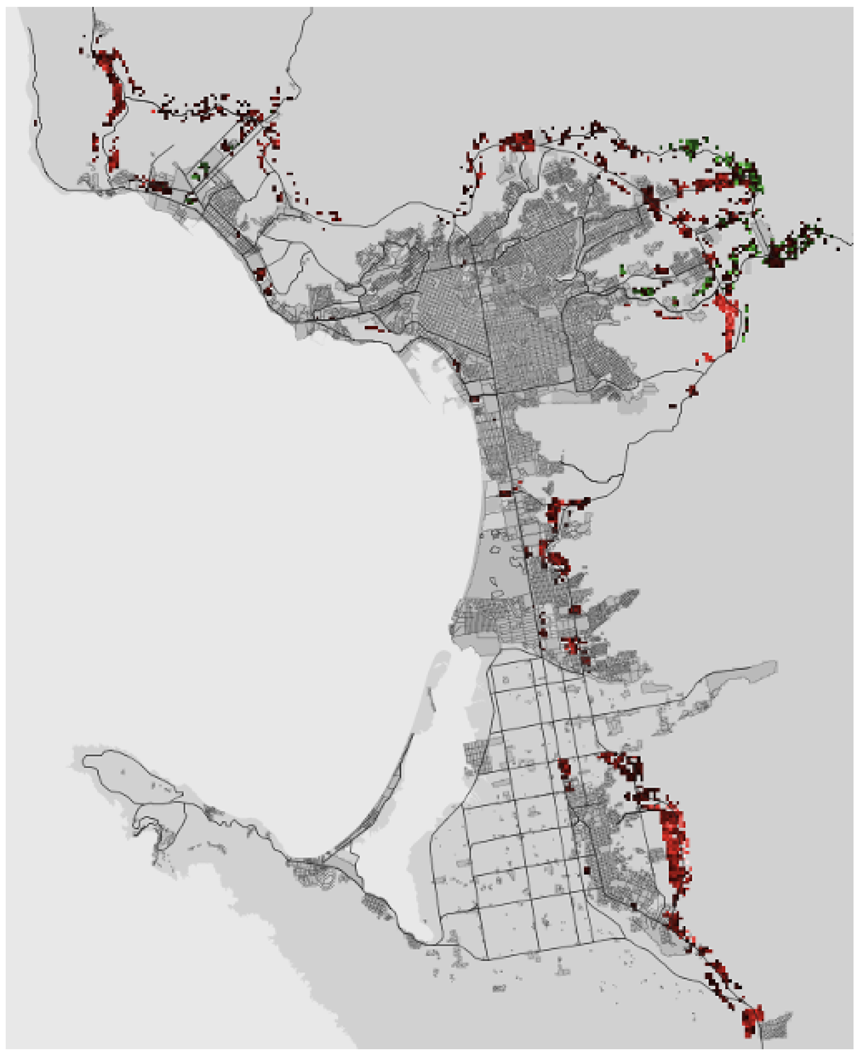
Total Attractive Land Footprint.	- There will always be more industry-attractive vacant land in normative incompatibility than in normative compatibility with thw UDPE. -The demand for industrial zoning is higher than the one established by the UDPE. - In low population densities secnarios between 10 to 20 inhabitants per hectare, Attractive Land drops steeply. - Emergence of an Attractive Land corridor along a regional road that communicates the northeast part of the city. - Low possibility of industry-attractive vacant land is occupied by this activity in almost all parts of the city, except two zones, but they regional roads are needed and are not compatible with UDPE regulations.
Percentage of urbanized Attractive Land Footprint.	- In low densities of 10 to 15 inhabitants per hectare, urbanization of Attractive Land Footprints tends to increase by up to 65%, compared to up to 14% when 35 inhabitants per hectare.
Urbanized Attractive Land Footprint differentiated by compatibility.	- Predominance of industry-attractive vacant land occupied by land-uses unrelated to this activity. - The most desirable scenario, industry-attractive vacant land occupied by industry and in accordance to UDPE regulations, was in last place in simulation results. - In low population density scenario between 10 to 20 inhabitants/ha, urbanization of industry-attractive vacant land rises rapidly, and occupied by non-industrial land uses. - In densities of approximately 40 Inhabitants/ha or higher, industrial surface outside of industry-attractive vacant land is low, which is a desired condition. - There is a moderate possibility of industry-attractive vacant land urbanization in most of the city’s northeastern sector. Northern and southern areas have the same possibility but is not allowed by the UDPE.
Urbanized attractive land footprint differentiated by land use.	- Residential land use mostly occupies industry-attractive vacant land, replicating current real-world competition between these two land uses.
Industry location differentiated by compatibility with the UDPE.	- In low densities between 10 to 25 hab/ha, the industrial surface in incompatible sub-sectors rises steeply over time. - There are zones with a high possibility of emerging industry-attractive vacant land but are incompatible with UDPE regulations, and a projected road network must be built first.
Attractive land footprint state.	- In low density scenarios, alive surface immediately goes down at the same rate that the dead surface rises. - In high density scenarios, dead surface rises at a faster rate than the surface that is alive. - Northeast corridor footprint: there is a high possibility of its urbanization by land uses other than industry.

Publisher’s Note: MDPI stays neutral with regard to jurisdictional claims in published maps and institutional affiliations.

© 2021 by the authors. Licensee MDPI, Basel, Switzerland. This article is an open access article distributed under the terms and conditions of the Creative Commons Attribution (CC BY) license (http://creativecommons.org/licenses/by/4.0/).

Share and Cite

MDPI and ACS Style

Sandoval-Félix, J.; Castañón-Puga, M.; Gaxiola-Pacheco, C.G. Analyzing Urban Public Policies of the City of Ensenada in Mexico Using an Attractive Land Footprint Agent-Based Model. Sustainability 2021, 13, 714. https://doi.org/10.3390/su13020714

AMA Style

Sandoval-Félix J, Castañón-Puga M, Gaxiola-Pacheco CG. Analyzing Urban Public Policies of the City of Ensenada in Mexico Using an Attractive Land Footprint Agent-Based Model. Sustainability. 2021; 13(2):714. https://doi.org/10.3390/su13020714

Chicago/Turabian Style

Sandoval-Félix, Javier, Manuel Castañón-Puga, and Carelia Guadalupe Gaxiola-Pacheco. 2021. "Analyzing Urban Public Policies of the City of Ensenada in Mexico Using an Attractive Land Footprint Agent-Based Model" Sustainability 13, no. 2: 714. https://doi.org/10.3390/su13020714

Note that from the first issue of 2016, this journal uses article numbers instead of page numbers. See further details here.

Article Menu

Analyzing Urban Public Policies of the City of Ensenada in Mexico Using an Attractive Land Footprint Agent-Based Model

Abstract

1. Introduction

2. Methodology

2.1. Data Requirements

2.2. Model Verification and Validation

2.2.1. Model Verification

2.2.2. Model Validation

2.2.3. Sample Space

2.3. Experiments

3. Simulation Results Analysis and Discussion

3.1. Total Attractive Land Footprint

3.2. Percentage of Urbanized Attractive Land Footprints

3.3. Urbanized Attractive Land Footprint Differentiated by Compatibility

3.4. Urbanized Attractive Land Footprint Differentiated by Land Use

3.5. Industry Location Differentiated by Compatibility with the UDPE

3.6. Attractive Land Footprint States

4. Conclusions

Supplementary Materials

Author Contributions

Funding

Institutional Review Board Statement

Informed Consent Statement

Data Availability Statement

Acknowledgments

Conflicts of Interest

Abbreviations

Appendix A. Complementary Tables and Figures

Appendix A.1. Attractive Factors by Land-Use Type

Appendix B. Modeling and Simulation Process

Appendix B.1. Data Requirements

Appendix B.2. Data Preparation

Appendix B.3. Land Use Compatibility Matrix

Appendix B.4. Spatial Data Layers

Appendix C. The Model

Appendix C.1. Overview, Design Concepts, and Details (ODD Protocol)

Overview

Purpose

Entities, State Variable and Scales

Process Overview and Scheduling

Appendix C.2. Design Concepts

Appendix C.2.1. Basic Principles

Emergence

Interaction

Stochasticity

Collectives

Observation

Appendix C.2.2. Details

Attractive Land

Initialization

Input Data

Sub-Models

References

Share and Cite

Article Metrics

Article Access Statistics

Further Information

Guidelines

MDPI Initiatives

Follow MDPI