An Optimization Model for Water Management under the Dual Constraints of Water Pollution and Water Scarcity in the Fenhe River Basin, North China

Abstract

Sustainable watershed development suffers from severe challenges, such as water pollution and water scarcity. Based on an analysis of water quality and water utilization in the Fenhe River Basin, an inexact two-stage stochastic programming model with downside-risk aversion was built for optimal water resource allocations for the four primary water use sectors (industry, domestic use, agriculture, and the environment) in the Fenhe River Basin. The model aims to maximize the comprehensive watershed benefits, including water benefits, water costs, water treatment costs, and downside risks. The constraints are water quality, available water resources, and sectoral demands in different hydrological scenarios. The results show that pollutant emissions decrease as risk-aversion levels increase and show the opposite trend in the midstream and downstream areas. The increase in water resource allocation for agriculture and reduction in ecological water indicate that agriculture suffered the greatest water shortage and risk. Improving water recycling and coordinating the transferred water resources increases the comprehensive benefits and reduces sectoral risks. The model effectively manages rational water allocations under dual constraints and provides support for coordinating socio-economic development and environmental protection in the river basin.

1. Introduction

Water resources play a central role in human survival, ecosystem security, and socio-economic development [1,2,3]. However, with the rapid population expansion and economic development, water shortages and water pollution have become severe problems worldwide [4,5,6]. Excessive water resource exploitation, inefficient utilization, and increased pollutant emissions have exacerbated the deterioration of water quality and water scarcity [7,8]. Water pollution is the most pressing issue in China, and water scarcity has become a critical constraint for regional socio-economic development [9,10]. High-quality and sustainable development based on improving water quality and rational water resource utilization is a developmental priority in China. Therefore, optimal regional and sectoral water resource allocation for coordinated development between the social economy and the environment are important.

Previous studies reveal that optimal allocation of water resources is one of the most effective resolutions for addressing water pollution, water shortages, and rising water demand [11,12,13,14,15,16]. Moreover, appropriate policy interventions, such as adjusting the industrial structure and technological progress, are necessary to achieve harmonious economic and societal development [17]. Additionally, there are many uncertainties in the water environment system, including stochasticity of available water resources caused by climate change [18,19,20,21], uncertainties regarding plans and policies, and the complexity of interconnected processes between the social economy and the environment (e.g., water utilization, wastewater treatment, recycling, and water quality). These uncertainties generate enormous challenges for water resources and water quality management.

Several optimization approaches have been developed for water resource allocation and water quality management with uncertainties [22,23,24,25,26]. The inexact two-stage stochastic programming (ITSP) model, which integrates interval-parameter programming (IPP) and two-stage stochastic programming (TSP), has been widely applied to address different forms of multiple uncertainties in water resource allocation and water quality management [27,28,29,30,31,32]. However, the ITSP model does not consider the variability of the second-stage cost or benefit, which may lead to an unbalanced allocation pattern [33,34]. Previous studies have found that the downside-risk method is an advantageous measure that balances benefits and resource allocation by minimizing the risks for all parties under certain conditions [35]. The downside risk method can be integrated with the programming model with a scenario-based description of problem data and generate a series of solutions that help decision-makers quantitatively evaluate trade-offs between the system’s economy and stability [36,37,38]. Moreover, most studies do not sufficiently consider watersheds with severe water pollution and water scarcity problems, such as the Fenhe River basin in the Shanxi province, northern China. The Fenhe River increasingly suffers from environmental problems, such as severe water pollution and ecological damage, which exacerbates watershed water shortages and cross-sectoral water competition [39]. Thus, an effective approach for dealing with severe environmental problems and water shortages in river basins must be explored.

Therefore, this study aims to develop an ITSP model and introduce downside-risk aversion (ITSDP) to address rational water resource allocation under the dual constraints of water pollution and water shortage in the Fenhe River Basin. The model combines comprehensive water benefits with environmental protection, as the water resource conflict between the environment and production sectors must be resolved, and water resource allocation strategies for different watershed divisions and sectors should be optimized to ensure coordinated development. Figure 1 presents the general framework of the ITSDP model for optimal water management in the Fenhe River Basin with uncertainties for integrating water quality management and water resource allocation. The application of the model could help optimize regional water resource allocation strategies and pollutant emissions under the constraints of water quality and water quantities. Furthermore, the results could help watershed decision-makers establish and improve water-based industrial structures and layouts.

2. Materials and Methods

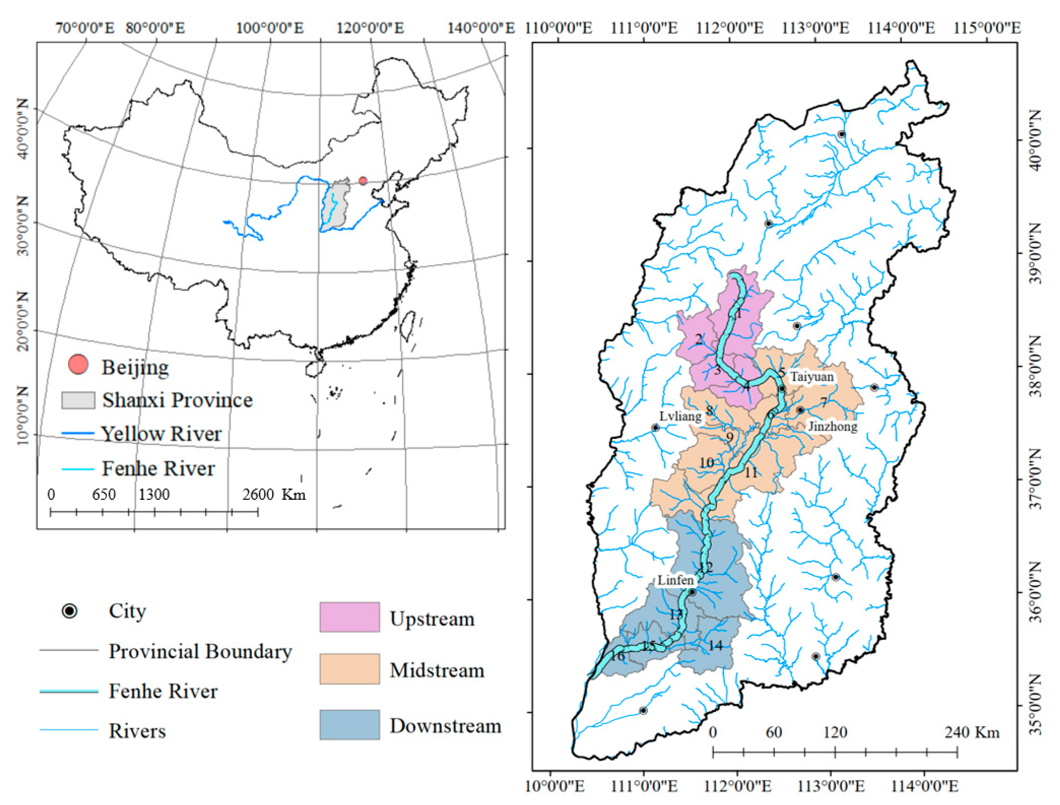
2.1. Study Area

The Fenhe River (110°30′ E–113°32′ E, 35°20′ N–39°00′ N) is the second largest branch of the Yellow River and the largest river in Shanxi, with a total length of 694 km and a watershed area of approximately 39,471 km² [40]. The Fenhe River Basin has a semi-humid climate, the multi-year (1956–2010) average rainfall of the entire basin is 504.8 mm (with a ten-year decreasing trend), and the water surface evaporation is 900–1200 mm. The total available water resources (from 1956–2010) of the Fenhe River Basin are 2.656 billion m³ [41].

The Fenhe River Basin is highly urbanized and agriculturally developed. The utilization of surface water development is over 70%, and the average utilization of groundwater development reaches 85% [42]. However, the Fenhe River Basin is a relatively severely water-deprived region with a water resource per capita of 378 m³—18% of the national average [40]. The utilization rate of water resources has long exceeded 70%, leading to severe water conflicts between the social economy and the environment [42]. Moreover, due to over-exploitation, uneven allocation, and low utilization efficiency of water resources, excessive pollutant discharge has caused severe environmental problems in the Fenhe River.

In this study, the scope of the Fenhe River Basin was determined by analysis of data from a Digital Elevation Model in theShanxi province, using the hydrological analysis module of ARCGIS. The river basin is divided into the upstream, midstream, and downstream areas and a total of 16 water environment control units with the corresponding water quality sections (Figure 2).

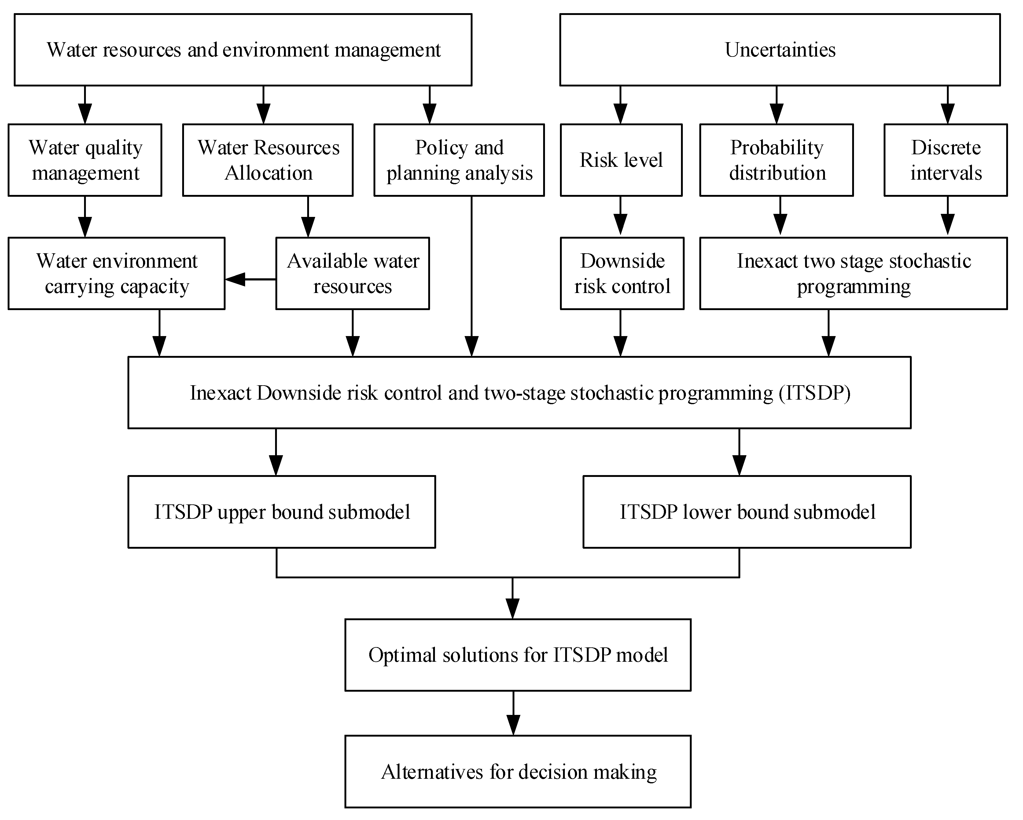
2.2. Model Development

This study considers long-run programming of 15 years and three periods (i.e., 2021–2025, 2026–2030, and 2031–2035). Three hydrological scenarios (low, medium, and high) reflect different water environment carrying capacities and water resources. The ITSDP model for integrating water benefits and downside-risk control under dual constraints of water shortage and pollution in the Fenhe River Basin was formulated as follows:

$$max{f}^{\pm }=f_1^{\pm }-f_2^{\pm }-f_3^{\pm }-f_4^{\pm }-f_5^{\pm }-f_6^{\pm }$$

(1)

where $f^{\pm }$ is the comprehensive benefit of the basin (10⁶ million CNY) over the programming periods.

• Water utilization benefits:

$$f_1^{\pm }={\displaystyle \sum _{i=1}^{16}{\displaystyle \sum _{k=1}^4{\displaystyle \sum _{t=1}^3{L}_t\cdot UN{B}_{ikt}^{\pm }\cdot \left(IA{W}_{ikt}^{\pm }+{\displaystyle \sum _{h=1}^3{p}_h\cdot R{W}_{ikth}^{\pm }}\right)}}}$$

(2)

where $i$ denotes the control unit; $k$ denotes the water sectors ($k$ = 1 for industry, $k$ = 2 for domestic, $k$ = 3 for agriculture, and $k$ = 4 for the environment); t denotes different periods; $L_t$ denotes the length of period t, and the values are fixed at 5 years; $UN{B}_{ikt}^{\pm }$ represents the sectoral water-use benefit (10⁴ CNY/10⁴ m³); represents the pre-allocation of water resources for each sector (10⁴ m³/year); and $R{W}_{jkt}^{\pm }$ represents reused water resources for each sector (10⁴ m³/year).

2.

Water shortage penalty:

$$f_2^{\pm }={\displaystyle \sum _{i=1}^{16}{\displaystyle \sum _{k=1}^4{\displaystyle \sum _{t=1}^3{\displaystyle \sum _{h=1}^3{L}_t\cdot p_h\cdot PN{B}_{ikt}^{\pm }\cdot D{W}_{ikth}^{\pm }}}}}$$

(3)

where h denotes hydrological scenarios, $p_h$ denotes the occurrence probability of scenario h, $PN{B}_{jkt}^{\pm }$ represents the reduction of net benefit per unit of water resource not delivered (10⁴ RMB/10⁴ m³), and $D{W}_{ikth}^{\pm }$ represents the allocation deficit of water resources for each sector (10⁴ m³/year).

3.

Cost of water supply:

$$\begin{array}{ll}{f}_3^{\pm }=& {\displaystyle \sum _{i=1}^{16}{\displaystyle \sum _{k=1}^4{\displaystyle \sum _{t=1}^3{L}_t\cdot \left(IA{W}_{ikt}^{\pm }-{\displaystyle \sum _{h=1}^3{p}_h\cdot D{W}_{ikth}^{\pm }}\right)\cdot C{W}_{ikt}^{\pm }}}}\\ & +{\displaystyle \sum _{i=1}^{16}{\displaystyle \sum _{k=1}^4{\displaystyle \sum _{t=1}^4{\displaystyle \sum _{h=1}^3{p}_h\cdot L_t\cdot R{W}_{ikth}^{\pm }\cdot CR{W}_{ikt}^{\pm }}}}}\end{array}$$

(4)

where $C{W}_{jkt}^{\pm }$ represents the cost of the water supplies (10⁴ CNY/10⁴ m³) and $CR{W}_{jkt}^{\pm }$ is the cost of reused water (10⁴ CNY/10⁴ m³).

4.

Cost of wastewater treatment:

$$f_4^{\pm }={\displaystyle \sum _{i=1}^{16}{\displaystyle \sum _{k=1}^4{\displaystyle \sum _{t=1}^3{L}_t\cdot \left(IA{W}_{ikt}^{\pm }-{\displaystyle \sum _{h=1}^3{p}_h\cdot D{W}_{ikth}^{\pm }}\right)\cdot {\alpha }_{ikt}^{\pm }\cdot \left(CW{W}_{ikt}^{\pm }+{\xi }_{ikt}^{\pm }\cdot CRW{T}_{ikt}^{\pm }\right)}}}$$

(5)

where $CW{W}_{jkt}^{\pm }$ represents the costs of wastewater treatment (10⁴ CNY/10⁴ m³) and $\mathit{CRW}{T}_{jkt}^{\pm }$ denotes the costs of wastewater reclamation (10⁴ CNY/10⁴ m³).

5.

Cost of ecological water:

$$f_5^{\pm }={\displaystyle \sum _{i=1}^{16}{\displaystyle \sum _{t=1}^3{\displaystyle \sum _{h=1}^3{L}_t\cdot p_h\cdot G{W}_{ith}^{\pm }\cdot CE{W}_{it}^{\pm }}}}$$

(6)

where $G{W}_{ith}^{\pm }$ is the ecological water (i.e., ecological water is to purify excessive pollutant emission) and $CE{W}_{it}^{\pm }$ is the cost of ecological water.

6.

Downside risk constraints:

$$f_6^{\pm }=\omega \cdot {\displaystyle \sum _{i=1}^{16}{\displaystyle \sum _{k=1}^4{\displaystyle \sum _{t=1}^{3}DRis{k}_{ikt}^{\pm }}}}$$

(7)

where $\omega$ represents the risk control level and $DRis{k}_{ikt}^{\pm }$ is the sectoral downside risk.

Constraints:

• Water resource constraints:

$${\displaystyle \sum _{k=1}^4\left(IA{W}_{ijkt}^{\pm }-D{W}_{ijkth}^{\pm }\right)}\le AW{Q}_{it}^{\pm };\forall i,t,h$$

(8)

$${\displaystyle \sum _{i=1}^{16}{\displaystyle \sum _{k=1}^4\left(IA{W}_{ikt}^{\pm }-D{W}_{ikth}^{\pm }\right)}+G{W}_{ith}^{\pm }}\le TAW{Q}_t^{\pm };\forall t,h$$

(9)

$$DIA{W}_{ikth}^{\pm }\le IA{W}_{ikt}^{\pm };\forall i,k,t,h$$

(10)

where $AW{Q}_{it}^{\pm }$ denotes the available regional water resources (10⁴ m³/year).

2.

Water sector demand constraints:

$$\left(IA{W}_{ikt}^{\pm }-D{W}_{ikth}^{\pm }\right)+R{W}_{ikth}^{\pm }\ge W{D}_{\min ikt}^{\pm };\forall i,k,t,h$$

(11)

$$\left(IA{W}_{ikt}^{\pm }-D{W}_{ikth}^{\pm }\right)+R{W}_{ikth}^{\pm }\le W{D}_{\max ikt}^{\pm };\forall i,k,t,h$$

(12)

where $W{D}_{\min ikt}^{\pm }$ represents the minimum water resources requirement and $W{D}_{\max ikt}^{\pm }$ represents the maximum water resources requirement (10⁴ m³/year).

3.

Regional wastewater treatment capacity constraints:

$${\displaystyle \sum _{j=1}^3\left(IA{W}_{ijkt}^{\pm }-D{W}_{ijkth}^{\pm }\right)}\cdot {\alpha }_{ikt}^{\pm }\le AT{W}_{ikt}^{\pm },\forall i,t,h,k=1,2$$

(13)

where ${\alpha }_{ikt}$ is the wastewater emission coefficient and $AT{W}_{ikt}^{\pm }$ represents the wastewater treatment capacity (10⁴ tons).

4.

Regional wastewater reuse capacity constraints:

$$\left(IA{W}_{ikt}^{\pm }-D{W}_{ikth}^{\pm }\right)\cdot {\alpha }_{ikt}^{\pm }\cdot {\xi }_{ikt}^{\pm }\ge {\displaystyle \sum _{k=1}^{4}R{W}_{ikth}^{\pm }},\forall i,t,h$$

(14)

where ${\xi }_{jkt}$ is the wastewater reuse rate.

5.

Water environment carrying capacity constraints:

$$\begin{array}{l}{\displaystyle \sum _{k=1}^3{\displaystyle \sum _{j=1}^3\left(IA{W}_{ijkt}^{\pm }-DIA{W}_{ijkth}^{\pm }\right)}\cdot {\alpha }_{ikt}^{\pm }\cdot \left(1-{\xi }_{ikt}^{\pm }\right)\cdot E{C}_{krt}^{\pm }\cdot ID{R}_{krt}}\\ -\left(C{S}_{irt}^{\pm }-C{0}_{irt}^{\pm }\right)\cdot G{W}_{ith}^{\pm }\le AL{D}_{irth}^{\pm },\forall i,r,t,h\end{array}$$

(15)

where r is the controlled water pollutant (r = 1 for chemical oxygen demand (COD), r = 2 for ammonia nitrogen (NH₄-N), r = 3 for total phosphorus (TP)), $E{C}_{ikrt}^{\pm }$ represents the concentration of pollutants after wastewater treatment (mg/L), $ID{R}_{krt}$ represents the river load ratio of different pollutants, and $AL{D}_{irth}^{\pm }$ is the environmental capacity (tons) of different pollutants.

6.

Downside risk

$$PR{W}_{ikth}^{\pm }=L_t\cdot \left\{\begin{array}{l}UN{B}_{ikt}^{\pm }\cdot \left(IA{W}_{ikt}^{\pm }+R{W}_{ikth}^{\pm }\right)-PN{B}_{ikt}^{\pm }\cdot D{W}_{ikth}^{\pm }\\ -\left[\left(IA{W}_{ikt}^{\pm }-D{W}_{ikth}^{\pm }\right)\cdot C{W}_{ikt}^{\pm }+R{W}_{ikth}^{\pm }\cdot CR{W}_{ikt}^{\pm }\right]\\ -\left(IA{W}_{ikt}^{\pm }-D{W}_{ikth}^{\pm }\right)\cdot \left({\alpha }_{ikt}^{\pm }\cdot CW{W}_{ikt}^{\pm }+{\alpha }_{ikt}^{\pm }\cdot {\xi }_{ikt}^{\pm }\cdot CRW{T}_{ikt}^{\pm }\right)\end{array}\right\},\forall i,k,t,h$$

(16)

$$Delt{a}_{ikth}^{\pm }=\{\begin{array}{ll}{\mathsf{\Omega }}_{it}^{\pm }-PR{W}_{ikth}^{\pm },& PR{W}_{ikth}^{\pm }<{\mathsf{\Omega }}_{ikt}^{\pm }\\ 0,& PR{W}_{ikth}^{\pm }>{\mathsf{\Omega }}_{ikt}^{\pm }\end{array},\forall i,k,t,h$$

(17)

$$DRis{k}_{ikt}^{\pm }={\displaystyle \sum _{h=1}^3{p}_h\cdot Delt{a}_{ikth}^{\pm }},\forall i,k,t$$

(18)

where $PR{W}_{ikth}^{\pm }$ represents the actual benefit, ${\mathsf{\Omega }}_{ikt}^{\pm }$ represents the expected regional benefit, $Delt{a}_{ikth}^{\pm }$ represents the positive deviation from the expected benefit, and $DRis{k}_{ikt}^{\pm }$ represents the downside risk.

The objective is to maximize the comprehensive benefits of the river basin, including the benefits of water resource sectors, water shortage penalties, and the cost of water supply, wastewater treatment, and wastewater reclamation. The constraints are for the relationships between decision values and water quality requirements, including available water resources, environmental water carrying capacity, and downside risks.

Using an interactive algorithm, the ITSDP model can be transformed into two deterministic sub-models that correspond to the lower and upper bounds of the desired objective function value. The $D{W}_{ikth}^{-}$, $R{W}_{ikth}^{+}$, $G{W}_{ith}^{-}$, $DRis{k}_{ikt}^{-}$ and $D{W}_{ikth}^{+}$, $R{W}_{ikth}^{-}$, $G{W}_{ith}^{+}$, $DRis{k}_{ikt}^{+}$ sub-models are solved to form the final ITSDP model solution: [$DIA{W}_{ikth}^{-}$, $DIA{W}_{ikth}^{+}$], [$R{W}_{ikth}^{-}$, $R{W}_{ikth}^{+}$], [$G{W}_{ith}^{-}$, $G{W}_{ith}^{+}$], and [$DRis{k}_{ikt}^{-}$, $DRis{k}_{ikt}^{+}$].

2.3. Datasets

Table 1. Available water resources in the Fenhe River Basin (10⁴ m³/year).

Water Resources	Periods	Regions
		Upstream	Midstream	Downstream
Surface water	t = 1	[22,640, 28,300]	[59,200, 74,000]	[27,840, 34,800]
	t = 2	[22,880, 28,600]	[61,520, 76,900]	[27,840, 34,800]
	t = 3	[23,120, 28,900]	[63,840, 79,800]	[27,840, 34,800]
Groundwater	t = 1	[2560, 3200]	[49,600, 62,000]	[24,600, 30,750]
	t = 2	[2560, 3200]	[47,120, 58,900]	[22,880, 28,600]
	t = 3	[2560, 3200]	[44,640, 55,800]	[21,160, 26,450]
Transferred water	t = 1	[1800, 2250]	[76,800, 96,000]	[54,840, 68,550]
	t = 2	[2400, 3000]	[86,400, 108,000]	[59,920, 74,900]
	t = 3	[3000, 3750]	[96,000, 120,000]	[65,000, 81,250]

lists the available water resources in the upper, middle, and lower reaches of the Fenhe River, including surface water, groundwater, and transferred water from the Yellow River. These were calculated based on regional water resource planning and management policies.

Table 2. Water environment carrying capacities in the Fenhe River Basin (tons).

Periods	Pollutants	Regions	Hydrological Scenarios
			h = 1	h = 2	h = 3
t = 1	r = 1	upstream	1297.46	1996.10	3629.27
		midstream	13,888.68	21,367.20	38,849.45
		downstream	6375.08	9807.82	17,832.40
	r = 2	upstream	90.62	139.42	253.49
		midstream	345.84	532.06	967.38
		downstream	65.81	101.24	184.08
	r = 3	upstream	32.55	50.07	91.04
		midstream	210.06	323.18	587.59
		downstream	57.26	88.09	160.16
t = 2	r = 1	upstream	1297.46	1996.10	3629.27
		midstream	13,390.74	20,601.13	37,456.61
		downstream	4781.31	7355.87	13,374.30
	r = 2	upstream	90.62	139.42	253.49
		midstream	343.55	528.53	960.97
		downstream	49.36	75.93	138.06
	r = 3	upstream	32.55	50.07	91.04
		midstream	207.15	318.70	579.45
		downstream	42.94	66.07	120.12
t = 3	r = 1	upstream	1297.46	1996.10	3629.27
		midstream	10,805.19	16,623.37	29,110.03
		downstream	4781.31	7355.87	9807.82
	r = 2	upstream	90.62	139.42	253.49
		midstream	303.03	466.19	842.50
		downstream	49.36	75.93	101.24
	r = 3	upstream	32.55	50.07	91.04
		midstream	176.33	271.28	486.72
		downstream	42.94	66.07	88.09

lists the water environment carrying capacities in the Fenhe River Basin, which were calculated based on hydrological parameters under different scenarios.

3. Results and Discussions

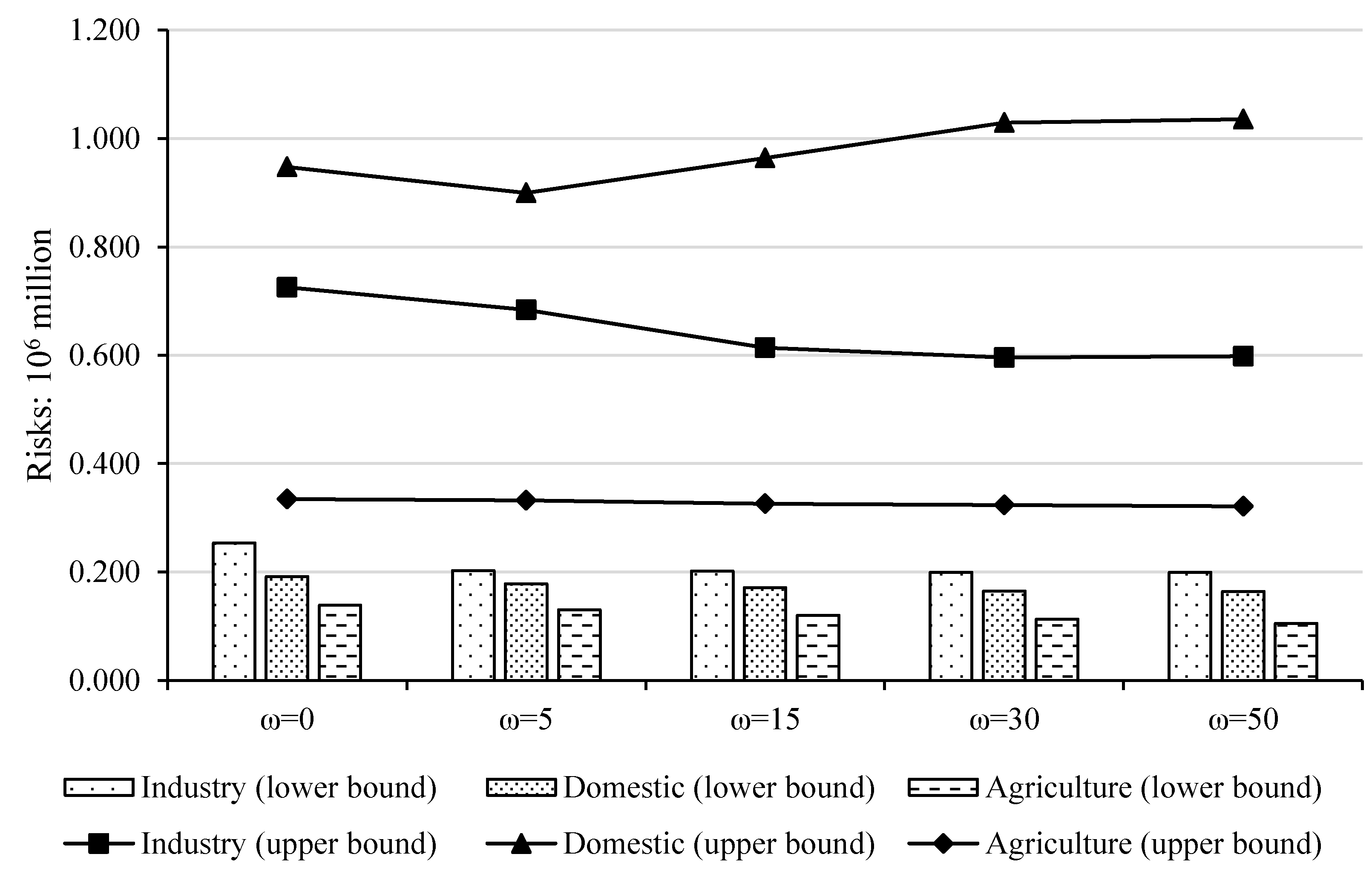
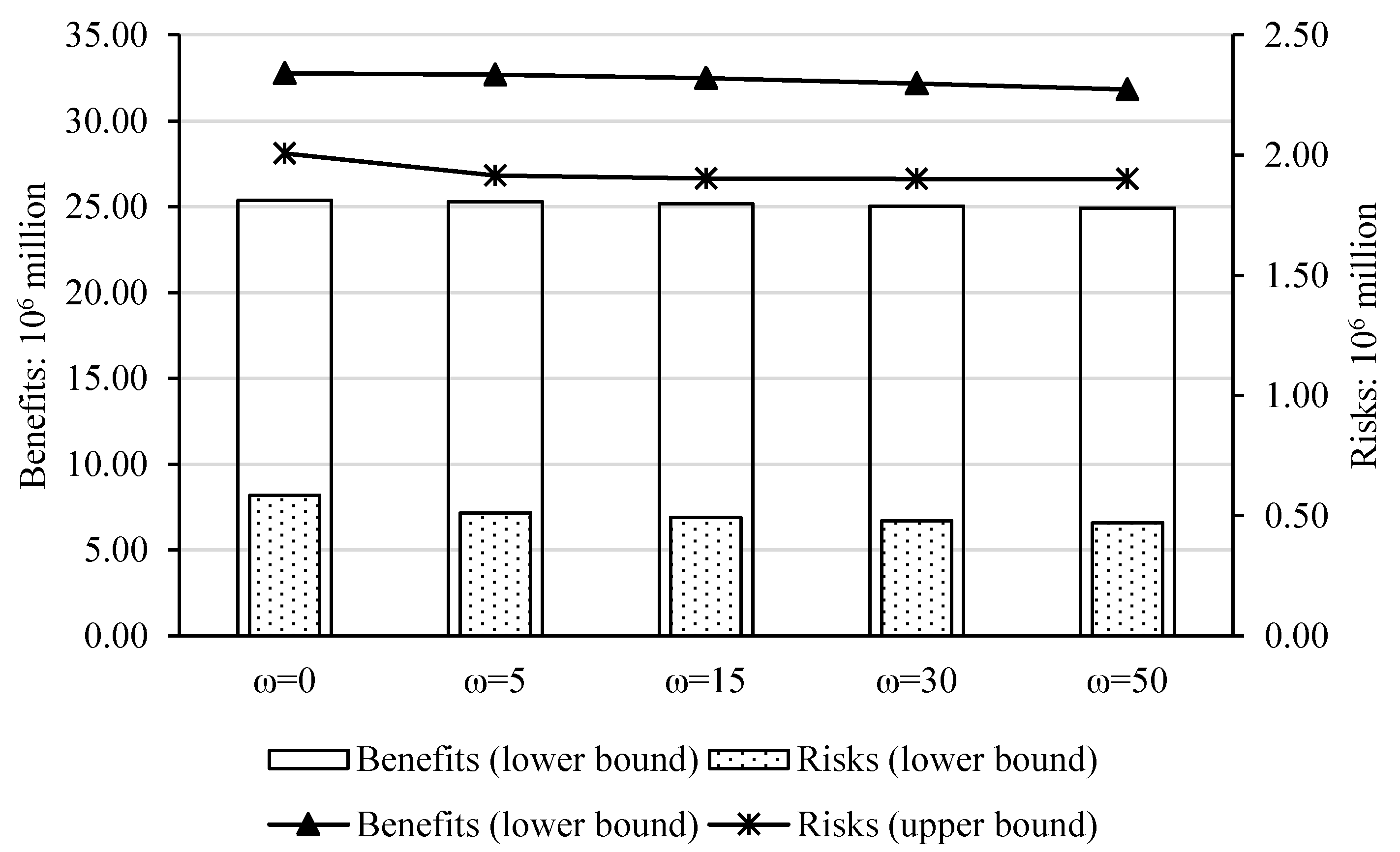
3.1. System Benefits and Risks

In this study, the optimal results were obtained without the downside-risk control constraints for a $\omega$ value fixed at 0. Further, values of 5, 15, 30, and 50 were selected to reflect increasing risk control levels and obtain the corresponding optimal results of water resource allocation and pollutant emissions. In this section, we compare and analyze the differences in the system benefits and risks of the Fenhe River Basin under different risk levels.

Figure 3 shows the system benefits of water resource utilization and corresponding risks for different $\omega$ values. The figure shows a similar change in benefits and risks. The total benefits are CNY [25.39, 32.76], [25.29, 32.68], [25.18, 32.47], [25.04, 32.15], and [24.92, 31.81] × 10⁶ million, and the risks are [0.58, 2.01], [0.51, 1.92], [0.49, 1.90], [0.48, 1.90], and [0.47, 1.90] × 10⁶ million for $\omega$ of 0, 5, 15, 30, and 50, respectively. Both benefits and risks decrease slightly as the $\omega$ values increase, indicating that certain water resources transfer to lower-benefit sectors to meet the stronger risk-control requirement. As the risk control level increases, the model will optimize the water resource allocations for units and sectors based on factors such as water efficiencies, pollutant emission intensities, and water environment carrying capacities.

Figure 4 shows different changes in sectoral risks. Industry and agriculture risks show a downward trend as risk control levels increase, and the risks are CNY [0.253, 0.725], [0.202, 0.684], [0.202, 0.614], [0.200, 0.596], and [0.199, 0.598] × 10⁶ million and CNY [0.139, 0.335], [0.130, 0.332], [0.120, 0.326], [0.113, 0.323], and [0.105, 0.321] × 10⁶ million, for values of 0, 5, 15, 30, and 50, respectively. However, domestic risks are CNY [0.192, 0.947], [0.178, 0.900], [0.171, 0.964], [0.165, 1.029], and [0.164, 1.035] × 10⁶ million, respectively. The upper bound of the risks gradually increases for values of 5, 15, 30, and 50. These risks correspond to the lower bound of water resources and environmental carrying capacity, and more water resources are allocated to sectors with high benefits and low pollutant emission intensities.

Table 3. Sectoral risks in the Fenhe River Basin (CNY 10⁶ million).

Periods	Sectors	Regions	Risk Control Levels
			ω = 0	ω = 5	ω = 15	ω = 30	ω = 50
t = 1	Industry	upstream	0	0	0	0	0
		midstream	0	0	0	0	0
		downstream	[0, 0.007]	0	0	0	0
	Domestic	upstream	0	0	0	0	0
		midstream	[0.032, 0.045]	[0.031, 0.045]	[0.031, 0.044]	[0.031, 0.045]	[0.031, 0.045]
		downstream	0	0	0	0	0
	Agriculture	upstream	[0.001, 0.003]	[0.001, 0.002]	[0.001, 0.002]	[0.001, 0.002]	[0.001, 0.002]
		midstream	[0.005, 0.027]	[0.005, 0.027]	[0.005, 0.025]	[0.005, 0.025]	[0.005, 0.024]
		downstream	[0.019, 0.046]	[0.018, 0.045]	[0.018, 0.045]	[0.017, 0.045]	[0.015, 0.044]
t = 2	Industry	upstream	0	0	0	0	0
		midstream	0	0	0	0	0
		downstream	[0, 0.157]	[0, 0.124]	[0, 0.124]	[0, 0.124]	[0, 0.124]
	Domestic	upstream	0	0	0	0	0
		midstream	[0.019, 0.049]	[0.016, 0.048]	[0.016, 0.048]	[0.015, 0.052]	[0.015, 0.052]
		downstream	0	0	0	0	0
	Agriculture	upstream	[0.001, 0.004]	[0.001, 0.004]	[0.001, 0.004]	[0.001, 0.004]	[0.001, 0.004]
		midstream	[0.006, 0.037]	[0.006, 0.038]	[0.006, 0.034]	[0.006, 0.034]	[0.006, 0.033]
		downstream	[0.03, 0.059]	[0.029, 0.059]	[0.029, 0.059]	[0.028, 0.058]	[0.026, 0.058]
t = 3	Industry	upstream	[0, 0.006]	[0,0.005]	[0,0.004]	[0,0.004]	[0,0.006]
		midstream	[0, 0.012]	[0,0.012]	[0,0.012]	[0,0.012]	[0,0.012]
		downstream	[0.253, 0.543]	[0.202, 0.543]	[0.202, 0.474]	[0.200, 0.456]	[0.199, 0.456]
	Domestic	upstream	0	0	0	0	0
		midstream	[0.013, 0.371]	[0.006, 0.345]	[0.006, 0.337]	[0.004, 0.352]	[0.004, 0.356]
		downstream	[0.128, 0.482]	[0.125, 0.461]	[0.119, 0.535]	[0.115, 0.580]	[0.115, 0.582]
	Agriculture	upstream	[0.002, 0.005]	[0.002, 0.005]	[0.002, 0.005]	[0.001, 0.005]	[0.001, 0.005]
		midstream	[0.034, 0.079]	[0.027, 0.078]	[0.02, 0.078]	[0.018, 0.078]	[0.016, 0.078]
		downstream	[0.041, 0.074]	[0.040, 0.074]	[0.038, 0.073]	[0.036, 0.072]	[0.035, 0.072]

lists the sectoral risks in different periods and regions. The results show trends consistent with the analysis on total risks in the river basin. For example, in period 3, industry and agriculture risks in the downstream area are CNY [0.253, 0.543], [0.202, 0.543], [0.202, 0.474], [0.200, 0.456], and [0.199, 0.456] × 10⁶ million and CNY [0.041, 0.074], [0.040, 0.074], [0.038, 0.073], [0.036, 0.072], and [0.035, 0.072] × 10⁶ million, showing a downward trend as the $\omega$ values increase. Domestic risks show an upward trend for $\omega$ values of 5, 15, 30, and 50, and the risks are CNY [0.125, 0.461], [0.119, 0.535], [0.115, 0.580], and [0.115, 0.582]. In period 1, the agriculture risks in the upstream area are CNY [0.001, 0.003], [0.001, 0.002], [0.001, 0.002], [0.001, 0.002], and [0.001, 0.002] × 10⁶ million, and the risks remain unchanged for values of 5, 15, 30, and 50. The industry and domestic risks are zero, indicating that the system’s benefits and risks are balanced. Compared to the other areas, the upstream area has relatively sufficient water resources and environmental carrying capacity. The developed ITSDP model can optimize water resource allocation strategies to meet the highest system benefit under different risk control requirements. Furthermore, the supply of ecological water resources to purify water quality reduces the amount of water available for production and increases risks. The strong water quality constraint plays a decisive role in the optimal allocation of water resources in this study.

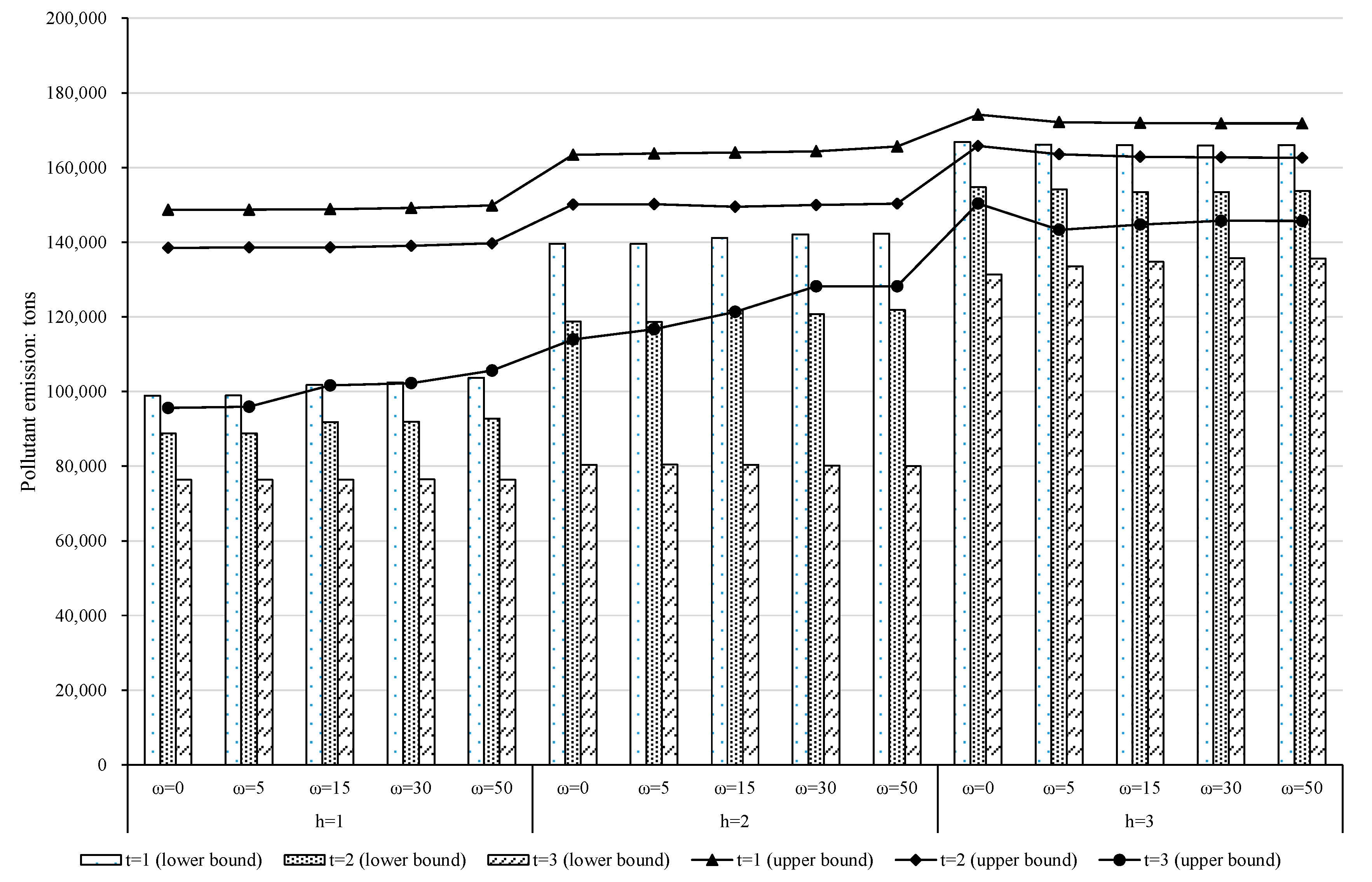
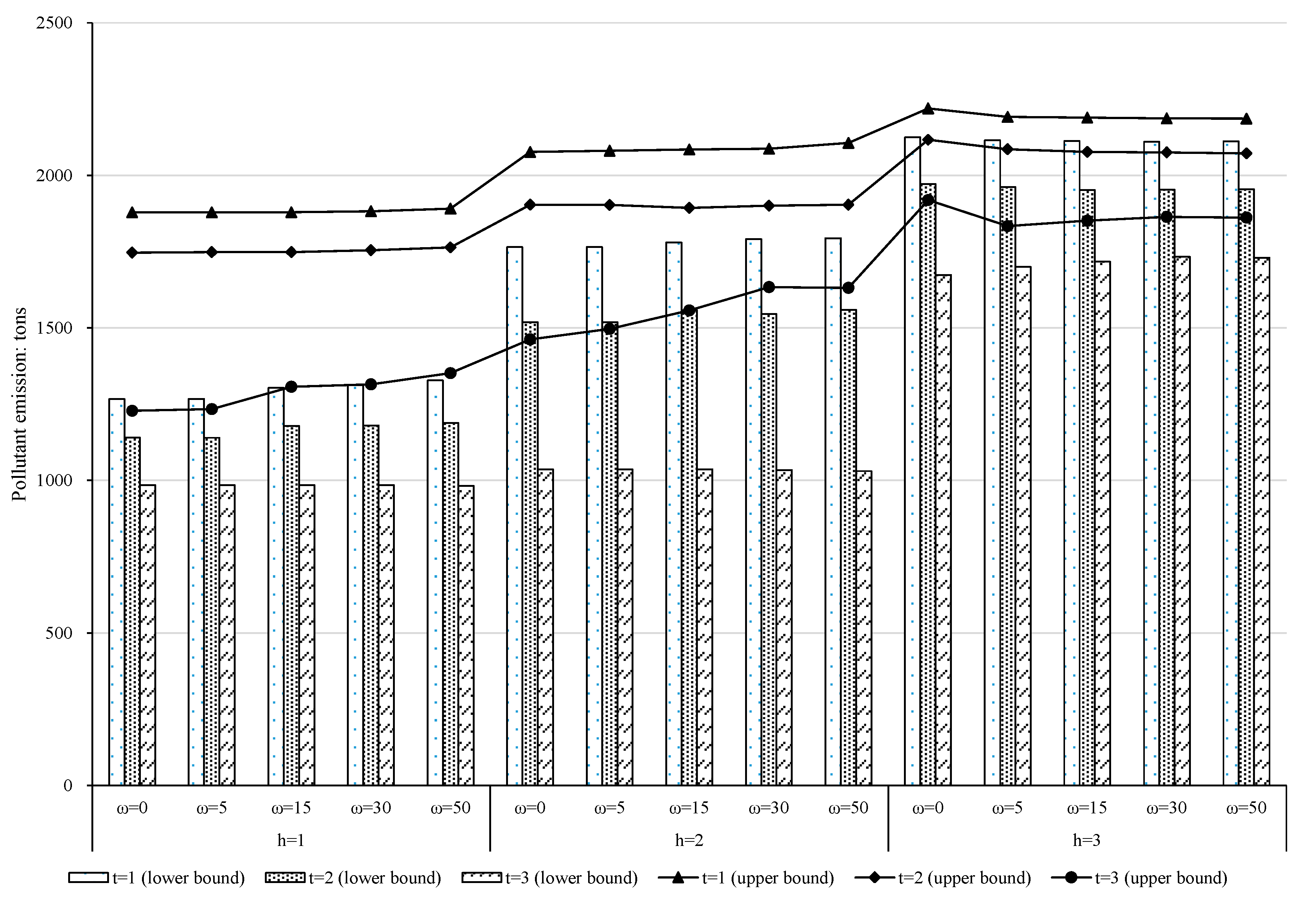
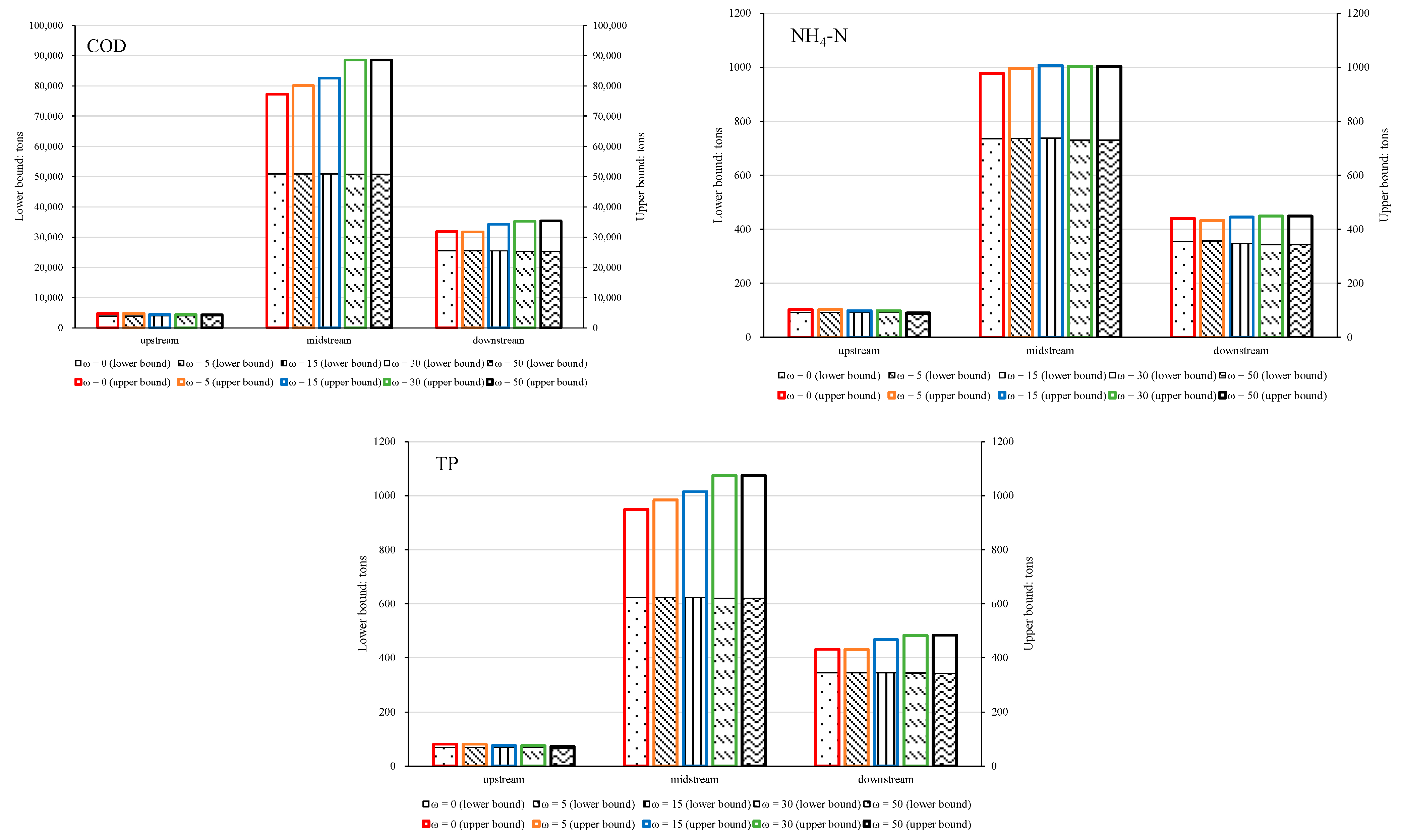
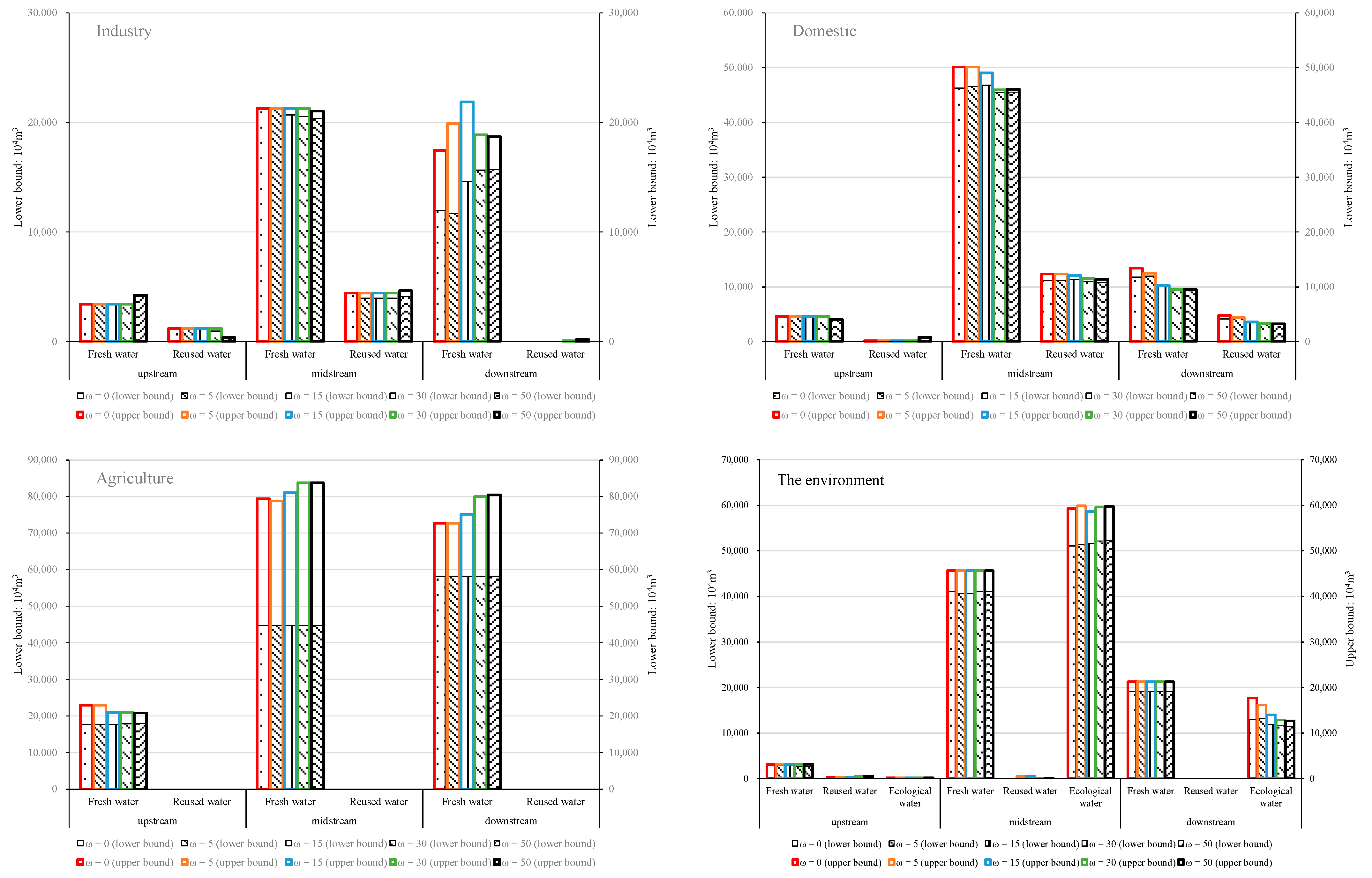
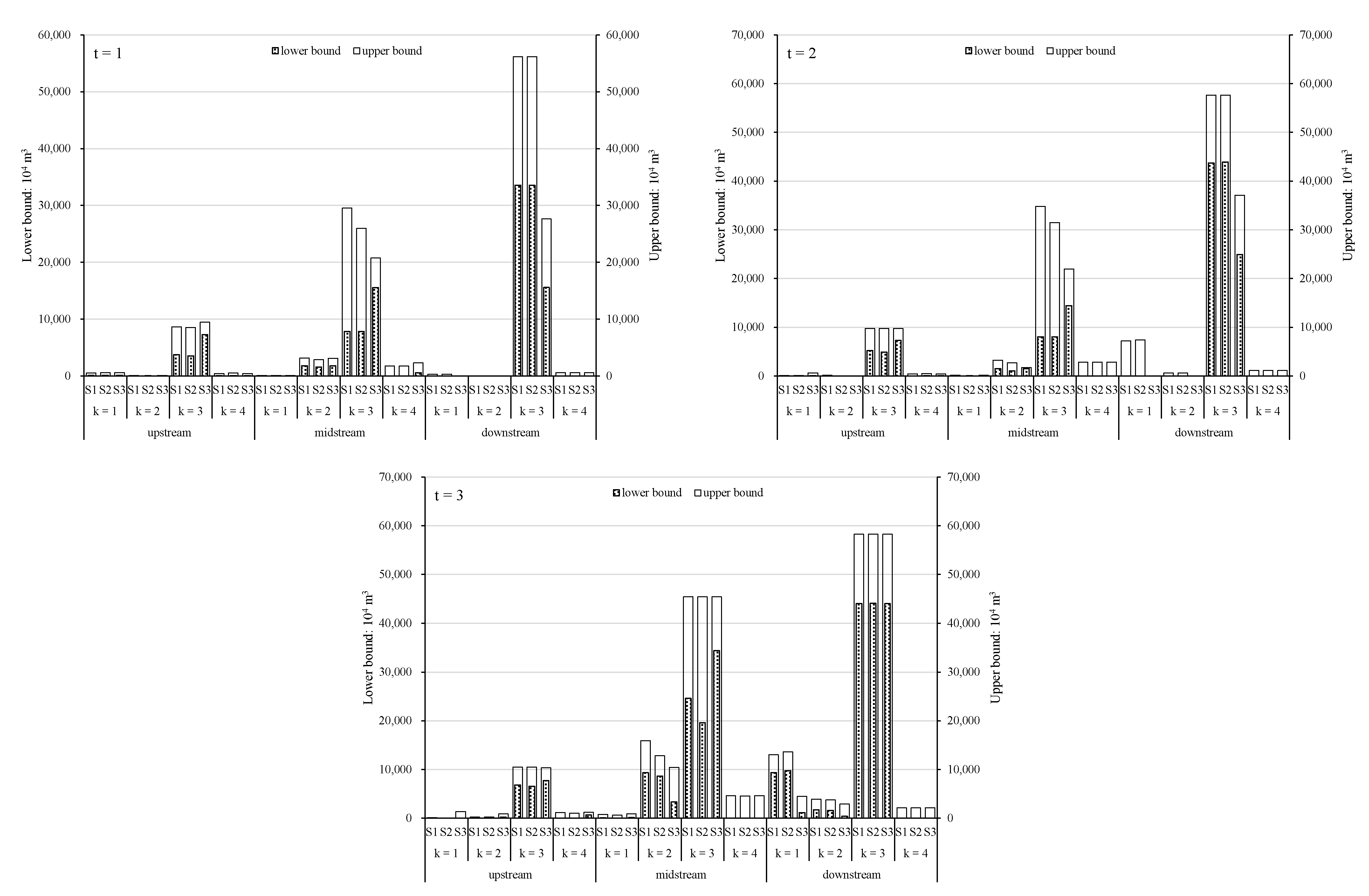
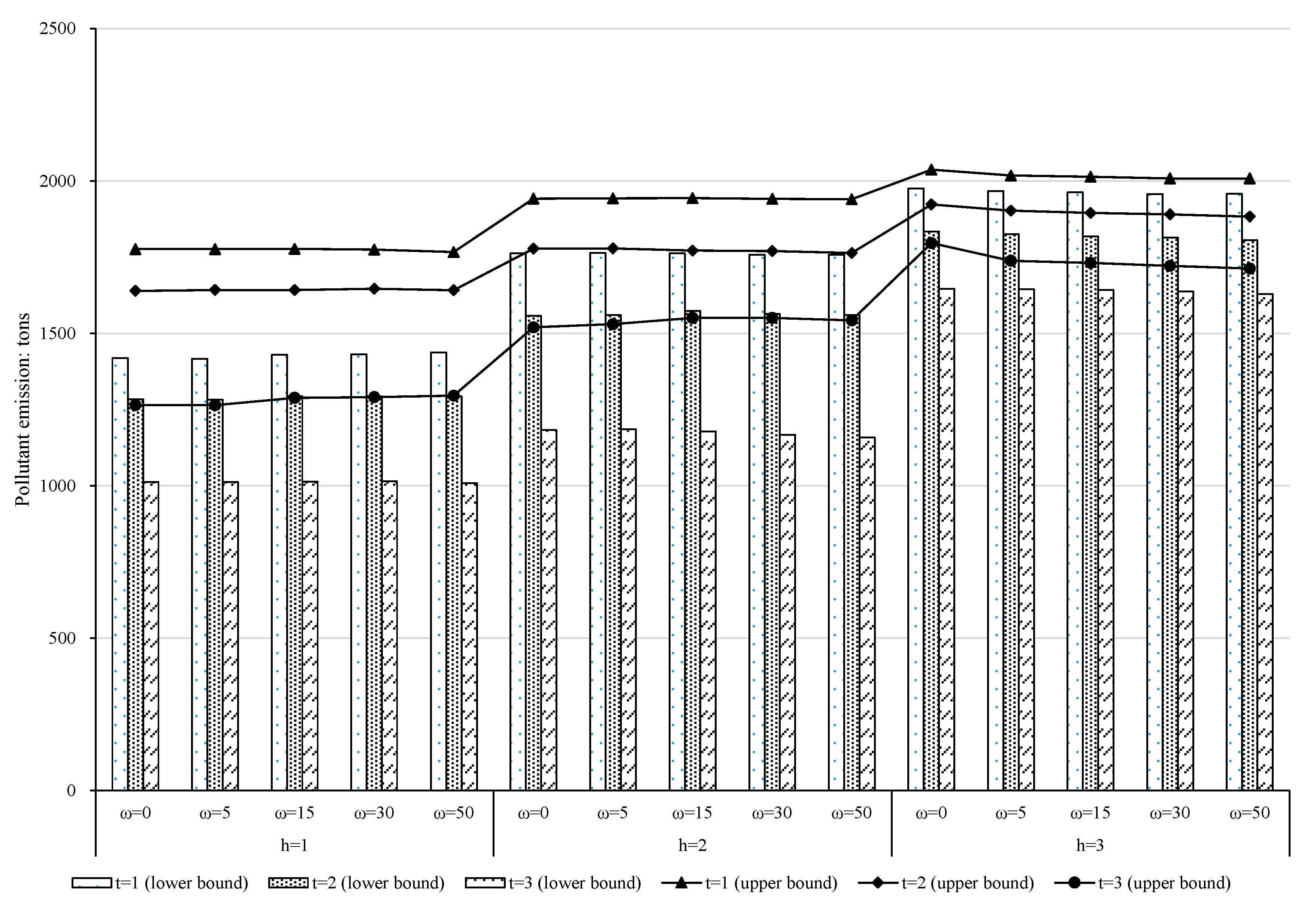
3.2. Water Resource Allocation and Pollutant Emissions

In this section, we comprehensively analyzed the pollutant emissions and water resource allocation strategies of the Fenhe River Basin under different risk control levels, to study the key constraints of the sustainable development of the basin. Figure 5, Figure 6, and Figure 7 show the emissions of the main pollutants (COD, NH₄-H, and TP) during the study periods. These figures indicate that emissions of the three pollutants gradually increase for scenarios 1, 2, and 3, which are influenced by the increasing water resources and environmental carrying capacities. For example, in period 1, for ω values of 15, the amounts of TP emission Figure 7 are [1303.04, 1879.12], [1779.22, 2084.21], and [2112.36, 2188.52] tons for scenarios 1, 2, and 3, respectively. In periods 2 and 3, the amounts are [1178.63, 1748.45], [1556.89, 1893.39], and [1952.14, 2076.31] tons and [984.26, 1306.73], [1035.78, 1557.28], and [1717.21, 1850.83] tons. These show a downward trend of pollutant emissions over time due to the requirement of water quality improvement. As ω values increase, the stronger risk control constraint leads to the optimization of water resource allocation strategies, and the pollutant emissions show different tendencies. For period 3 and scenario 2, the amounts of COD emissions Figure 5 are [80,355.82, 114,004.60], [80,400.54, 116,705.51], [80,383.72, 121,337.26], [80,177.29, 128,239.97], and [80,097.39, 128,220.25] tons, showing an obvious upward trend for $\omega$ values increasing from 0 to 30, and the same as NH₄-H and TP. For period 2 and the same scenario, emissions of the three pollutants show slight and different fluctuations. The amounts of COD emissions fluctuate with [118,727.20, 150,165.3], [118,685.06, 150,216.61], and [121,704.1, 149,513.43] tons for $\omega$ values of 0, 5, and 15, and gradually increase to [120,761.79, 149,996.61] and [121,912.25, 150,347.08] tons for $\omega$ values of 30 and 50. For NH₄-H, the amounts are [1558.24, 1778.04], [1560.31, 1778.67], [1572.82, 1771.39], [1563.26, 1769.81], and [1559.74, 1763.8] tons, showing a downward trend for $\omega$ values of 5, 15, 30, and 50. Unlike the COD and NH₄-H, the amounts of TP emissions are [1519.19, 1903.4], [1518.64, 1902.73], [1556.89, 1893.39], [1545.2, 1900.39], and [1558.55, 1903.6] tons, showing an upward trend for $\omega$ values of 5, 15, 30, and 50. These differences are closely related to regional industrial structures, water resource allocation strategies for sectors, and various pollutant emission intensities. Additionally, Figure 5, Figure 6 and Figure 7 show more significant changes in period 3, and datasets such as the available water resources for scenario 2 are closer to regional policies and plans; thus, the following analysis would be carried out for period 3, scenario 2.

Figure 8 shows regional differences of pollutant emissions. The upstream area has the smallest pollutant emissions and shows a gradual downward trend as $\omega$ values increase. For example, the amounts of COD emissions are [3937.51, 4802.34], [3937.51, 4802.34], [3974.81, 4426.28], [4030.00, 4426.28], and [3961.33, 4320.60] tons for $\omega$ values of 0, 5, 15, 30, and 50, respectively, the same as for NH₄-H and TP, which indicates that in the upstream area, sectors with lower benefits also have relatively low pollutant emission intensities. In the other areas, pollutant emissions show different tendencies. In the downstream area, COD, NH₄-H, and TP emissions generally increase as $\omega$ values increase, with a slight decrease in $\omega$ values of 5. For example, the amounts of NH₄-H are [355.05, 440.1], [356.01, 431.55], [348.29, 444.86], [342.95, 448.68], [342.74, 448.99] tons for values of 0, 5, 15, 30 and 50, respectively. However, in the midstream, unlike COD and TP emissions that show an upward trend as $\omega$ values increase, the amounts of NH₄-H emissions are [735.3, 977.58], [736.81, 996.49], [737.97, 1007.52], [731.11, 1004.21], and [730.86, 1003.87] tons, which fluctuate and show a downward trend for $\omega$ values of 15, 30, and 50. The changes in pollutant emissions reflect the optimization of water resource allocation strategies and the differences in factors such as the industrial structure, water benefit, and environmental carrying capacity in different areas of the basin.

Figure 9 shows the water resource allocation for different sectors. In the upstream area, the total industry and domestic water consumption remains unchanged as $\omega$ values increase, while the amounts of allocated fresh water and reused water for the two sectors have changed for $\omega$ values of 50. The water consumption of agriculture shows a downward trend, and the amounts are [17,643.79, 23,006.55], [17,643.79, 23,006.55], [17,643.79, 20,985.81], [17,870.91, 20,985.81], and [17,893.23, 20,839.33] × 10⁴ m³. Considering the downward trend of sectoral risks and pollutant emissions, the decrease in total water consumption demonstrates that benefits and costs are the main factors affecting resource allocation strategies for agriculture in the upstream area. In the midstream area, water resource allocations show differences across the four sectors. Water consumption of the industry remains unchanged as $\omega$ values increase due to relatively high sectoral benefits. Water consumption of the domestic and agriculture sectors shows opposite tendencies. Fresh water and reuse water for the domestic sector are [46,283.31, 50,081.57], [46,578.61, 50,081.57], [46,784.56, 49,036.18], [45,442.33, 45,956.5], and [45,534.13, 46,025.65] × 10⁴ m³ and [11,221.41, 12,351.39], [11,226.32, 12,351.39], [11,296.26, 12,040.38], [10,971.21, 11,503.76], and [10,769.79, 11,360.53] × 10⁴ m³ for $\omega$ values of 0, 5, 15, 30, and 50, and these show a gradual downward trend. Oppositely, as $\omega$ values increase, more water resources are allocated to agriculture in order to balance sectoral benefits. The same tendency appears in the downstream area for the two sectors. However, water resource allocation strategies for the industry show obvious fluctuation; the amounts of fresh water are [11,962.2, 17,436.72], [11,682.12, 19,914.18], [14,637.63, 21,864.76], [15,646.56, 18,878.45], and [15,688.91, 18,691.18] × 10⁴ m³ for $\omega$ values of 0, 5, 15, 30, and 50. Considering the downward trend of industrial risks in this area, it indicates that the developed ITSDP model optimizes water resource allocations based on different regional industrial structures and benefits.

Additionally, ecological water consumption in this study reflects the gaps between pollutant emissions and environmental carrying capacity for different values, showing various changes due to regional and sectoral differences in pollutant emission intensities. In the midstream area, it shows fluctuation, and the amounts of ecological water are [51,044.31, 59,268.6], [51,313.11, 59,856.65], [51,626.08, 58,622.38], [52,122.75, 59,570.23], and [52,225.92, 59,707.16] × 10⁴ m³. In the upstream and downstream areas, the amounts of ecological water show a downward trend as values increase; the developed model optimizes water resource allocation and reduces pollutant quantities entering the river in these areas.

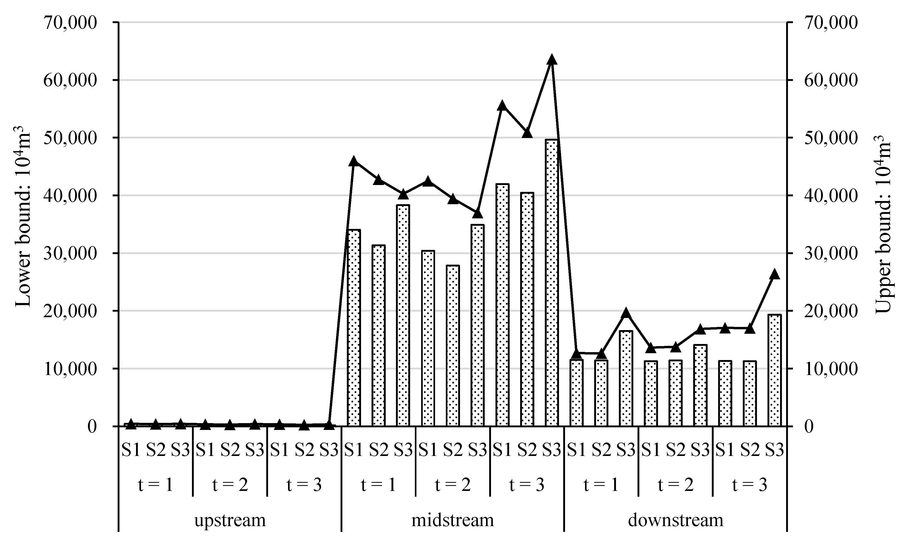
3.3. Policy Scenarios Analysis

Risks and ecological water consumption indicate that water resources are insufficient for coordinating watershed socio-economic development and ensuring environmental quality in the Fenhe River basin. In this section, we set up two policy intervention scenarios to study the potential effect of appropriate policy interventions for further optimization of water resource allocation. To reflect the severe water shortage conditions, we consider a low water resource level (h = 1) and a $\omega$ value of 15 as the baseline scenario (S1), and another two policy scenarios are set: (1) S2: The water reuse rate gradually increases 10% over time; (2) S3: Coordinating the transferred water resources in the whole river basin for optimal regulation.

The risks in the three scenarios (

Table 4. Benefits of water resource utilization and risks in the Fenhe River Basin (CNY 10⁶ million).

	Periods	Policy Scenarios
		S1	S2	S3
Benefits	t = 1	[5.89, 6.68]	[5.91, 6.69]	[5.94, 6.69]
	t = 2	[8.23, 10.46]	[8.25, 10.51]	[8.61, 10.46]
	t = 3	[10.22, 14.67]	[10.36, 14.77]	[11.97, 15.39]
Risks	t = 1	[0.09, 0.18]	[0.08, 0.16]	[0.08, 0.13]
	t = 2	[0.08, 0.39]	[0.05, 0.37]	[0.06, 0.16]
	t = 3	[0.54, 2.07]	[0.51, 1.94]	[0.11, 0.33]

) are CNY [0.09, 0.18], [0.08, 0.16], and [0.08, 0.13] × 10⁶ million in period 1, CNY [0.08, 0.39], [0.05, 0.37], and [0.06, 0.16]× 10⁶ million, and CNY [10.22, 14.67], [10.36, 14.77], and [11.97, 15.39] × 10⁶ million in periods 2 and 3. The results indicate that improving the water reuse rate (S2) and coordinating the water resources of the whole river basin (S3) could increase the benefits and control regional risks, and S3 shows a more significant effect. The results can support decision makers to formulate water management requirements and coordinate the optimal allocation of water resources in the entire river basin.

Figure 10 shows the deficits in water resource pre-allocations in different scenarios. The results show a regional difference. For example, in period 1, the water deficits of agriculture in S2 decrease from [3753.41, 8668.13] × 10⁴ m³ (S1) to [3539.54, 8535.12] × 10⁴ m³, and in S3, they increase to [7255.75, 9467.58] × 10⁴ m³. In the midstream and downstream areas, the results show different changes. The agricultural scale in the upstream area is relatively below, and S3 regulates the transferred water resources in the whole river basin, which leads to more water resources being allocated to other areas of higher benefits.

Figure 11 shows ecological water supplies in different scenarios. Compared to the other scenarios, S2 has fewer ecological water supplies; for example, the amounts are [34,046.38, 46,012.89] × 10⁴ m³ (S1), [31,367.80, 42,790.44] × 10⁴ m³, and [38,340.87, 40,257.44] × 10⁴ m³ (S3). A higher water reuse rate means fewer pollutant emissions. Additionally, the amounts of ecological water under S3 are the largest in the midstream area in period 2, compared to the downstream area. For example, the amounts of ecological water are [41,982.57, 55,669.92] × 10⁴ m³ (S1), [40,475.93, 50,915.65] × 10⁴ m³ (S2), and [49,665.20, 63,614.76] × 10⁴ m³ (S3), respectively. It indicates that more water resources are allocated to the production sectors with higher benefits over the river basin. Water shortages mainly appear in the downstream areas, according to requirements of water resources and environment protection. The results show that water recycling is a critical factor for addressing water shortage and reducing pollutant emissions, and appropriate policy interventions would further optimize water resource allocation and effectively alleviate water shortage and water pollution in the Fenhe River Basin.

4. Conclusions

In this study, an improved ITSDP model was built for optimal water resource allocation and pollutant emissions under dual constraints and uncertainties in the Fenhe River Basin, a highly urbanized, densely populated, typically water-deprived area with high degrees of contamination. The proposed model simultaneously addresses the uncertainties presented as interval values and probability distributions by integrating the IPP and TSP methods. The introduction of the downside risk aversion method effectively avoids possible risks caused by uneven water resource allocations. By solving the ITSDP model, optimal water resource allocation and pollutant emissions for the primary water use sectors were calculated for the programming periods under different scenarios. Additionally, we obtained the amounts of ecological water supplies required for purifying excessive pollutant emissions to identify areas with significant environmental water problems. These results, such as pollutant emissions and ecological water supplies, subject to strong water quality constraints, could provide a basis for regional emission permit systems. Furthermore, the optimal results under different risk levels and policy scenarios, namely S2 and S3, could reflect the subjective will of decision-makers for regional socio-economic development, environment protection, and possible changes of regional planning and policies.

The aim of this study was to use the ITSDP model to develop an effective approach to determine and optimize water resource allocations. The coordination of water quality protection and socio-economic development could support the establishment of water-based industrial structures and layouts. The results suggest that this approach is applicable and effective for the optimization of water resource allocation and water quality management in the Fenhe River Basin and could also be applied in other contexts or water-stressed areas. However, this model does not consider the gross ecosystem production from water resources utilizations, which has been a significant indicator of regional sustainable development. Further studies are needed to address these limitations.

References

1. Edda, K.; Thomas, K.; Olaf, K.; Elisabeth, K.; Jörg, S.; Gunda, R.; Georg, T.; Dietrich, B.; Peter, K. Integrated Water Resources Management under different hydrological, climatic and socio-economic conditions. Environ. Earth Sci. 2012, 65, 1363–1366. [Google Scholar]
2. Ran, L.; Lu, X.X. Redressing China’s strategy of water resource exploitation. Environ. Manag. 2013, 51, 503–510. [Google Scholar] [CrossRef] [PubMed]
3. Liang, X.D.; Zhang, R.Y.; Liu, C.M.; Liu, H.Y. Quantitative Measurement of the Sustainable Water Resource Development System in China Inspired by Dissipative Structure Theory. Sustainability 2018, 10, 3996. [Google Scholar] [CrossRef] [Green Version]
4. Liu, L.; Ma, J.; Hao, X.; Li, Q. Limitations of Water Resources to Crop Water Requirement in the Irrigation Districts along the Lower Reach of the Yellow River in China. Sustainability 2019, 11, 4680. [Google Scholar] [CrossRef] [Green Version]
5. Zhang, H.; Lu, P.; Zhang, D.; Kou, S.; Mao, Y. Watershed-scale assessment of surface water-related risks from shale gas development in mountainous areas, China. J. Environ. Manag. 2020, 279, 111589. [Google Scholar] [CrossRef]
6. Kavan, Š.; Kročová, Š.; Pokorný, J. Assessment of the Readiness and Resilience of Czech Society against Water-Related Crises. Hydrology 2021, 8, 14. [Google Scholar] [CrossRef]
7. Xu, J.P.; Lv, C.L.; Yao, L.M.; Hou, S.H. Intergenerational equity based optimal water allocation for sustainable development: A case study on the upper reaches of Minjiang River, China. J. Hydrol. 2019, 568, 835–848. [Google Scholar] [CrossRef]
8. Wei, F.; Zhang, X.; Xu, J.; Bing, J.; Pan, G. Simulation of water resource allocation for sustainable urban development: An integrated optimization approach. J. Clean. Prod. 2020, 273, 122537. [Google Scholar] [CrossRef]
9. Fu, M.R.; Guo, B.; Wang, W.J.; Wang, J.; Zhao, L.H.; Wang, J.L. Comprehensive Assessment of Water Footprints and Water Scarcity Pressure for Main Crops in Shandong Province, China. Sustainability 2019, 11, 1–18. [Google Scholar] [CrossRef] [Green Version]
10. Long, K.S.; Pijanowski, B.C. Is there a relationship between water scarcity and water use efficiency in China? A national decadal assessment across spatial scales. Land Use Policy 2017, 69, 502–511. [Google Scholar] [CrossRef]
11. Tian, J.; Guo, S.; Liu, D.; Pan, Z.; Hong, X. A Fair Approach for Multi-Objective Water Resources Allocation. Water Resour. Manag. 2019, 33, 3633–3653. [Google Scholar] [CrossRef]
12. Qin, J.; Fu, X.; Peng, S.; Huang, S. An Integrated Decision Support Framework for Incorporating Fairness and Stability Concerns into River Water Allocation. Water Resour. Manag. 2020, 34, 211–230. [Google Scholar] [CrossRef]
13. Read, L.; Madani, K.; Inanloo, B. Optimality versus stability in water resource allocation. J. Environ. Manag. 2014, 133, 343–354. [Google Scholar] [CrossRef] [PubMed]
14. Wang, Z.Q.; Yang, J.; Deng, X.Z.; Lan, X. Optimal Water Resources Allocation under the Constraint of Land Use in the Heihe River Basin of China. Sustainability 2015, 7, 1558–1575. [Google Scholar] [CrossRef] [Green Version]
15. Wang, J.F.; Cheng, G.D.; Gao, Y.G.; Long, A.H.; Xu, Z.M.; Xin, L.; Chen, H.; Barker, T. Optimal Water Resource Allocation in Arid and Semi-Arid Areas. Water Resour. Manag. 2008, 22, 239–258. [Google Scholar] [CrossRef]
16. Kročová, Š.; Kavan, Š. Cooperation in the Czech Republic border area on water management sustainability. Land Use Policy 2019, 86, 351–356. [Google Scholar] [CrossRef]
17. Choi, I.-C.; Shin, H.-J.; Nguyen, T.T.; Tenhunen, J. Water Policy Reforms in South Korea: A Historical Review and Ongoing Challenges for Sustainable Water Governance and Management. Water 2017, 9, 717. [Google Scholar] [CrossRef] [Green Version]
18. Hobbs, B.F. Bayesian Methods for Analysing Climate Change and Water Resource Uncertainties. J. Environ. Manag. 1997, 49, 53–72. [Google Scholar] [CrossRef] [Green Version]
19. Wilby, R.L. Uncertainty in water resource model parameters used for climate change impact assessment. Hydrol. Process. 2010, 19, 3201–3219. [Google Scholar] [CrossRef]
20. Hart, O.E.; Halden, R.U. On the need to integrate uncertainty into U.S. water resource planning. Sci. Total Environ. 2019, 691, 1262–1270. [Google Scholar] [CrossRef] [PubMed]
21. Yao, L.; Xu, Z.; Chen, X. Sustainable Water Allocation Strategies under Various Climate Scenarios: A Case Study in China. J. Hydrol. 2019, 574, 529–543. [Google Scholar] [CrossRef]
22. Karmakar, S.; Mujumdar, P.P. An inexact optimization approach for river water-quality management. J. Environ. Manag. 2006, 81, 233–248. [Google Scholar] [CrossRef]
23. Li, Y.P.; Huang, G.H.; Nie, S.L. An interval-parameters multi-stage stochastic programming model for water resources management under uncertainty. Adv. Water. Resour. 2006, 29, 776–789. [Google Scholar] [CrossRef]
24. Qin, X.; Huang, G.; Chen, B.; Zhang, B. An interval-parameter waste-load-allocation model for river water quality management under uncertainty. Environ. Manag. 2009, 43, 999. [Google Scholar] [CrossRef] [PubMed]
25. Xie, Y.L.; Li, Y.P.; Huang, G.H.; Li, Y.F.; Chen, L.R. An inexact chance-constrained programming model for water quality management in Binhai New Area of Tianjin, China. Sci. Total Environ. 2011, 409, 1757–1773. [Google Scholar] [CrossRef] [PubMed]
26. Li, J.; Qiao, Y.; Lei, X.; Kang, A.; Wang, M.; Liao, W.; Wang, H.; Ma, Y. A two-stage water allocation strategy for developing regional economic-environment sustainability. J. Environ. Manag. 2019, 244, 189–198. [Google Scholar] [CrossRef]
27. Huang, G.H.; Loucks, D.P. An inexact two stage stochastic programming model for water resources management under uncertainty. Civ. Eng. Environ. Syst. 2000, 17, 95–118. [Google Scholar] [CrossRef]
28. Maqsood, I.; Huang, G.H.; Huang, Y.F.; Chen, B. ITOM: An interval parameter two-stage optimization model for stochastic planning of water resources systems. Stoch. Environ. Res. Risk Assess. 2005, 19, 125–133. [Google Scholar] [CrossRef]
29. Xu, Y.; Huang, G.H.; Qin, X.S. Inexact two-stage stochastic robust optimization model for water resources management under uncertainty. Environ. Eng. Sci. 2009, 26, 1765–1776. [Google Scholar] [CrossRef]
30. Li, W.; Li, Y.P.; Li, C.H.; Huang, G.H. An inexact two-stage water management model for planning agricultural irrigation under uncertainty. Agric. Water Manag. 2010, 97, 1905–1914. [Google Scholar] [CrossRef]
31. Wang, S.; Huang, G.H. Interactive two-stage stochastic fuzzy programming for water resources management. J. Environ. Manag. 2011, 92, 1986–1995. [Google Scholar] [CrossRef]
32. Xie, Y.L.; Huang, G.H.; Li, W.; Li, J.B.; Li, Y.F. An inexact two-stage stochastic programming model for water resources management in Nansihu Lake Basin, China. J. Environ. Manag. 2013, 127, 188–205. [Google Scholar] [CrossRef] [PubMed]
33. Sarband, E.M.; Araghinejad, S.; Attari, J. Developing an Interactive Spatial Multi-Attribute Decision Support System for Assessing Water Resources Allocation Scenarios. Water Resour. Manag. 2020, 34, 447–462. [Google Scholar] [CrossRef]
34. Xie, Y.L.; Huang, G.H. Development of an inexact two-stage stochastic model with downside risk control for water quality management and decision analysis under uncertainty. Stoch. Environ. Res. Risk Assess. 2014, 28, 1555–1575. [Google Scholar] [CrossRef]
35. Harlow, W.V. Asset Allocation in a Downside-Risk Framework. Financ. Anal. J. 1991, 47, 28–40. [Google Scholar] [CrossRef]
36. Park, J.; Park, S.; Yun, C.; Kim, Y. Integrated model for financial risk management in refinery planning. Ind. Eng. Chem. Res. 2009, 49, 129. [Google Scholar] [CrossRef]
37. Finger, R. Expanding risk consideration in integrated models-the role of downside risk aversion in irrigation decisions. Environ. Model. Softw. 2013, 43, 169–172. [Google Scholar] [CrossRef]
38. Lee, S.Y.; Lee, I.B.; Han, J. Design under uncertainty of carbon capture, utilization and storage infrastructure considering profit, environmental impact, and risk preference. Appl. Energy 2019, 238, 34–44. [Google Scholar] [CrossRef]
39. Xiao, J.; Wang, L.Q.; Deng, L.; Jin, Z.D. Characteristics, sources, water quality and health risk assessment of trace elements in river water and well water in the Chinese Loess Plateau. Sci. Total Environ. 2018, 650, 2004–2012. [Google Scholar] [CrossRef]
40. Yang, G.D.; Meng, Q.Z.; Sun, L.H. Present situation of water environment and sustainable development countermeasures for economy and environment in Fenhe River Valley. China Popul. Resour. Environ. 2001, S1, 65–67. [Google Scholar]
41. Kang, N. Analysis on the Spatiotemporal Features of Precipitation during 1971–2011 in the Fenhe River Basin. Master’s Thesis, Shanxi University, Taiyuan, China, 2015. [Google Scholar]
42. Yang, Y.G.; Qin, Z.D.; Xue, Z.J. Study on Hydrology and Water Resources in the Fen River Basin; Science Press: Beijing, China, 2016; pp. 53–55. [Google Scholar]
Figure 1. Framework for the inexact downside risk aversion and two-stage programming model.
Sustainability 13 10835 g001
Figure 2. Geographical position and study area of the Fenhe River Basin.
Sustainability 13 10835 g002
Figure 3. Benefits and risks in the Fenhe River Basin at different risk levels.
Sustainability 13 10835 g003
Figure 4. Sectoral risks in the Fenhe River Basin at different risk levels.
Sustainability 13 10835 g004
Figure 5. COD emissions in the Fenhe River Basin at different risk levels.
Sustainability 13 10835 g005
Figure 6. NH4-H emissions in the Fenhe River Basin at different risk levels.
Sustainability 13 10835 g006
Figure 7. TP emissions in the Fenhe River Basin at different risk levels.
Sustainability 13 10835 g007
Figure 8. Pollutant emissions in the Fenhe River Basin in period 3, scenario 2.
Sustainability 13 10835 g008
Figure 9. Water resource allocation strategies for sectors in the Fenhe River Basin.
Sustainability 13 10835 g009
Figure 10. Water resource deficits in the Fenhe River Basin.
Sustainability 13 10835 g010
Figure 11. Ecological water supplies in the Fenhe River Basin in different scenarios.
Sustainability 13 10835 g011