
Analytical Models for CO2 Emissions and Travel Time for Short-to-Medium-Haul Flights Considering Available Seats


Abstract
:1. Introduction
2. Background
2.1. Environmental Impact of Aviation and Mitigation Strategies
2.1.1. Technological Improvements
2.1.2. Emissions’ Compensation
2.1.3. Modal Substitution
2.2. Computation of Aviation Emissions
3.Methodology and Model Development
- Estimation of emissions and travel time for individual aircraft types:
- −
- First, a historical analysis of which aircraft types are used on different routes was performed so that their operational range (maximum distance usage) could be established;
- −
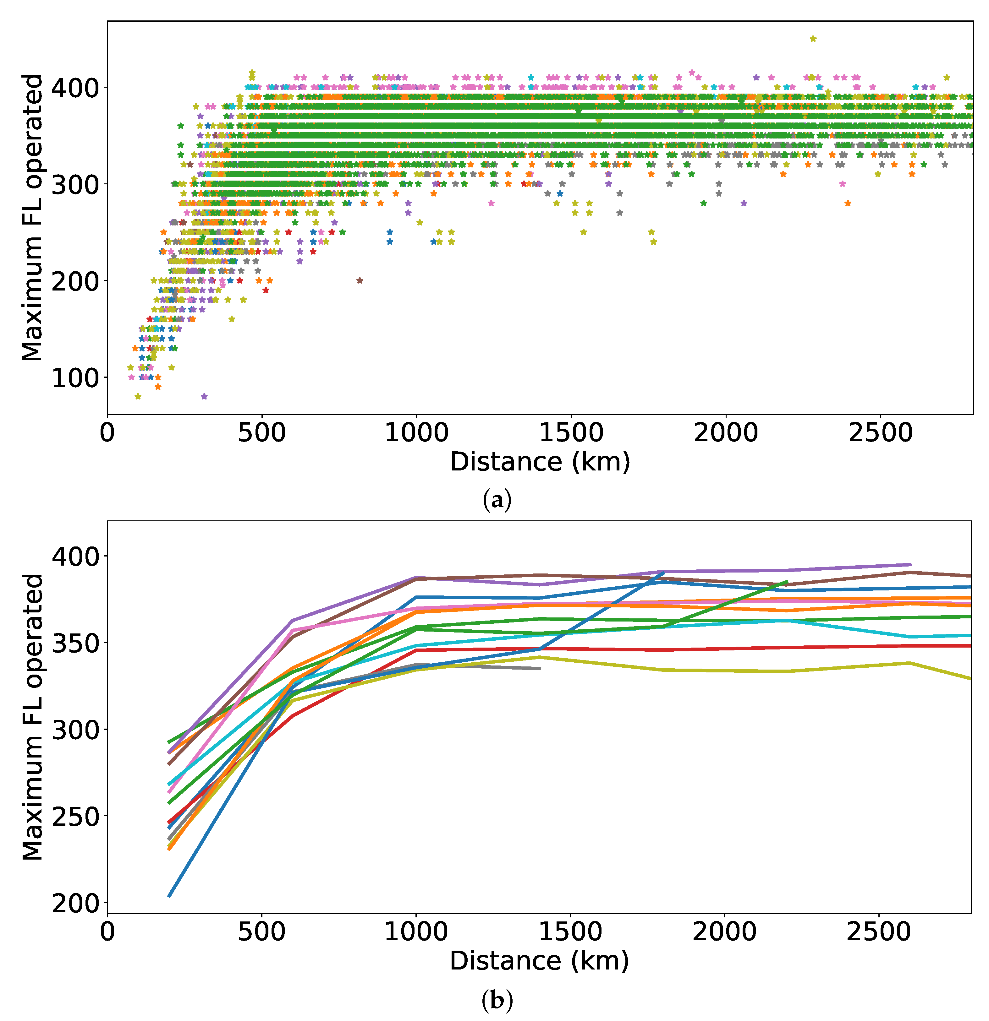
- Then, an analysis of which flight levels were selected as a function of the distance to be covered was performed;
- −
- An analysis was also carried out to identify the seats available per aircraft type;
- −
- EUROCONTROL’s IMPACT model was used to estimate emissions per aircraft type every 50km in their domain of use considering the FL previously identified. In this case, nominal weights, speed and vertical profiles were used;
- −
- Time and fuel corrections were applied afterwards to account for inefficiencies in the system, e.g., distance flown between the origin and destination longer than GCD, and ground operations (taxi-in and taxi-out) to obtain the estimate of gate-to-gate time and emissions per individual flight;
- The definition of generic analytical models depending on GCD between the origin and destination and on the number of available seats provided, computed as the fittings of the individual flights’ performances previously computed.
3.1. Historical Traffic Analysis
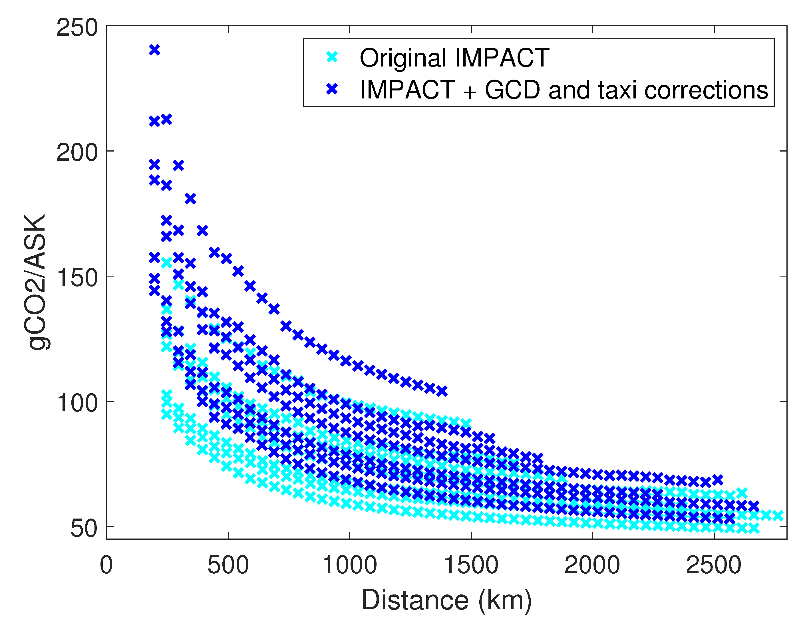
3.2. IMPACT Fuel and Time Computations
3.3. Correction Factors
3.3.1. Distance Correction
3.3.2. Fuel and Time Taxi Corrections
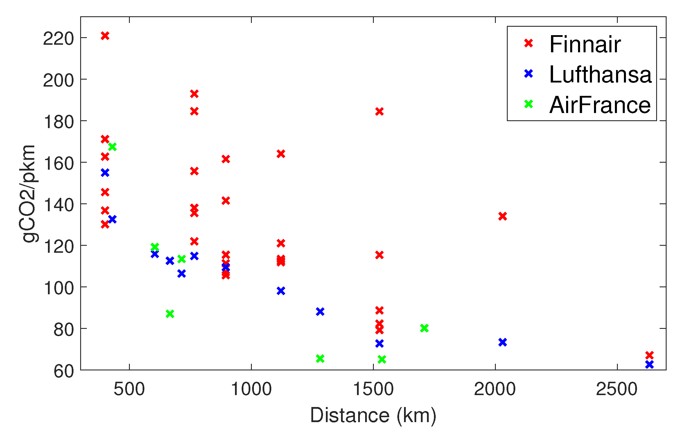
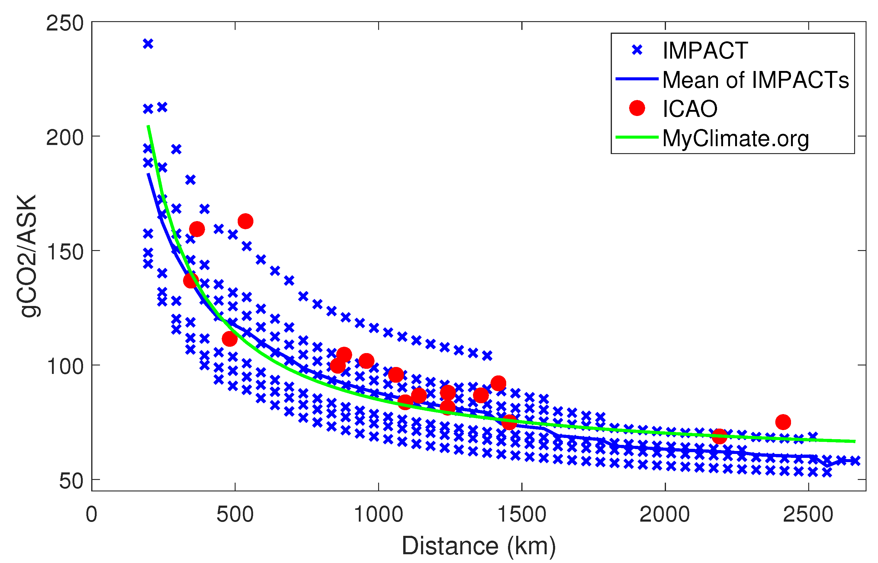
3.4. Comparison of Individual Emission Estimations with Other Calculators
3.5. Analytical Model Development
3.5.1. CO and Gate-to-Gate Time Estimations
3.5.2. Analytical Fitting
CO Emissions
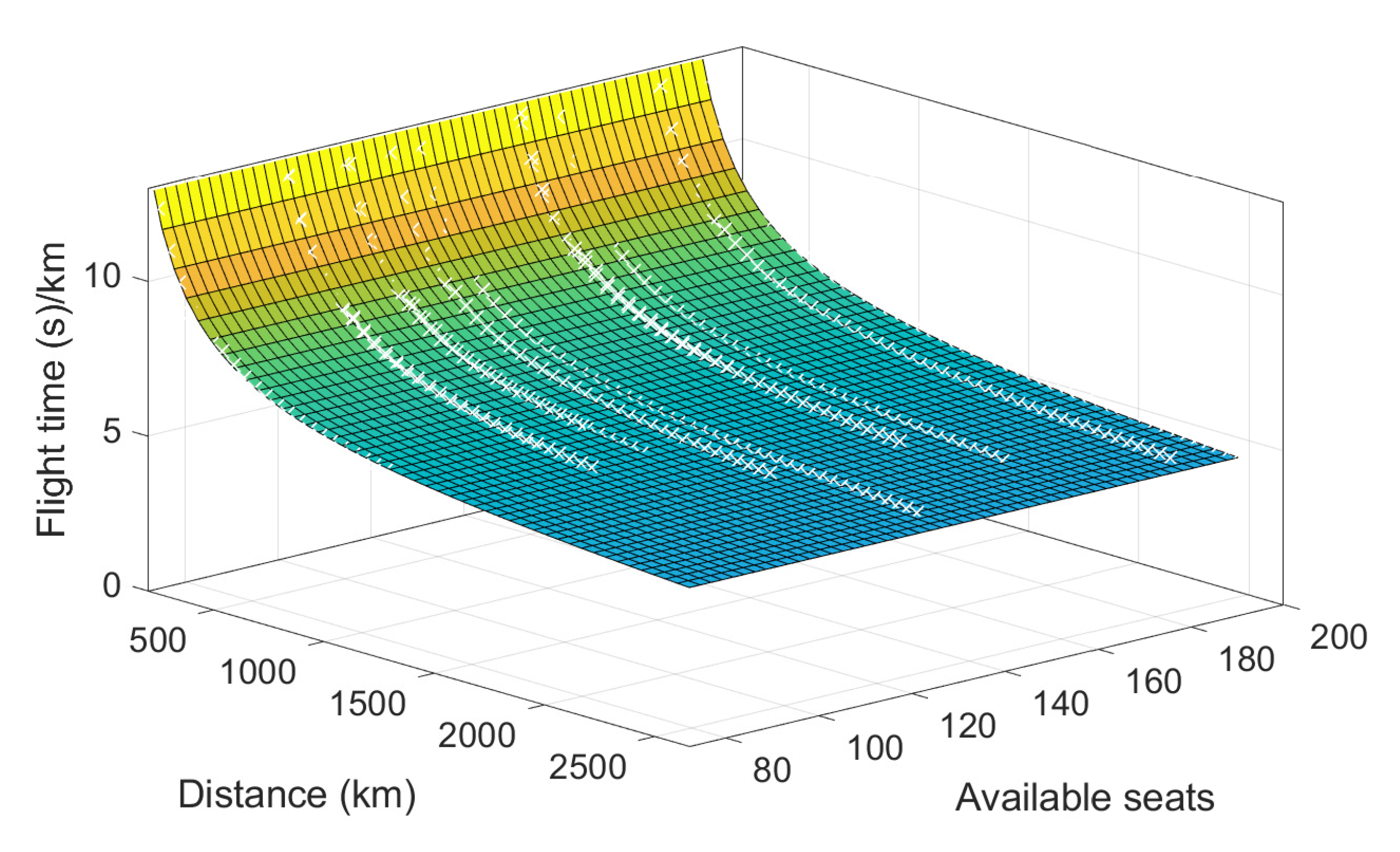
Gate-to-Gate Time
3.5.3. Accuracy of the Analytical Fitting
4. Application
4.1. Analysis of Emissions in the Short-Haul Western European Network
4.1.1. Methodology
4.1.2. Results
4.2. Comparison with Rail
4.2.1. Methodology
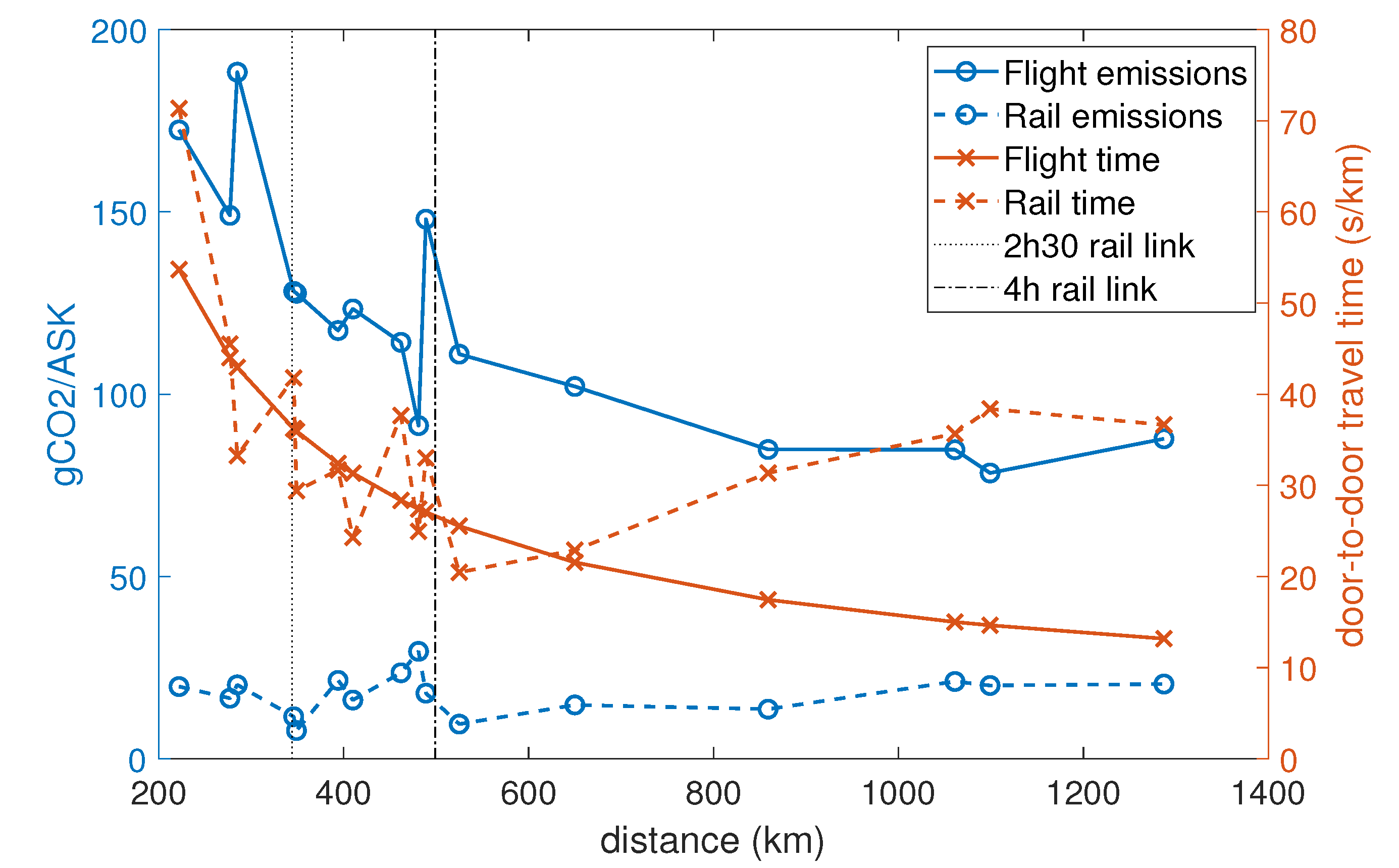
4.2.2. Results
5. Discussion
Author Contributions
Funding
Institutional Review Board Statement
Informed Consent Statement
Data Availability Statement
Acknowledgments
Conflicts of Interest
References
- EUROCONTROL. Challenges of Growth—European Aviation in 2040. 2018. Available online: www.eurocontrol.int/publication/challenges-growth-2018 (accessed on 14 September 2021).
- EUROCONTROL. Performance Review Report An Assessment of Air Traffic Management in Europe during the Calendar Year 2019. 2020. Available online: www.eurocontrol.int/sites/default/files/2020-06/eurocontrol-prr-2019.pdf (accessed on 14 September 2021).
- SESAR Joint Undertaking. European ATM Master Plan—Executive View. 2020. Available online: www.sesarju.eu/masterplan2020 (accessed on 14 September 2021).
- Clean Sky 2. Joint Technical Programme. 2015. Available online: ec.europa.eu/research/participants/data/ref/h2020/other/guide-appl/jti/h2020-guide-techprog-cleansky-juen.pdf (accessed on 14 September 2021).
- DLR. DEPA 2050—Development Pathways for Aviation up to 2050. Technical Report, German Aerospace Center. 2020. Available online: http://elib.dlr.de/142185/1/DEPA2050_StudyReport.pdf (accessed on 14 September 2021).
- European Commission. Regulation (EU) 2017/2392 of the European Parliament and of the Council of 13 December 2017 Amending Directive 2003/87/EC to Continue Current Limitations of Scope for Aviation Activities and to Prepare to Implement a Global Market-Based Measure from 2021. 2017. Available online: www.legislation.gov.uk/eur/2017/2392/adopted/data.pdf (accessed on 14 September 2021).
- ICAO. Resolution A40-19: Consolidated Statement of Continuing ICAO Policies and Practices Related to Environmental Protection—Carbon Offsetting and Reduction Scheme for International Aviation (CORSIA). 2019. Available online: www.icao.int/environmental-protection/Documents/Assembly/ResolutionA40-19CORSIA.pdf (accessed on 14 September 2021).
- Convention Citoyenne pour le Climat. Avis de la Convention Citoyenne Pour le Climat sur les Réspones Apportées par le Gouvernement à ses Propositions. 2021. Available online: www.conventioncitoyennepourleclimat.fr/wp-content/uploads/2021/03/CCC-rapportSession8GR-1.pdf (accessed on 14 September 2021).
- Lederer, P.; Nambimadom, R. Airline network design. Oper. Res. 1998, 46, 785–804. [Google Scholar] [CrossRef]
- Trapote-Barreira, C. Methodology for Optimal Design of Efficient air Transport Networks in a Competitive Environment. Ph.D. Thesis, Universitat Politecnica de Catalunya, Barcelona, Spain, 2015. [Google Scholar]
- Grimme, W.; Maertens, S.; Bingemer, S.; Gelhausen, M. Estimating the market potential for long-haul narrowbody aircraft using origin-destination demand and flight schedules data. Transp. Res. Procedia 2021, 52, 412–419. Available online: www.sciencedirect.com/science/article/pii/S2352146521000892 (accessed on 14 September 2021). [CrossRef]
- Cooper, T.; Reagan, I.; Porter, C.; Franzoni, C. Global Fleet and MRO Market Forecast 2021–2031. Technical Report, Oliver Wyman. 2021. Available online: www.oliverwyman.com/content/dam/oliver-wyman/v2/media/2021/feb/GlobalFLeetandMROMarketForecast2021-2031OW.pdf (accessed on 14 September 2021).
- IATA. IATA Carbon Offset Program—Frequently Asked Questions. Version 10.1. 2020. Available online: https://www.iata.org/contentassets/922ebc4cbcd24c4d9fd55933e7070947/icop_faq_general-for-airline-participants.pdf (accessed on 14 September 2021).
- EEA. EEA Greenhouse Gas—Data Viewer. Available online: www.eea.europa.eu/data-and-maps/data/data-viewers/greenhouse-gases-viewer (accessed on 14 April 2021).
- Lee, D.; Fahey, D.; Forster, P.; Newton, P.; Wit, R.; Lim, L.; Sausen, R. Aviation and global climate change in the 21st century. Atmos. Environ. 2009, 43, 3520–3537. [Google Scholar] [CrossRef] [Green Version]
- Lee, D.; Fahey, D.; Skowron, A.; Allen, M.; Burkhardt, U.; Chen, Q.; Doherty, S.; Freeman, S.; Forster, P.; Fuglestvedt, J.; et al. The contribution of global aviation to anthropogenic climate forcing for 2000 to 2018. Atmos. Environ. 2021, 244, 117834. [Google Scholar] [CrossRef]
- IATA. Aircraft Technology Roadmap to 2050. 2020. Available online: www.iata.org/contentassets/8d19e716636a47c184e7221c77563c93/technology20roadmap20to20205020no20foreword.pdf (accessed on 14 September 2021).
- Jiménez-Crisóstomo, A.; Rubio-Andrada, L.; Celemín-Pedroche, M. The Constrained Air Transport Energy Paradigm in 2021. Sustainability 2021, 13, 2830. [Google Scholar] [CrossRef]
- Prussi, M.; Konti, A.; Lonza, L. Could Biomass Derived Fuels Bridge the Emissions Gap between High Speed Rail and Aviation? Sustainability 2019, 11, 1025. [Google Scholar] [CrossRef] [Green Version]
- Anderson, K. The inconvenient truth of carbon offsets. Nature 2012, 484, 7. [Google Scholar] [CrossRef]
- Polonsky, M.J.; Grau, S.L.; Garma, R. The New Greenwash?: Potential Marketing Problems with Carbon Offsets. Int. J. Bus. Stud. 2010, 18, 49–54. [Google Scholar]
- Arnaldo Valdés, R.; Gomez Comendador, V.; Braga Campos, L. How Much Can Carbon Taxes Contribute to Aviation Decarbonization by 2050. Sustainability 2021, 13, 1086. [Google Scholar] [CrossRef]
- Markham, F.; Young, M.; Reis, A.; Higham, J. Does carbon pricing reduce air travel? Evidence from the Australian ‘Clean Energy Future’ policy, July 2012 to June 2014. J. Transp. Geogr. 2018, 70, 206–214. [Google Scholar] [CrossRef] [Green Version]
- Ministère de la Transition Ecologique. Projet de loi Climat & Résilience—Les Députés Viennent de finir L’examen des Articles du Titre III « Se déplacer » : Ça Change Quoi Dans nos Vies? Available online: www.ecologie.gouv.fr/projet-loi-climat-resilience-deputes-viennent-finir-lexamen-des-articles-du-titre-iii-se-deplacer-ca (accessed on 3 June 2021).
- Baumeister, S. Replacing short-haul flights with land-based transportation modes to reduce greenhouse gas emissions: The case of Finland. J. Clean. Prod. 2019, 225, 262–269. [Google Scholar] [CrossRef]
- Baumeister, S.; Leung, A. The emissions reduction potential of substituting short-haul flights with non-high-speed rail (NHSR): The case of Finland. Case Stud. Transp. Policy 2021, 9, 40–50. [Google Scholar] [CrossRef]
- Robertson, S. The potential mitigation of CO2 emissions via modal substitution of high-speed rail for short-haul air travel from a life cycle perspective—An Australian case study. Transp. Res. Part D Transp. Environ. 2016, 46, 365–380. [Google Scholar] [CrossRef]
- Spinetta, J. L’avenir du Transport Ferroviaire. Rapport au Premier Ministre. 2018. Available online: www.ecologie.gouv.fr/sites/default/files/2018.02.15Rapport-Avenir-du-transport-ferroviaire.pdf (accessed on 14 September 2021).
- EEA. EMEP/EEA air Pollutant Emission Inventory Guidebook 2019, 1.A.3.a Aviation 1 Master Emissions Calculator 2019. 2019. Available online: www.eea.europa.eu/publications/emep-eea-guidebook-2019/part-b-sectoral-guidance-chapters/1-energy/1-a-combustion/1-a-3-a-aviation-1-annex5-LTO/view (accessed on 14 September 2021).
- EEA. EMEP/EEA Air Pollutant Emission Inventory Guidebook 2019, 1.A.3.a Aviation 2019. 2019. Available online: www.eea.europa.eu/publications/emep-eea-guidebook-2019/part-b-sectoral-guidance-chapters/1-energy/1-a-combustion/1-a-3-a-aviation/view (accessed on 14 September 2021).
- ICAO. Carbon Emissions Calculator. Available online: www.icao.int/environmental-protection/CarbonOffset/Pages/default.aspx (accessed on 14 May 2021).
- ICAO. Carbon Emissions Calculator Methodology. Version 11. 2018. Available online: www.icao.int/environmental-protection/CarbonOffset/Documents/Methodology%20ICAO%20Carbon%20Calculatorv11-2018.pdf (accessed on 14 September 2021).
- Foundation Myclimate. Offset Your Flight Emissions! Available online: http://co2.myclimate.org/en/flight_calculators/new. (accessed on 14 May 2021).
- Foundation Myclimate. The myclimate Flight Emission Calculator. 2019. Available online: www.myclimate.org/fileadmin/userupload/myclimate-home/01Information/01Aboutmyclimate/09Calculationprinciples/Documents/myclimate-flight-calculator-documentationEN.pdf (accessed on 14 September 2021).
- Schäfer, A.; Evans, A.; Reynolds, T.; Dray, L. Costs of Mitigating CO2 Emissions from Passenger Aircraft. Nat. Clim. Chang. 2016, 6, 412–417. Available online: https://www.nature.com/articles/nclimate2865 (accessed on 14 September 2021). [CrossRef] [Green Version]
- Dray, L. AIM2015: Documentation, 2019. Air Transportation Systems Lab. UCL Energy Institute. Available online: http://www.atslab.org/wp-content/uploads/2019/12/AIM-2015-Documentation-v9-122019.pdf (accessed on 14 September 2021).
- Lissys. Piano-X: Aircraft Emissions and Performance. User’s Guide. 2008. Available online: https://www.lissys.uk/piano-x-guide.pdf (accessed on 14 September 2021).
- Swan, W.; Adler, N. Aircraft trip cost parameters: A function of stage length and seat capacity. Transp. Res. Part E Logist. Transp. Rev. 2006, 42, 105–115. [Google Scholar] [CrossRef]
- De Lemos, F.; Woodward, J. Calculating block time and consumed fuel for an aircraft model. Aeronaut. J. 2021, 125, 847–878. [Google Scholar] [CrossRef]
- Baumeister, S. ‘Each Flight is Different’: Carbon emissions of selected flights in three geographical markets. Transp. Res. Part D: Transp. Environ. 2017, 57, 1–9. [Google Scholar] [CrossRef] [Green Version]
- Park, Y.; O’Kelly, M. Fuel burn rates of commercial passenger aircraft: Variations by seat configuration and stage distance. J. Transp. Geogr. 2014, 41, 137–147. [Google Scholar] [CrossRef]
- European Union Aviation Safety Agency (EASA). ICAO Aircraft Engine Emissions Databank. Available online: https://www.easa.europa.eu/domains/environment/icao-aircraft-engine-emissions-databank (accessed on 14 September 2021).
- AIRFRANCE. Calculateur Carbone. Available online: http://corporate.airfrance.com/fr/co2/calculateur (accessed on 27 May 2021).
- FINNAIR. Finnair Emissions Calculator. Available online: www.finnair.com/FI/GB/emissions-calculator (accessed on 27 May 2021).
- COMPENSAID Lufthansa. Compensate Your Flight. Available online: http://lufthansa.compensaid.com/contribute/flights (accessed on 27 May 2021).
- Delgado, L.; Prats, X. En Route Speed Reduction Concept for Absorbing Air Traffic Flow Management Delays. J. Aircr. 2012, 49, 214–224. [Google Scholar] [CrossRef]
- Delgado, L.; Prats, X. Effect of Wind on Operating-Cost-Based Cruise Speed Reduction for Delay Absorption. IEEE Trans. Intell. Transp. Syst. 2013, 14, 918–927. [Google Scholar] [CrossRef]
- EUROCONTROL. RECAT-EU—European Wake Turbulence Categorisation and Separation Minima on Approach and Departure. Edition: 1.2. Edition Date: 14 February 2018. Available online: www.eurocontrol.int/sites/default/files/2021-07/recat-eu-released-september-2018.pdf (accessed on 30 August 2021).
- SeatGuru. Find Your Seat Map. Available online: www.seatguru.com (accessed on 2 June 2021).
- EUROCONTROL. Integrated Aircraft Noise and Emissions Modelling Platform. Available online: www.eurocontrol.int/platform/integrated-aircraft-noise-and-emissions-modelling-platform (accessed on 14 April 2021).
- EUROCONTROL. Taxi Times—Winter 2019–2020. Available online: www.eurocontrol.int/publication/taxi-times-winter-2019-2020 (accessed on 14 May 2021).
- Khadilkar, H.; Balakrishnan, H. Estimation of Aircraft Taxi-out Fuel Burn using Flight Data Recorder Archives. In Proceedings of the AIAA Guidance, Navigation, and Control Conference, Portland, OR, USA, 8–11 August 2011. [Google Scholar]
- EUROCONTROL. Aviation Intelligence Unit. Flying the ‘Perfect Green Flight’: How Can We Make Every Journey as Environmentally Friendly as Possible? 2021. Think Paper #10. Available online: https://www.eurocontrol.int/publication/eurocontrol-think-paper-10-flying-perfect-green-flight (accessed on 14 September 2021).
- European Rail Timetable. European Rail Timetable. May 2021. Available online: http://www.europeanrailtimetable.eu (accessed on 14 September 2021).
- EcoPassenger. Compare the Energy Consumption, the CO2 Emissions and other Environmental Impacts for Planes, Cars and Trains in Passenger Transport. Available online: http://ecopassenger.hafas.de/bin/query.exe/en?L=vs_uic& (accessed on 2 June 2021).
- Knörr, W.; Hüttermann, R. EcoPassenger Environmental Methodology and Data Update. Institut für Energie- und Umweltforschung Heidelberg gGmbH. 2016. Available online: http://ecopassenger.hafas.de/hafas-res/download/Ecopassenger_Methodology_Data.pdf (accessed on 14 September 2021).
- Eurostat. Energy Statistics—Quantities, Annual Data. 2015. Available online: http://ec.europa.eu/eurostat/data/database (accessed on 14 September 2021).
- International Energy Agency. Key World Energy Statistics; IEA: Paris, France, 2015. [Google Scholar] [CrossRef]
- DLR. Airport Accessibility in Europe (Edition 1.02). Technical Report, Air Transport and Airport Research. 2010. Available online: http://ec.europa.eu/transport/sites/default/files/modes/air/studies/doc/intermodality/2010-airport-accessibility-in-eu.pdf (accessed on 14 September 2021).
- Transportation Research Board. TCRP Report 165: Transport Capacity and Quality of Service Manual. Third Edition. 2013. Available online: www.trb.org/Main/Blurbs/169437.aspx (accessed on 14 September 2021).
- Babikian, R.; Lukachko, S.P.; Waitz, I.A. The historical fuel efficiency characteristics of regional aircraft from technological, operational, and cost perspectives. J. Air Transp. Manag. 2002, 8, 389–400. [Google Scholar] [CrossRef] [Green Version]
- Ryerson, M.S.; Hansen, M. The potential of turboprops for reducing aviation fuel consumption. Transp. Res. Part D Transp. Environ. 2010, 15, 305–314. [Google Scholar] [CrossRef]


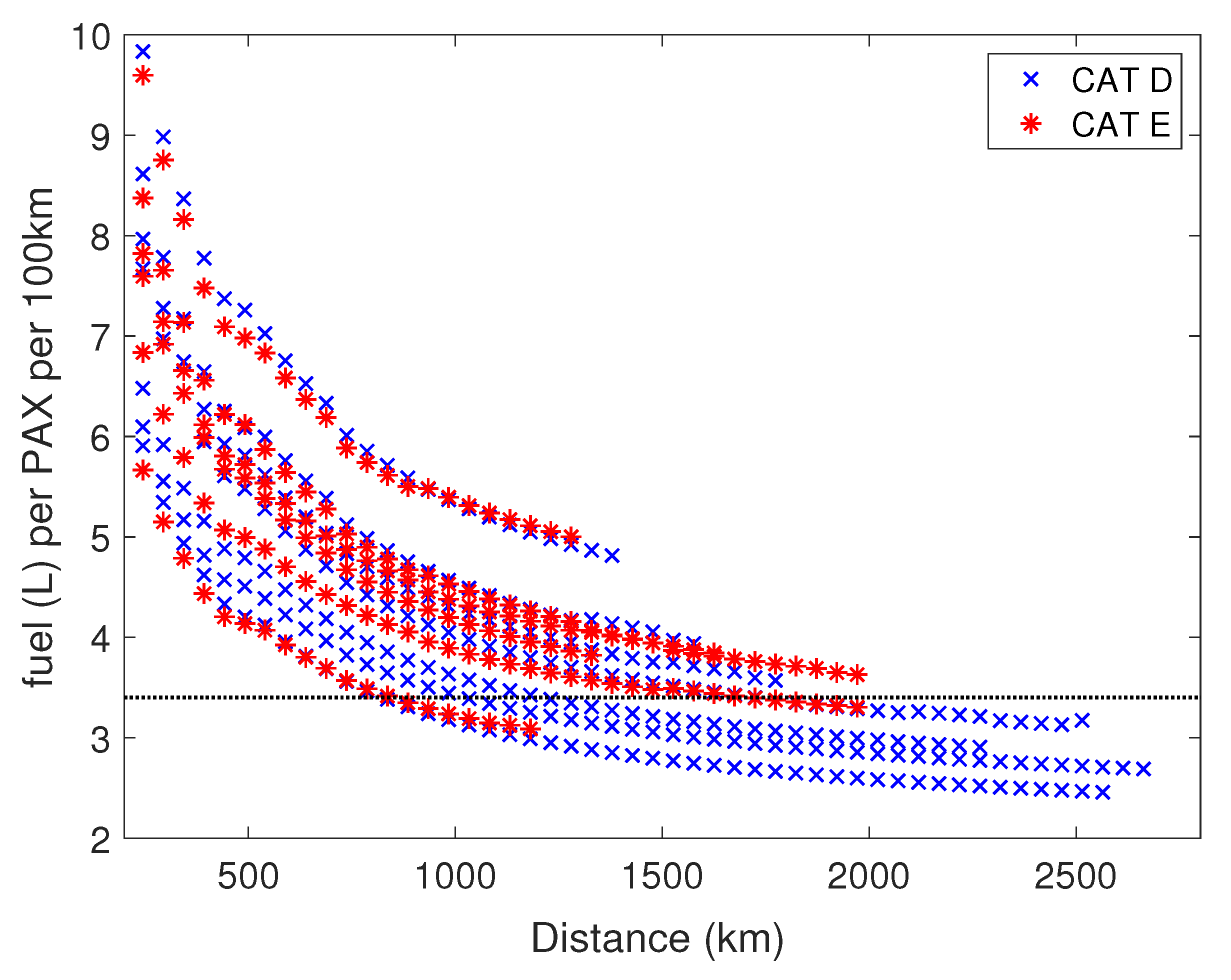
| RECAT-EU Category | Aircraft Types |
|---|---|
| CAT E | CRJX, E195, E190, B734, B735, B712 |
| CAT D | A321, A320, A319, A318, B738, B737, B736 |
| Model | SSE | R-Square | RMSE |
|---|---|---|---|
| CO (g) emissions per seat per kilometre | g | g | |
| Time (s) per kilometre | s | s |
| DEP | ARR | d (km) | IMP gCO/pkm | FIT gCO/pkm | Error % | |
|---|---|---|---|---|---|---|
| LFPG | LFLL | 406.15 | 128 | 125.11 | 129.74 | 3.70 |
| LEBL | LEMD | 476.87 | 128 | 116.16 | 121.15 | 4.30 |
| LEBL | LEMD | 476.87 | 190 | 89.99 | 86.12 | 4.29 |
| LEBL | LFPG | 845.43 | 128 | 92.32 | 97.70 | 5.83 |
| LEBL | LFPG | 845.43 | 158 | 77.00 | 83.39 | 8.30 |
| LEBL | LFPG | 845.43 | 190 | 72.56 | 68.13 | 6.10 |
| LEMD | LFPG | 158 | 72.11 | 77.83 | 7.93 | |
| LFPG | UUEE | 158 | 60.02 | 61.95 | 3.22 | |
| LFPG | UUEE | 190 | 56.80 | 58.78 | 3.48 |
| DEP | ARR | GCD (km) | Time (h) | kgCO/PAX |
|---|---|---|---|---|
| Faro | Lisboa | 222 | 3.57 | 4.40 |
| Porto | Lisboa | 277 | 2.67 | 4.60 |
| Madrid | Valencia | 285 | 1.80 | 5.78 |
| London | Paris | 346 | 3.18 | 4.00 |
| London | Brussels | 349 | 2.02 | 2.70 |
| Madrid | Sevilla | 394 | 2.63 | 8.48 |
| Paris | Lyon | 410 | 1.93 | 6.61 |
| Berlin | Munich | 462 | 4.00 | 10.90 |
| Barcelona | Madrid | 481 | 2.50 | 10.80 |
| Paris | Stuttgart | 489 | 3.65 | 8.80 |
| Paris | Bordeaux | 525 | 2.15 | 5.00 |
| Paris | Marseille | 650 | 3.30 | 7.30 |
| Paris | Barcelona | 859 | 6.65 | 11.70 |
| Paris | Madrid | 1061 | 10.52 | 22.50 |
| Paris | Roma | 1099 | 11.72 | 22.10 |
| Paris | Napoli | 1287 | 13.10 | 26.40 |
Publisher’s Note: MDPI stays neutral with regard to jurisdictional claims in published maps and institutional affiliations. |
© 2021 by the authors. Licensee MDPI, Basel, Switzerland. This article is an open access article distributed under the terms and conditions of the Creative Commons Attribution (CC BY) license (https://creativecommons.org/licenses/by/4.0/).
Share and Cite
Montlaur, A.; Delgado, L.; Trapote-Barreira, C. Analytical Models for CO2 Emissions and Travel Time for Short-to-Medium-Haul Flights Considering Available Seats. Sustainability 2021, 13, 10401. https://doi.org/10.3390/su131810401
Montlaur A, Delgado L, Trapote-Barreira C. Analytical Models for CO2 Emissions and Travel Time for Short-to-Medium-Haul Flights Considering Available Seats. Sustainability. 2021; 13(18):10401. https://doi.org/10.3390/su131810401
Chicago/Turabian StyleMontlaur, Adeline, Luis Delgado, and César Trapote-Barreira. 2021. "Analytical Models for CO2 Emissions and Travel Time for Short-to-Medium-Haul Flights Considering Available Seats" Sustainability 13, no. 18: 10401. https://doi.org/10.3390/su131810401
APA StyleMontlaur, A., Delgado, L., & Trapote-Barreira, C. (2021). Analytical Models for CO2 Emissions and Travel Time for Short-to-Medium-Haul Flights Considering Available Seats. Sustainability, 13(18), 10401. https://doi.org/10.3390/su131810401