Meteorological and Hydrological Drought Analysis and Its Impact on Water Quality and Stream Integrity

Abstract

Rising temperature and shifting precipitation patterns due to climate change are likely to intensify droughts throughout the world. Understanding the drought characteristics of possible future scenarios under climate change requires verification of past drought events using appropriate drought indices. Consequently, this study investigates the application of two widely used drought indices, the standardized precipitation index (SPI) and standardized streamflow index (SSI), to characterize historical droughts, drought trends, and their impact on water quality and stream integrity for a selected study basin in New Jersey. Results indicated that both SPI and SSI were able to identify historical drought events, including three drought emergency periods and the most recent drought-watch periods. A significant positive meteorological drought was observed at the western side of the basin, whilst a significant positive hydrological drought was found in the eastern side. The average pollutant concentration of drought periods were lesser than non-drought periods due to reduction of different processes, such as erosion and transport of sediment and nutrients into rivers and streams, during drought periods as opposed to non-drought periods. The findings from this study will serve to bolster the ongoing efforts to formulate better drought management strategies for future climate change in the Raritan Basin.

1. Introduction

Drought is a complex and recurring phenomenon that has detrimental impacts on agriculture, economy, water supply, and ecosystems [1,2]. Out of all environmental disasters, drought is considered to be the least understood despite tremendous progress in the hydrological sciences [3,4,5]. The definition of drought changes from one study to another depending on the objective of the study and the types of water usage that are of concern. For example, a certain level of decrease in a river’s water level may not be crucial for the aquatic ecosystems’ health, whilst the same level of decrease could cause severe consequences in a small reservoir for water supply purposes. Unlike other natural hazards such as floods, the onset and cessation of drought are not clearly defined, making it more challenging to characterize. Furthermore, the advent of global climate change is likely to further aggravate the drought evolution concomitant with severe consequences due to accelerated hydrological processes in the landscape [6,7]. The increase in global temperature has altered the spatiotemporal pattern of drought events [8]. Using satellite-based, combined moisture-thermal condition index, Kogan et al. [9] pointed out that the world drought area increased approximately 2 to 5% for all intensities, including severe to exceptional, extreme to exceptional, and exceptional categories, during 1998 to 2014 due to intensification of global warming. McCabe and Wolock [10] observed that roughly 2% of global land area were in drought throughout all the years since 1901 to 2009 by using month-by-month potential evapotranspiration and long-term mean monthly precipitation data. These study results depicted a statistically significant positive drought trend at a 95% confidence level. Additionally, Song et al. [11] demonstrated that the secure trend of meteorological drought index changed from −0.001 in 1950 to −0.383 during 2014, indicating an increasing global drought trend.

Drought is defined as a shortage of water in the form of either precipitation, streamflow, or soil moisture as compared to normal conditions in a given hydrological system [4,12]. Droughts are primarily classified into four categories, including meteorological, hydrological, agricultural, and socioeconomic [13,14,15]. The severity and duration of droughts does not remain constant in a whole watershed with respect to time and location. Therefore, spatio-temporal analysis of aforementioned droughts are prerequisite for formulation of better water resources planning and management within a basin.

Drought indices are used as proxies to describe drought characteristics; however, the performance of drought indices in tracking and quantifying drought events may vary from one location to another due to inherent complexity of the drought phenomenon in conjunction with availability of good, quality data. Therefore, identifying and formulating accurate drought indices plays a paramount role in formulating successful mitigation strategies for a drought-prone basin. A number of drought indices have been developed and used to characterize drought processes, its propagation in different components of the hydrological cycle, and impacts around the globe. Some of the most commonly used drought indices are standardized precipitation index (SPI) [16,17,18], Palmer drought severity index (PDSI) [19,20,21], standardized precipitation and evapotranspiration index (SPEI) [6,22], rainfall deciles (RD) [23], standardized streamflow index (SSI) [24,25], Palmer hydrological drought index (PHDI) [19], surface water supply index (SWSI) [26,27], Palmer moisture anomaly index (PMAI) [19,20,21], and computed soil moisture (CSM) [28,29,30]. Out of all drought indices, SPI and SSI are selected for drought analysis in this study, as both drought indices can be calculated for variety of accumulation periods (i.e. 1 month, 3 months, 6 months, and 12 months), which facilitates investigation of the impacts of drought not only from agricultural production point of view but also from water supply prospective in the region. Agricultural production is related to availability of soil moisture, which is the reflection of precipitation anomalies in the shorter accumulation period, such as one month. Additionally, water supply to urban areas depends on water availability in the streams and rivers, which is the reflection of longer accumulation precipitation anomalies, including 6 months and 12 months. Therefore, use of these drought indices will help us to formulate better water resources management policies from both agricultural production as well as water supply prospective in the study area.

Several studies have used SPI and SSI to assess drought characteristics, including frequency, duration, magnitude, and severity, in different parts of the world. For example, Byakatonda et al. [6] used SPI in conjunction with Mann–Kendall test and Sen’s slope estimator to characterize drought severity for different accumulation periods in the Botswana region located in southern Africa. They observed that SPI was able to identify historical drought events as well as a positive wetting trend depicting an increase in precipitation in the study area. Using SPI and SSI as drought indices, Barker et al. [31] highlighted spatial variability of meteorological drought in the United Kingdom (U.K.), whilst a more severe hydrological drought was noticed in the south and east side of the U.K. Marini et al. [3] investigated spatio-temporal drought characteristics in the Apulia region in southern Italy using SPI. Results indicated an increasing drought severity trend in the western part of the region but a decreasing trend in the eastern part. Bacanli [32] conducted a drought study in the Aegean region of Turkey using SPI of 1-to 12-months accumulation period. Results suggested more frequent drought for shorter accumulation periods (i.e., three months), whilst an increase in accumulation periods increased drought duration with decreased drought frequency. Wu et al. [33] used SPI for a shorter accumulation period for selected weather station in the contiguous United States. They revealed that SPI values for shorter accumulation periods can reasonably explain droughts monitored in the eastern United States, while the interpretation of SPI index is complicated in the western United States due to presence of distinct seasonal precipitation effect. Modarres [24] conducted a streamflow drought study in western Isfahan province, Iran, using SSI index. He found that seasonal autoregressive integrated moving average model concomitant with SSI index was reasonable in forecasting drought severity. Vicente-Serrano et al. [34] used SSI index combined with two different approaches (best monthly fit and minimum orthogonal distance) to compute accurate streamflow drought in the Erbo Basin in Spain.

It is evident that these drought indices have been used throughout the globe to facilitate better water resources planning and management. However, indices developed in one location cannot be extrapolated to others. Consequently, it is important to investigate the degree to which drought indices can accurately explain drought characteristics at different spatio-temporal scales across a basin. This study proposes to employ SPI and SSI to investigate the drought characteristics as well as its impact on water quality and stream integrity for a case study in central New Jersey. Aforementioned indices are selected due to presence of strengths, including relative simplicity of calculation, easiness of understanding, comparability, and flexibility of user-defined accumulation periods concurrent with endorsement by the World Meteorological Organization [31,35,36].

Water availability and demand in New Jersey varies widely, primarily due to fluctuating precipitation coupled with a high water demand from a concentrated population in the urban areas. New Jersey has experienced several droughts of varying degree since 1950 that resulted in shortage of water. The most severe droughts were observed during mid-1960, early to mid-1980, and in 2001–2002, whilst drought watch was declared for short periods of time during 2005, 2006, 2010, 2015, and 2016–2017 [37]. Therefore, it is necessitate for researchers to shift their research focus on drought and its characteristics in New Jersey to ensure adequate water supply. The Raritan Basin (Figure 1) is selected for this study, as it is the largest basin that lies entirely within the state of New Jersey and serves as a source of drinking water sources to 1.3 million people [38]. Additionally, two reservoirs, including Spruce Run and Round Valley, are located within the Basin and play a crucial role for drinking water in central Jersey. Therefore, the current study proposes to investigate meteorological and hydrological droughts and their characteristics in the Raritan Basin using SPI and SSI, respectively. Furthermore, a recent study in the basin reveals that the annual temperature in the basin is predicted to increase by 33.3% and 35.7% by 2045 for moderate greenhouse gas emission scenario and extreme greenhouse emission scenario, respectively, while the projected precipitation is expected to slightly decrease (3.5% to 4.0%) in the basin [39]. The projected increased temperature combined with decreased precipitation and associated evapotranspiration may lead to increased drought occurrence and severity in the basin.

Few researchers have looked at the impacts of drought on water quality and stream integrity [40,41,42,43,44]. For example, Pena-Guerrero et al. [41] evaluated the potential impacts of hydrological drought on water quality using SSI in the Maipo River Basin in central Chile. The study results found a significant negative relationship of hydrological drought to several water quality parameters, including PH, electrical conductivity, sodium, magnesium, calcium, nitrate, and phosphate. Mosley [42] found that nutrients and turbidity decreased during droughts in rivers and streams due to insignificant loadings from different pollution sources. Furthermore, the potential effects of drought on water quality was assessed in the Meuse River, western Europe, and it was pointed out that the deterioration of water quality, including eutrophication, major elements, heavy metals, and metalloids, was observed during drought periods [43]. Herbst et al. [44] evaluated the impacts of drought on benthic macroinvertebrate communities in 12 mountainous streams in Sierra Nevada and California. This study highlighted that macroinvertebrate community structure, diversity, and ecosystem function on small headwater streams are more vulnerable to droughts.

This study contributes uniquely by connecting the knowledge gaps that exist between drought and non-drought periods to water quality and stream integrity. The specific objectives of this study are to: (i) characterize meteorological and hydrological droughts in the Raritan Basin using SPI and SSI, respectively, at different accumulation periods, including 1 month, 3 months, 6 months, and 12 months; (ii) determine the meteorological and hydrological drought trends using Mann–Kendall test and Sen’s slope; and (iii) understand the impacts of hydrological droughts and non-droughts on water quality and stream integrity, including sediment, total phosphorus (TP), total nitrogen (TN), turbidity, fecal coliform, and macroinvertebrate index. Inclusion of different accumulation periods for drought analysis provides a better framework to understand interaction of drought with various components of the hydrological cycle.

2. Materials and Methods

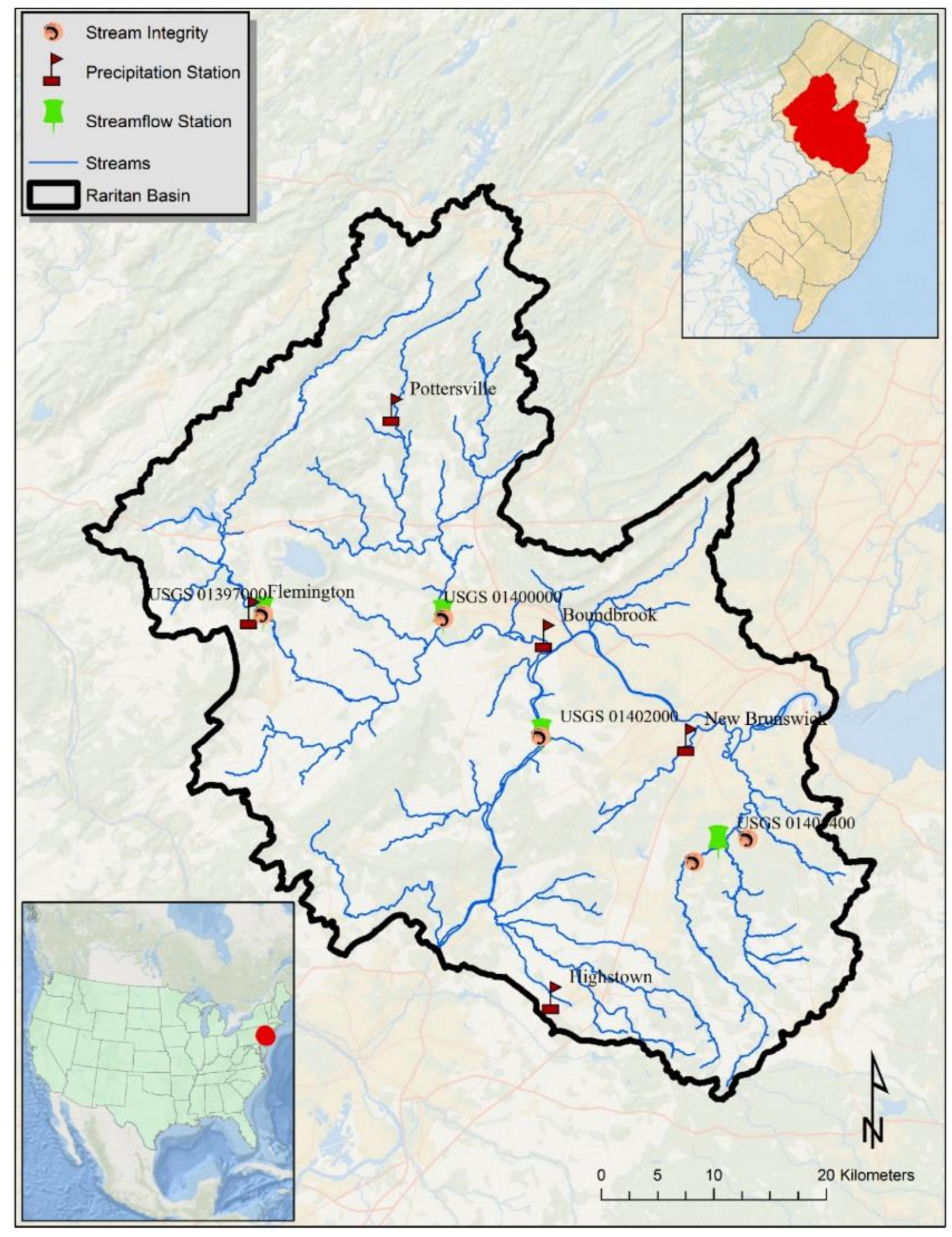
2.1. Study Area

Raritan Basin is located in north-central New Jersey (Figure 1), and it is the largest Basin located entirely within the state of New Jersey. The Basin has a total area of 2862 km² of which 43.5% is urban land, 25.3% forest, 16.0% agricultural lands, 11.8% wetlands, 2.2% water, and remaining is barren lands. North and South Branch are the two headwater rivers, and they join to form the main stem of the Raritan River. The Raritan River flows eastward and finally drains into the Atlantic Ocean. Millstone River, Green Brook, Lawrence Brook, and South River are primary tributaries to the Raritan River. Three distinct physiographic provinces, including Highlands, Piedmonts, and Coastal Plains, are found in the basin. The Highlands Provinces are located in the north of the basin, having rugged topography and discontinuous, rounded ridges separated by narrow valleys. The Piedmont regions are situated in the center of the basin and are characterized by low, rolling plains divided by higher ridges underlain by folded and faulted sedimentary and igneous rocks. The Coastal Plain is located in the southeast side of the basin, consisting of predominately unconsolidated deposits in low relief. From a meteorological standpoint, Raritan Basin has an average annual mean temperature of 17.3 °C, while the average annual minimum and maximum temperature are 15.2 °C and 19.2 °C [45]. The coldest month is January, having an average monthly temperature of 4 °C, while the hottest month is July, with an average monthly temperature of 29.7 °C. Therefore, the basin is characterized by a continental climate that consists of both hot and humid during summer and cold during winter. The average annual precipitation in the Basin varies from 1731 mm (maximum) to 776 mm (minimum) with a mean value of 1211 mm. The average annual discharge rate of Raritan River located at USGS-1403060 streamflow gauging station is 33.2 m³/sec [46], which is located approximately in the center of the Basin. Due to lack of USGS gauging station near the basin outlet, we cannot provide the Raritan River discharge draining into the Atlantic Ocean. From an ecosystems health prospective, Raritan River serves as habitat to some of the best trout fish in the state of New Jersey. Additionally, it provides a natural corridor to numerous threatened and endangered species. Furthermore, this basin provides myriad of recreational opportunities to the residents and others that increase the quality of life. Therefore, a thorough understanding of drought analysis is required to develop early warning systems to alert farmers and policymakers for timely water supply management in the basin.

2.2. Climatic and Streamflow Dataset

The meteorological drought was calculated based on the precipitation data for each meteorological station within the Raritan Basin. The precipitation data were obtained from the National Centers for Environmental Information of National Oceanic and Atmospheric Administration (NOAA). Initially, precipitation data were downloaded for all the existing stations within the study basin; however, stations having few years of precipitation data were eliminated for further analysis. Finally, five meteorological stations having 39 years (1980–2018) of daily precipitation data were selected for meteorological drought analysis (Figure 1). The hydrological drought was estimated based on the streamflow data of each USGS streamflow gauging station. Four USGS streamflow gaging stations located close to the meteorological stations were selected for this study (Figure 1). The daily streamflow of 38 years (1981–2018) was acquired for four USGS streamflow gauging stations, and further, these streamflow data were converted into average monthly streamflow. Two out of four USGS gauging stations did not have streamflow data for 1980; therefore, streamflow for all stations were downloaded from 1981 instead of 1980 in order to maintain consistency.

2.3. Computation of Meteorological and Hydrological Drought

The meteorological and hydrological drought and their severity was characterized based on SPI and SSI, respectively. SPI is one of the widely accepted meteorological drought indices. McKee et al. [16] developed SPI for characterizing drought using precipitation for a desired time period. The SPI measures precipitation deficit based on the probability distribution of precipitation at different accumulation periods. More specifically, it measures the standardized departure of observed precipitation of the desired accumulation period from its long term average precipitation [13,47,48,49]. The advantages of using SPI for drought characterization are (i) it can be calculated for different accumulation periods of interest for monitoring soil moisture (short-term precipitation deficit impact) as well as streamflow and reservoir water level (long-term precipitation deficit impact), and (ii) it considers the stochastic nature of the drought resulting in a robust measure of both short- and long-term meteorological drought [50]. The following steps were performed in order to generate SPI for different accumulation periods, including 1 month, 3 months, 6 months, and 12 months.

Step 1: A total of 39 years (1980 to 2018) of daily precipitation data for five meteorological stations (Figure 1) were collected from the National Centers for Environmental Information of National Oceanic and Atmospheric Administration (NOAA). The daily precipitation data were converted to monthly cumulative using Python Script.

Step 2: The precipitation time series of different accumulation periods, including 1 month, 3 months, 6 months, and 12 months, were fitted to a probability density function (e.g., gamma distribution). The probability density function of gamma distribution was presented as:

$$\mathrm{g}(x_k)=\frac{1}{{\beta }^{\alpha }\mathsf{\Gamma }\left(\alpha \right)}{x}_k^{\alpha -1}{e}^{-x/\beta } for x_k>0$$

(1)

where α was the shape factor, β was the scale factor, and x_k was the amount of precipitation. All parameters α, β, and x_k were positive. The gamma function Γ(α) was defined as:

$$\mathsf{\Gamma }\left(\mathsf{\alpha }\right)=\underset{0}{\overset{\infty }{\int }}{y}^{\alpha -1}{e}^{-y}dy$$

(2)

Step 3: A cumulative density function of the identified probability density function was determined, and it was transformed to standard normal distribution having mean zero and standard deviation one, which resulted into SPI. This SPI was calculated in R platform using SPEI package [51].

SSI characterizes hydrological drought by allowing accurate spatio-temporal comparison of streamflow condition in the river system [52]. The hydrological drought was characterized using SSI for different accumulation periods, including 1 month, 3 months, 6 months, and 12 months. Computation of SSI was followed the same procedure (from Step 2 of SSI) using the SPEI package in R platform.

2.4. Trend Analysis

Temporal trends (i.e., abrupt change or gradual change) in datasets can be detected using either parametric or non-parametric tests. Parametric test requires to satisfy both independence and normal distribution of dataset assumptions, whilst a non-parametric test needs to validate only the independence of data. Therefore, nonparametric methods are most widely used in the scientific communities to identify the trend and its possible implications on environment. Mann–Kendall (MK) test as well Sen’s slope (SS) were used in this study to identify monotonic trends in the hydro-climatic data.

2.4.1. Mann–Kendall Test

MK test is a nonparametric rank-based test that identifies the presence of trends in time-series data. This test was developed by Mann [53] and further improved by Kendall [54]. The null hypothesis of this test is that there is no trend in the time series, whilst the alternative hypothesis is that there is a trend. This test can handle missing data as well as irregularly spaced monitoring data. The MK test statistics is based on S value, where the positive value shows increasing trend, and the negative value depicts decreasing trend [53,54]:

The MK test was performed at 0.05 significance level (i.e., α = 0.05).

2.4.2. Sen’s Slope (SS)

The MK test provides the direction of the trend (i.e., whether the trend is increasing or decreasing); therefore, researchers use SS concomitant with MK test to assess a complete trend of a time series, as SS estimates the magnitude of the trend [6]. SS is the nonparametric test that estimates the trends of univariate time series. SS is the median of all pairwise slopes in the time series arranged in increasing order [55].

2.5. Water Quality and Stream Integrity Data

Hydrological drought can affect water quality and stream integrity through different physical, chemical, and biological processes [56]. Since hydrological drought can seriously impact some of the critical values during low flow condition, a detailed understanding of hydrological drought on water quality and stream integrity is a prerequisite for formulation of essential policy in drought-prone basins. The water quality data, including sediment, TP, TN, turbidity, and fecal coliform, were downloaded from National Water Quality Monitoring Council Portal for all four USGS streamflow gauging stations (Figure 1) between 1981 to 2018. However, all the USGS streamflow gauging stations except USGS-01397000 did not have long-term water quality data. Therefore, water quality data only from USGS-01397000 were used against the SSI index developed at this gauging station to understand the impacts of hydrological drought to stream water quality. If SSI value was lesser than equal to −0.5, it was considered as drought; otherwise, it was categorized as a non-drought event. The SSI values were classified as drought and non-drought based on the availability of water quality data of a particular month between 1981 to 2018. In case more than one water quality value was observed for a particular month, then an average water quality value was considered for that month. This process was repeated for four accumulation periods (1 month, 3 months, 6 months, and 12 months) and five water quality parameters (sediment, TP, TN, turbidity, and fecal coliform) consisting of a total of 40 scenarios (2 categories (drought and non-drought) × 4 accumulation periods × 5 water qualities). The total number of samples for sediment, TP, TN, turbidity, and fecal coliform data were 49, 75, 71, 52, and 28, respectively.

The stream integrity data were collected for three USGS streamflow gauging stations, where stream integrity sampling stations were located exactly on USGS streamflow gauging stations (Figure 1). The stream integrity data for the years 1998, 2004, 2009, and 2014 were developed by Ambient Biomonitoring Network (AMNET) of the New Jersey Department of Environmental Protection (NJDEP) for our study basin. These stream integrity data were developed based on the benthic macroinvertebrates samples collected at each station and further processed according to the NJDEP Field Procedure Manual, Rapid Bioassessment Protocol. Since collecting macroinvertebrate samples and developing stream integrity index is expensive and time consuming, only one stream integrity index per stream integrity sampling station per year was provided for this analysis. Based on the conservative approach, the SSI value of December was selected for the corresponding year of available stream integrity data as the SSI value of December and had the most severe hydrological drought in all accumulation periods except 12 months. Similar to water quality analysis, if the SSI value of December of the corresponding available stream integrity index was less than or equal to −0.5, then it was considered as drought; otherwise, it was considered as a non-drought event. The total number of samples for this analysis was 12 (3 stream integrity station × 4 years’ of stream integrity data).

To compare the mean difference of different water quality as well as stream integrity values between drought and non-drought periods, Welch’s t-test was used instead of Student’s t-test, as unequal sample sizes were observed between drought and non-drought periods. Welch’s t-test is a modification of Student’s t-test and is intended to use to determine the mean difference between two groups whenever sample sizes and unequal variance exists between two groups [57,58,59]. The α value (i.e., significance level) of 0.05 was considered for this test, and it was conducted using R platform.

3. Results and Discussion

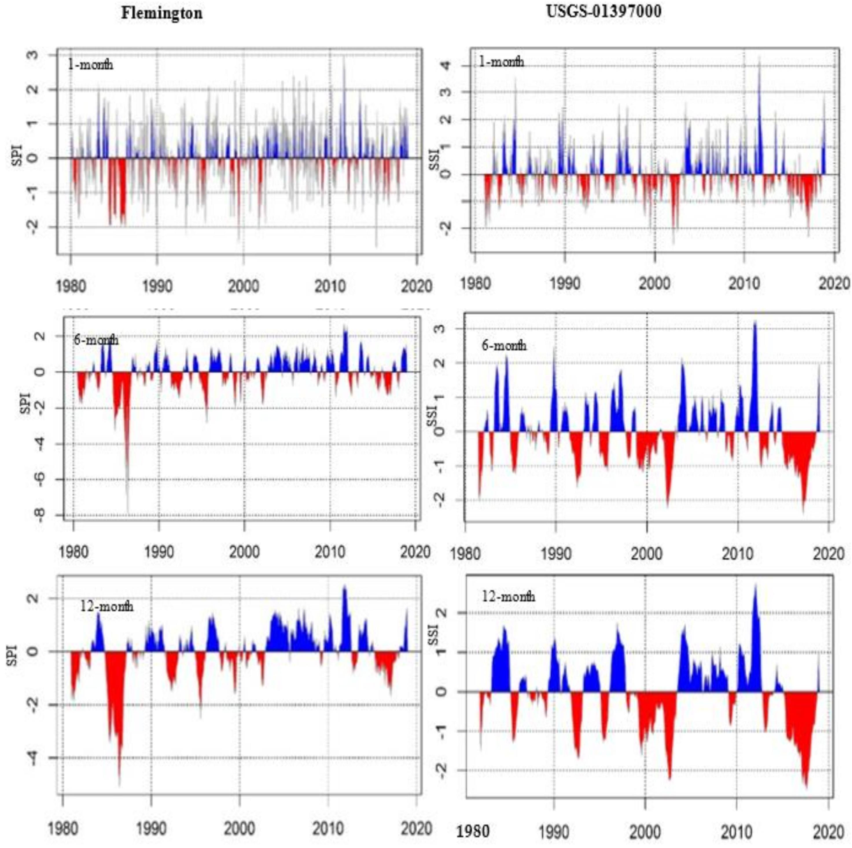
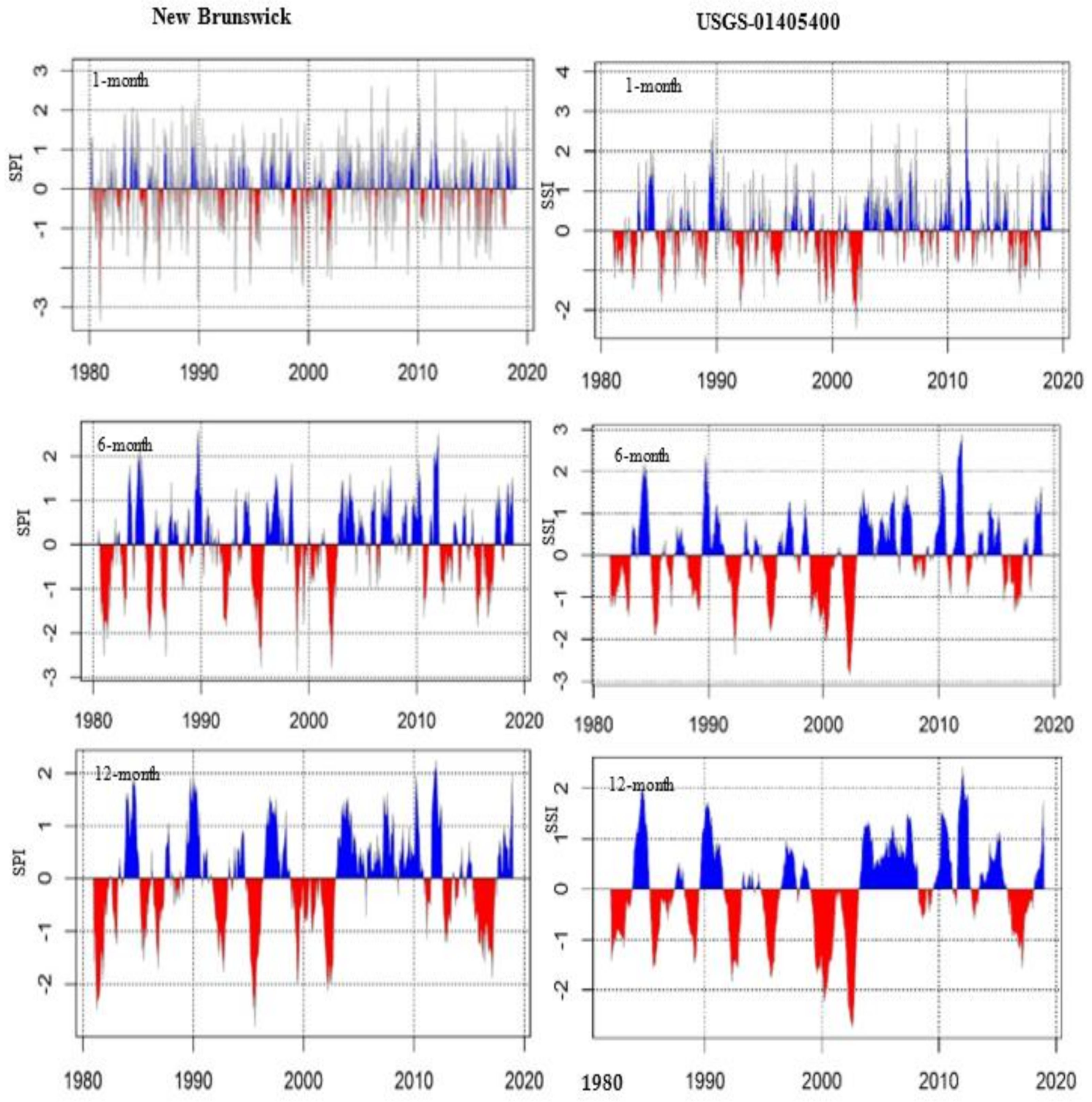
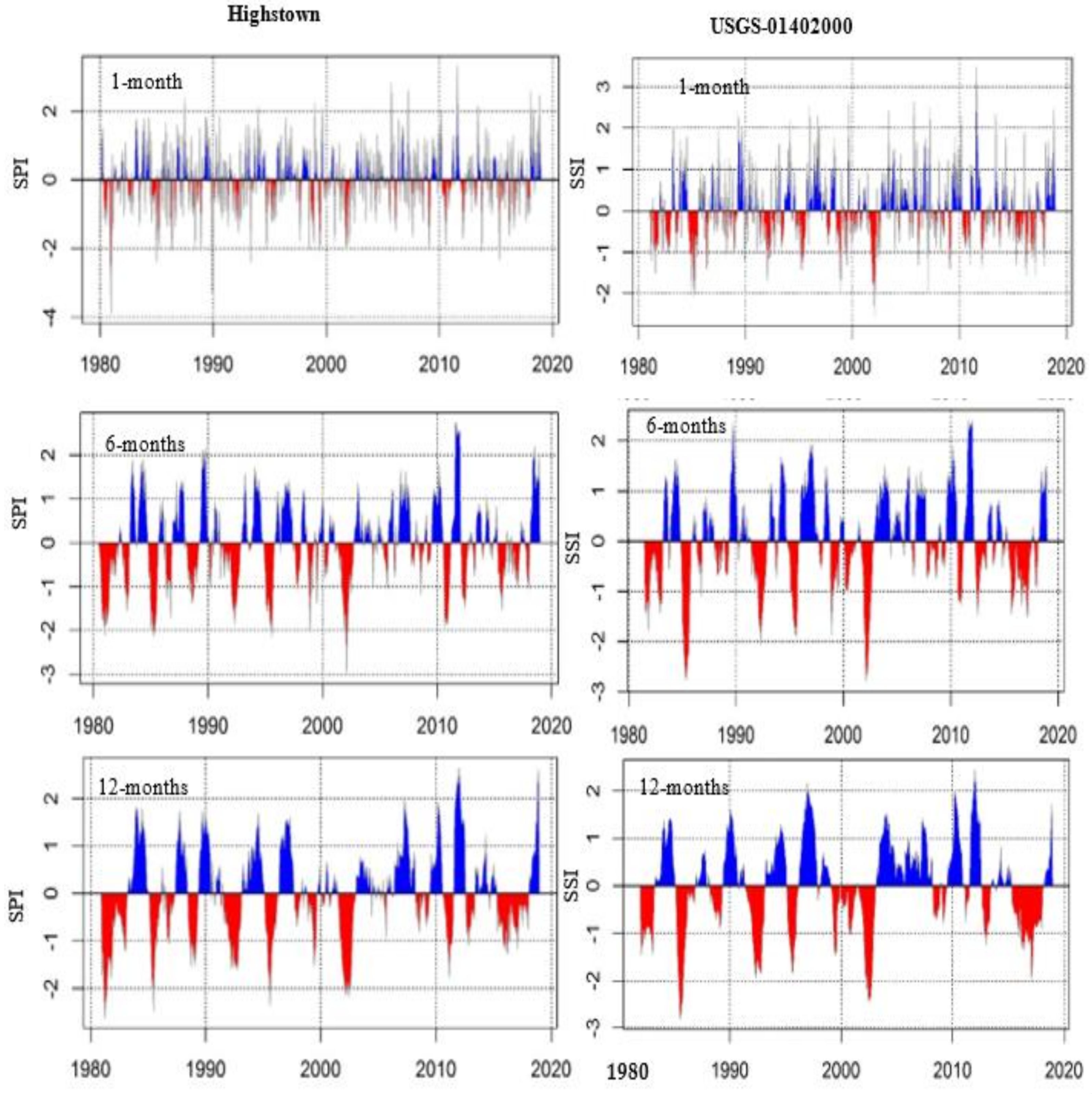
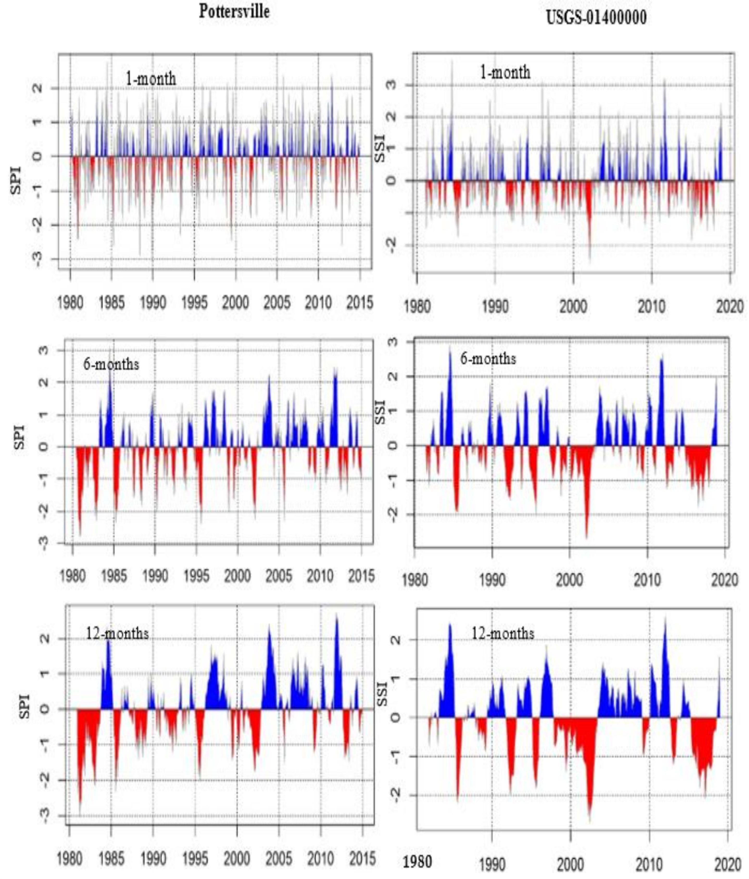
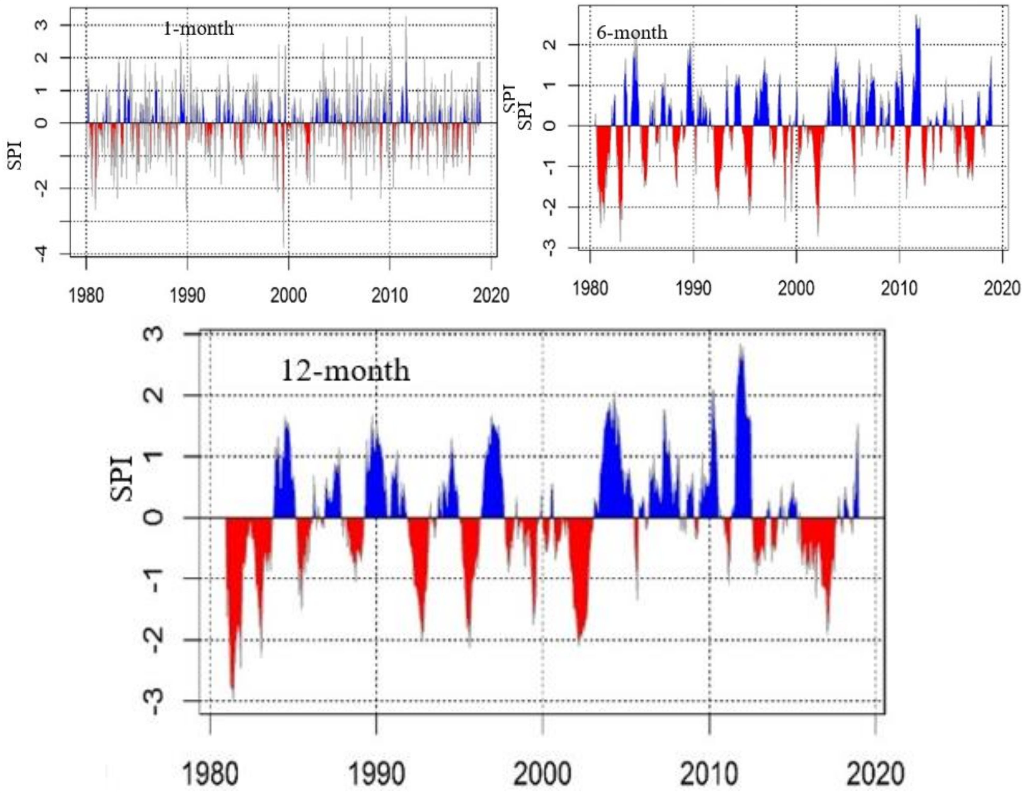
3.1. Meteorological and Hydrological Drought Temporal Evolutions and Characteristics

The temporal analysis of meteorological and hydrological drought was performed for five meteorological stations and four USGS streamflow gauging stations located within the Raritan Basin. The meteorological drought of Flemington station (western side of the basin) was compared with hydrological drought at USGS 01,397,000 streamflow gauging station located within close proximity to Flemington station (Figure 1). On the eastern side of the basin, the meteorological drought of the New Brunswick station was correlated to hydrological drought at USGS 01,405,400 streamflow gauging station. The meteorological drought in the northern part of the basin is represented by Pottersville station, and it was compared with hydrological drought at USGS 01,400,000 streamflow gauging station located downstream of the Pottersville station. The meteorological drought of Highstown station, located in the southern part of the basin, was compared to hydrological drought at USGS 01,402,000 streamflow gauging station situated downstream of the Highstown station. The Bound Brook meteorological station was analyzed only for meteorological drought due to the lack of downstream streamflow station having long-term streamflow data. The meteorological drought of all stations except Pottersville is from 1980 to 2018, whilst the hydrological drought is analyzed from 1981 to 2018. The results of the three-month accumulation periods for SPI and SSI are not presented due to similarity between one-month and three-months accumulation periods.

Both SPI and SSI are presented by three different accumulation periods, including 1 month, 6 months, and 12 months. Using a shorter accumulation period (i.e., one month), the occurrence of both dry and wet periods is more frequent, resulting in lack of any notable trend (Figure 2, Figure 3, Figure 4, Figure 5 and Figure 6). As we move from a 1-month accumulation period to 12-months, the historical drought events are more notable in the ascending order. In fact, the historical drought events are more prominent based on 6-months and 12-months accumulation periods. Therefore, the following interpretations are based on the two aforementioned accumulation periods.

It is worth noting that both wet and dry periods are presented in temporal analysis; however, only drought events are discussed in this study. At the Flemington meteorological station and its corresponding USGS streamflow gauging station, both SPI and SSI are detected the drought events of 1981 and 1982 with nearly equal magnitude, respectively (Figure 2). The next drought event identified by both indices is between 1985 and 1986. In contrast to previous events, the magnitude of SPI is higher than SSI. In fact, the magnitude of SPI is the highest during this event throughout the 39 years of drought analysis. However, the highest severity of meteorological drought does not resonate with the highest hydrological drought, as evident from both indices. This result may be because SPI is calculated solely based on precipitation data without potential evapotranspiration. One of the primary factors that plays a significant role in propagating meteorological drought to hydrological drought is evapotranspiration [4]. The exclusion of potential evapotranspiration could overestimate the SPI leading to drought severity. Byakatonda et al. [6] also observed the overestimation of SPI compared to SPEI in evaluating drought severity in Botswana, located in southern Africa. The next two mild droughts are reported by both indices in the years 1992 and 1995, showing approximately equal severity. The longest duration of drought detected in the western region in the basin is from 1998 to 2002. This continuous meteorological drought resulted in one of the highest-severity hydrological droughts in this region. Prolonged precipitation deficit results in depletion of soil moisture, lesser surface runoff into stream, and decline in groundwater recharge into streamflow, which translates into lesser streamflow and the highest severity of hydrological drought. Our finding is echoed with the Drought Emergency category declaration during 2001 and 2002 by the Division of Water Supply of New Jersey Environmental Protection, which focused on reducing water demands [60]. The most recent drought event was on April 2015, and its departure was observed at end of 2017. Both indicators can identify drought during this period, but SSI shows a higher degree of severity.

On the east side of the basin at New Brunswick station, the drought events of 1981 and 1982 detected in the westside (at Flemington station) are also observed (Figure 3). However, SPI is slightly higher compared to the westside. When SPI is compared with the SSI of this station, higher SPI magnitude is noted compared to SSI. Another salient feature is noticed in the onset and departure of SPI and SSI. Even though both meteorological and hydrological drought started nearly simultaneously, the departure of hydrological drought took a bit longer compared to meteorological drought. The drought recorded during 1985 and 1986 on the westside was also observed at this station. However, the magnitude of the meteorological drought is much higher on the west side compared to this station. One of the reasons that could explain this slightly higher meteorological drought in the west side compared to this station is the location of both stations.

The western-side station is located in the northern climate zone, while this station is located in the central climate zone [61]. While both stations have a continental climate, the westside station has minimal influence from the Atlantic Ocean compared to this station. When SPI and SSI are compared for this station, an approximately equal amount of magnitude is observed. The 1992 and 1995 mild drought events detected in the west side are also reported at this station by both indices. When the magnitude of SPI at the west side and this station are compared, both have nearly equal magnitude. Similar results are also found when compared with SSI of the west side and this station. A prolonged meteorological drought (similar to westside) was observed at this station during 1998 and 2002, and this prolonged meteorological drought translated into the highest magnitude of hydrological drought.

However, the onset of both droughts at this station is late compared to the west side. The most recent meteorological drought event that occurred at this station was from mid of 2015 to mid of 2017. However, the hydrological drought started at this station was from the end of 2015 to the end of 2017. Compared to the west side, the meteorological drought departure was early at this station. This early departure of meteorological drought at this station also results into lesser magnitude of hydrological drought compared to the west side.

In the south at Highstown (Figure 4) and in the north at Pottersville (Figure 5), all the meteorological and hydrological drought events observed in the previous two stations are also detected at these stations nearly in equal magnitude. The meteorological drought at Bound Brook (Figure 6) captured all the meteorological drought events observed in other stations in the basin. Overall, both indices are able to identify each of the historical drought events that occurred during the study period with approximately equal magnitude in most of the events. These two indices are able to detect all three drought emergency periods (1981, 1985, and 2001–2002) as well as most recent drought-watch periods (2015 and 2016) in the basin, demonstrating that both indices can be used by policymakers and practitioners for drought forecasting and management strategies based on the future climate change.

For each accumulation period and station, drought event, mean duration, and mean severity were calculated based on the threshold −0.5 to −1.49 (moderate drought), −1.5 to −1.99 (severe drought), and −2 (extreme drought) both for meteorological and hydrological droughts (

Table 1. Meteorological drought characterization (severity and duration) using SPI for Raritan Basin.

Station	Threshold	Accumulation Period (Months)	Total Number of Drought Events	Mean Duration (Months)	Mean Severity
Flemington	−0.5 to −1.49	1	70	1	−1.31
		3	58	2	−1.54
		6	35	3	−2.50
		12	24	3	−3.06
	−1.5 to −1.99	1	17	2	−3.00
		3	13	3	−3.27
		6	13	2	−2.41
		12	7	3	−2.97
	≤−2.0	1	4	1	−2.33
		3	5	2	−5.50
		6	6	3	−9.23
		12	3	7	−22.72
New Brunswick	−0.5 to −1.49	1	89	1	−1.14
		3	56	2	−1.87
		6	47	2	−2.05
		12	38	3	−2.49
	−1.5 to −1.99	1	12	1	−1.78
		3	15	1	−1.69
		6	14	2	−1.71
		12	17	1	−1.71
	≤−2.0	1	13	1	−2.31
		3	5	1	−2.35
		6	6	1	−2.19
		12	5	2	−2.27
Highstown	−0.5 to −1.49	1	82	1	−1.12
		3	55	2	−1.93
		6	39	2	−2.06
		12	30	4	−3.31
	−1.5 to −1.99	1	16	1	−1.80
		3	16	1	−1.93
		6	20	2	−2.64
		12	13	2	−2.97
	≤−2.0	1	14	1	−2.87
		3	9	1	−3.00
		6	7	1	−3.55
		12	3	3	−7.69
Pottersville	−0.5 to −1.49	1	68	1	−1.17
		3	60	2	−1.56
		6	42	2	−1.83
		12	30	3	−2.92
	−1.5 to −1.99	1	23	1	−1.76
		3	15	1	−1.86
		6	15	1	−2.25
		12	10	2	−2.70
	≤−2.0	1	8	1	−3.10
		3	11	1	−2.74
		6	10	1	−2.99
		12	5	2	−4.73
Bound Brook	−0.5 to −1.49	1	76	1	−1.22
		3	56	2	−1.66
		6	45	2	−1.99
		12	32	3	−2.75
	−1.5 to −1.99	1	24	1	−1.80
		3	16	1	−2.02
		6	17	1	−2.30
		12	12	2	−3.53
	≤−2.0	1	9	1	−2.50
		3	11	1	−3.08
		6	10	1	−2.99
		12	6	2	−3.97

and

Table 2. Hydrological drought characterization (severity and duration) using SSI for Raritan Basin.

Station	Threshold	Accumulation Period (Months)	Total Number of Drought Events	Mean Duration (Months)	Mean Severity
USGS−01397000	−0.5 to −1.49	1	70	2	−1.49
		3	35	3	−2.88
		6	23	5	−5.89
		12	14	7	−6.89
	−1.5 to −1.99	1	9	1	−1.69
		3	6	2	−3.12
		6	7	1	−2.20
		12	8	3	−4.13
	≤−2.0	1	5	1	−2.23
		3	2	2	−4.66
		6	4	3	−5.26
		12	2	7	−14.51
USGS−01405400	−0.5 to −1.49	1	69	2	−1.51
		3	34	3	−2.91
		6	21	5	−4.61
		12	21	4	−4.24
	−1.5 to −1.99	1	11	1	−1.74
		3	10	1	−1.72
		6	10	2	−1.72
		12	11	2	−1.66
	≤−2.0	1	2	1	−2.43
		3	4	3	−6.24
		6	3	3	−7.25
		12	2	5	−12.00
USGS−01402000	−0.5 to −1.49	1	73	2	−1.468
		3	46	3	−2.39
		6	34	3	−2.79
		12	20	5	−4.80
	−1.5 to −1.99	1	9	1	−1.93
		3	9	1	−2.46
		6	10	2	−3.07
		12	9	2	−4.14
	≤−2.0	1	3	1	−2.48
		3	2	5	−10.36
		6	3	4	−9.09
		12	3	4	−8.82
USGS−01400000	−0.5 to −1.49	1	70	2	−1.66
		3	45	3	−2.56
		6	33	4	−3.36
		12	24	5	−4.33
	−1.5 to −1.99	1	5	1	−2.02
		3	6	2	−3.07
		6	7	2	−3.75
		12	11	2	−2.85
	≤−2.0	1	1	1	−2.59
		3	1	3	−7.4
		6	1	5	−12.11
		12	4	3	−6.25

). As expected, the total number of drought events are highest for shorter accumulation periods and thresholds closer to zero. As the accumulation period as well as threshold increases, the mean duration and severity of drought also intensifies.

3.2. Trend Analysis of Meteorological and Hydrological Drought

Trend analysis of meteorological and hydrological drought of different accumulation periods, such as 1 month, 3 months, 6 months, and 12 months, were performed using MK test, and the results are presented in

Table 3. Mann–Kendall test for meteorological drought in Raritan Basin.

Station	SPI	Kendall’s Tau	p Value	Sen’s Slope	Trend
Bound Brook	SPI-1	0.034	0.275	0	NS
	SPI-3	0.045	0.151	0.001	NS
	SPI-6	0.047	0.130	0.001	NS
	SPI-12	0.069	0.027 *	0.001	S
Flemington	SPI-1	0.085	0.006 *	0.001	S
	SPI-3	0.1	0.001 *	0.001	S
	SPI-6	0.132	0.000 *	0.002	S
	SPI-12	0.165	0.000 *	0.002	S
Highstown	SPI-1	0.036	0.249	0	NS
	SPI-3	0.049	0.121	0.001	NS
	SPI-6	0.054	0.087	0.001	NS
	SPI-12	0.064	0.041 *	0.001	S
New Brunswick	SPI-1	0.041	0.182	0	NS
	SPI-3	0.053	0.089	0.001	NS
	SPI-6	0.058	0.062	0.001	NS
	SPI-12	0.033	0.283	0	NS
Pottersville	SPI-1	0.03	0.327	0	NS
	SPI-3	0.052	0.095	0.001	NS
	SPI-6	0.051	0.102	0.001	NS
	SPI-12	0.118	0 *	0.002	S

NS, not significant, and S, significant, at 5% level of significance while * represents statistically significant at 5% level of significance.

and

Table 4. Mann–Kendall test for hydrological drought in Raritan Basin.

Station	SPI	Kendall’s Tau	p Value	Sen’s Slope	Trend
USGS-01397000	SSI-1	−0.030	0.345	0	NS
	SSI-3	−0.087	0.006 *	−0.001	S
	SSI-6	−0.100	0.002 *	−0.001	S
	SSI-12	−0.111	0.001 *	−0.001	S
USGS-01402000	SSI-1	0.048	0.122	0	NS
	SSI-3	0.018	0.563	0	NS
	SSI-6	0.012	0.713	0	NS
	SSI-12	0.020	0.528	0	NS
USGS-01405400	SSI-1	0.053	0.088	0.001	NS
	SSI-3	0.077	0.015 *	0.001	S
	SSI-6	0.094	0.003 *	0.001	S
	SSI-12	0.116	0.000 *	0.001	S
USGS-01400000	SSI-1	0.013	0.677	0	NS
	SSI-3	−0.022	0.487	0	NS
	SSI-6	−0.052	0.102	−0.001	NS
	SSI-12	−0.063	0.048 *	−0.001	S

NS, not significant, and S, significant, at 5% level of significance while * represents statistically significant at 5% level of significance.

, respectively. Out of five meteorological stations, only Flemington showed significant positive meteorological drought trend for all accumulation periods. Both p-values of Kendall’s Tau and Sen’s slope agree with each other, having significant positive meteorological drought trend for Flemington at 5% level of significance (Table 3). This indicates that the western part of the Raritan basin is susceptible to meteorological drought. This part belongs to the highlands and valley region, and the major sources of precipitation are from storm tracks extending from the Mississippi Valley, Great Lakes, and St. Lawrence Valley [62]. By the time the storm track travels from the aforementioned locations to the western part of the basin, it becomes weaker, leading to lesser precipitation. Additionally, this part of the basin has minimal influence from the Atlantic Ocean. High susceptibility to meteorological drought in the western part of the basin, particularly at Flemington station, can lead to severe consequences to the water supply in the state of New Jersey, as the Round Valley Reservoir (the largest reservoir in the state) is situated closer to this station, and this reservoir serves a major source of water supply in the central New Jersey area.

In contrast to Flemington station, the New Brunswick station showed insignificant positive meteorological drought trends for all accumulation periods at 5% level of significance (Table 3). This trend is verified by both p-values of Kendall’s Tau as well as Sen’s slope. The insignificant drought trend is primarily due to higher precipitation due to maximum influence from the Atlantic Ocean. The remaining stations, including Bound Brook, Highstown, and Pottersville, do not depict a significant positive drought trend at 5% level of significance for all accumulation periods except 12 months. When the meteorological drought trend is compared among different accumulation periods, only SPI-12 shows a significant positive trend in most of the stations inside the basin. This indicates that most parts of the basin (except the western side) have no less than average precipitation for long time periods.

The hydrological drought of different accumulation periods, including 1 month, 6 months, and 12 months, are presented in Table 4. USGS-01397000 streamflow gauging station shows a significant negative hydrological drought trend, whilst the USGS-01405400 streamflow gauging station depicts significant positive trend at 5% level of significance for all accumulation periods except SSI-1. The negative trend at USGS-01397000 streamflow gauging station shows a positive sign for water supply and ecosystem health, whilst the positive hydrological drought sign at USGS-01405400 streamflow gauging station may have serious negative impacts. USGS-01402000 streamflow gauging station demonstrates no trend for all accumulation periods, as the Sen’s slope is 0, whilst USGS-01400000 streamflow gauging station exhibits no trend only for SSI-1 and SSI-3. When the trends of meteorological drought of each station are compared with the hydrological drought of corresponding USGS streamflow gauging station, all stations except Flemington show a similar trend. A positive meteorological drought trend is observed at Flemington station, whilst a significant negative hydrological drought trend is assessed at its corresponding USGS streamflow station (USGS-01397000). This demonstrates the impacts of anthropogenic activities, such as change in land use (i.e., formation of new forested areas in this region in the basin). Ilstedt et al. [63] highlighted an increase in groundwater recharge through increasing tree cover in West Africa. Increased groundwater contributes to streamflow during the drought periods. Overall, the trend analysis of both meteorological and hydrological droughts depicts a significant positive or negative trend at a longer accumulation period (i.e., 12 months), whilst the shortest accumulation period (1 month) shows insignificant trends.

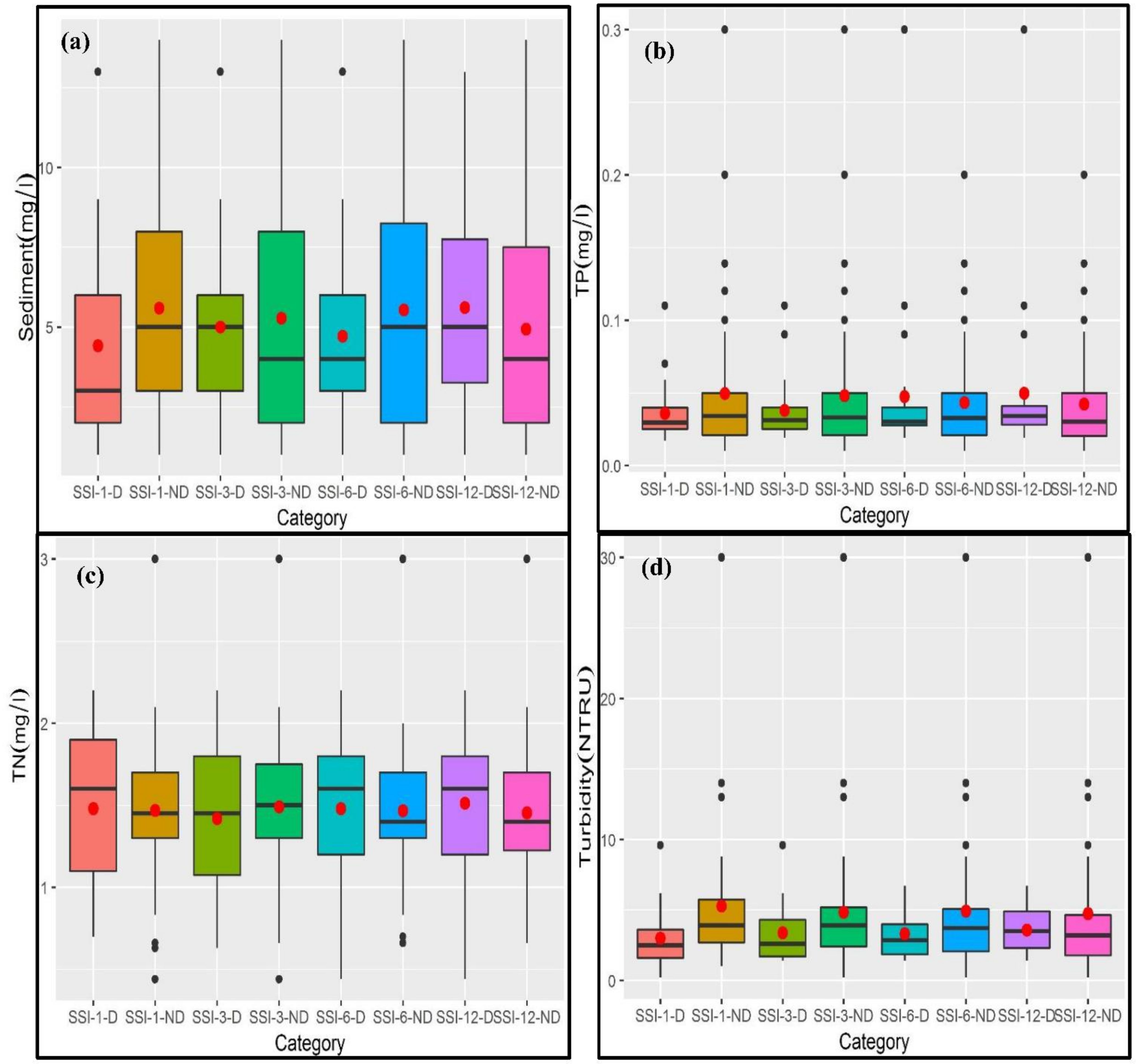
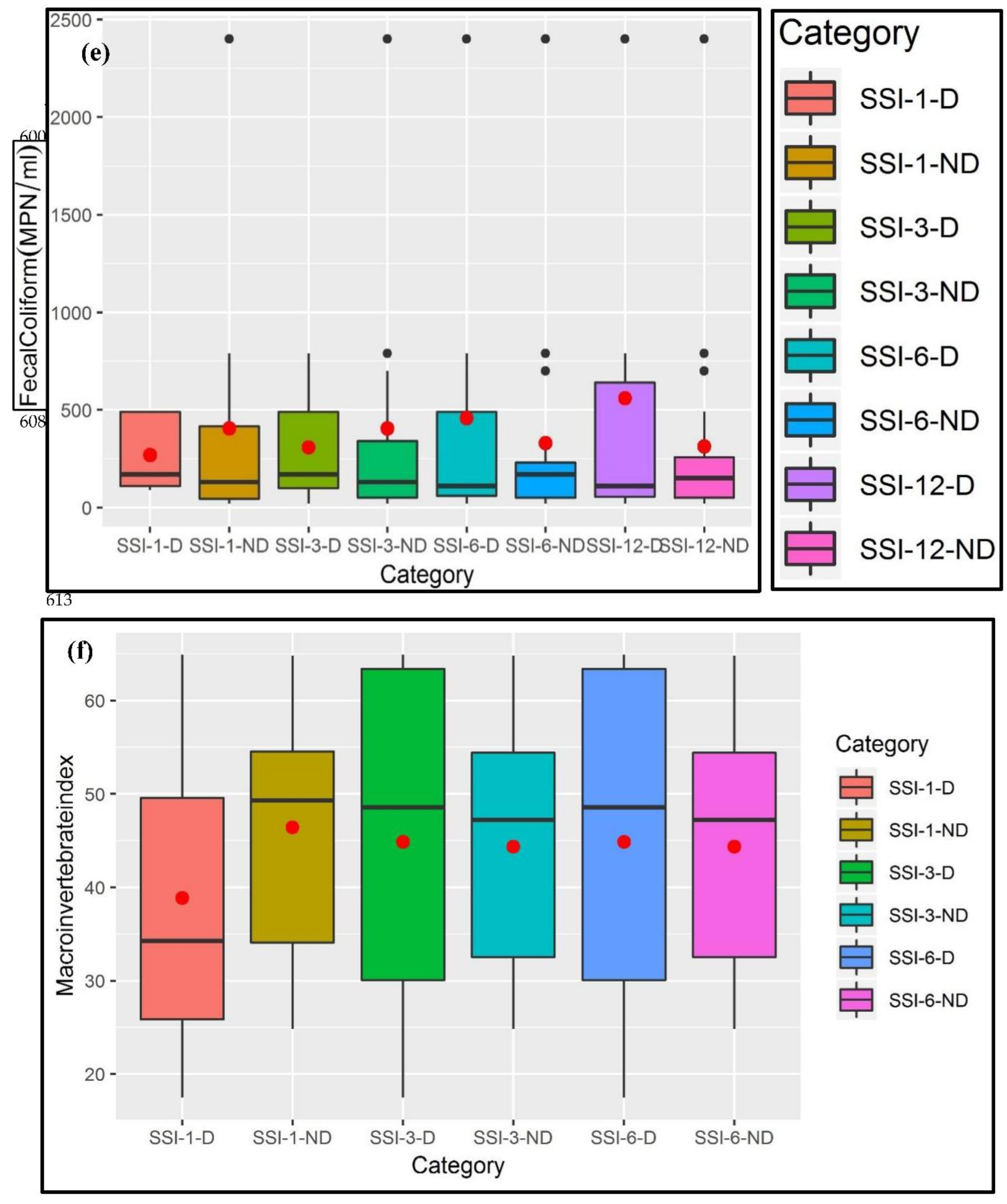
3.3. Understanding the Impacts of Hydrological Droughts and Non-Droughts on Water Quality and Stream Integrity

Out of four USGS streamflow gauging stations, USGS-01397000 has the highest amount of water quality data available, and it is located in close proximity to a meteorological station (i.e., Flemington). Therefore, USGS-01397000 streamflow gauging station is selected for understanding the impacts of hydrological drought and non-drought on various water quality parameters, including sediment, total phosphorus, total nitrogen, turbidity, and fecal coliform.

The water quality trend between drought and non-drought of different accumulation periods for sediment and total phosphorus demonstrates a similar pattern (Figure 7a,b). The mean pollutant concentration of the drought period is lesser than the non-drought period. As we move from SSI-1 to SSI-6, the difference between drought and non-drought period gradually decreases, and finally, during SSI-12, the mean pollutant concentration of drought period becomes greater than the non-drought period. This trend can be further verified from Welch’s t-test between drought and non-drought periods (

Table 5. Welch’s t-test for water quality parameters and stream integrity between drought and non-drought period at Flemington station.

Parameter	Group Name	Mean1 (Drought)	Mean 2 (Non-Drought)	Df	t-Stat	p-Value
Sediment	SSI-1-Drought vs. Non-Drought	4.412	5.594	35.400	−1.182	0.245
	SSI-3-Drought vs. Non-Drought	5.000	5.273	35.383	−0.275	0.785
	SSI-6-Drought vs. Non-Drought	4.714	5.536	46.697	−0.851	0.399
	SSI-12-Drought vs. Non-Drought	5.611	4.935	41.846	0.697	0.489
TP	SSI-1-Drought vs. Non-Drought	0.036	0.050	68.286	−1.664	0.101
	SSI-3-Drought vs. Non-Drought	0.038	0.048	72.678	−1.210	0.230
	SSI-6-Drought vs. Non-Drought	0.048	0.043	39.359	0.367	0.716
	SSI-12-Drought vs. Non-Drought	0.050	0.042	34.152	0.613	0.544
TN	SSI-1-Drought vs. Non-Drought	1.479	1.468	35.454	0.097	0.923
	SSI-3-Drought vs. Non-Drought	1.420	1.491	31.440	−0.598	0.554
	SSI-6-Drought vs. Non-Drought	1.480	1.466	43.629	0.127	0.899
	SSI-12-Drought vs. Non-Drought	1.513	1.454	33.960	0.502	0.619
Turbidity	SSI-1-Drought vs. Non-Drought	3.005	5.277	41.191	−2.095	0.04241 *
	SSI-3-Drought vs. Non-Drought	3.382	4.834	49.066	−1.397	0.169
	SSI-6-Drought vs. Non-Drought	3.322	4.909	43.480	−1.562	0.126
	SSI-12-Drought vs. Non-Drought	3.571	4.743	45.580	−1.167	0.250
Fecal Coliform	SSI-1-Drought vs. Non-Drought	270.000	405.304	22.617	−0.807	0.428
	SSI-3-Drought vs. Non-Drought	308.571	405.333	24.545	−0.519	0.609
	SSI-6-Drought vs. Non-Drought	458.182	331.294	18.637	0.503	0.621
	SSI-12-Drought vs. Non-Drought	551.250	313.100	9.663	0.777	0.456
Stream Integrity	SSI-1-Drought vs. Non-Drought	38.8721	46.4100	2.5136	−0.5125	0.6499
	SSI-3-Drought vs. Non-Drought	44.8675	44.3575	4.1817	0.0406	0.9695
	SSI-6-Drought vs. Non-Drought	44.8675	44.3575	4.1817	0.0406	0.9695

Note: * represents statistically significant at 5% level of significance.

). Although a difference of magnitude in sediment and total phosphorus concentration is observed between the drought and non-drought period, this differences are not statistically significant, at 5% level of significance.

One possible explanation may be due to the maximum occurrence of mild drought, which may not effectively translate into a significant difference in water quality concentration. Overall, aforementioned pollutant concentration is lower during drought periods as compared to non-drought periods. The most plausible reason is due to reduction of catchment processes as a result of reduced surface runoff, which is the primary mode of sediment and nutrient transport. This results in decreasing nonpoint source pollution delivery into rivers and streams during drought periods as opposed to non-drought periods. Van Vliet and Zwolsman [43] also observed reduced sediment concentration at Eijsden during drought condition in the Meuse River Basin, western Europe. Similar to our total phosphorus trend, Mosley et al. [64] also observed a lower concentration of total phosphorus during drought as compared to the reference period in the Lower Murray River in Australia. Aforementioned study results further substantiate our study outcomes that rivers and streams are more resilient to drought phenomenon in terms of water quality (sediment and total phosphorus).

It is worth noting that the sediment and total phosphorus concentration show greater variability for non-drought period as opposed to drought period due to presence of a greater sample size for the non-drought period compared to drought period. In case of total nitrogen, a similar trend as found for sediment and total phosphorus is observed (Figure 7c). However, the mean concentration of total nitrogen during the drought period surpasses the mean total nitrogen concentration of the non-drought period from SSI-6 (i.e., 6-months accumulation period rather than only for 12-months accumulation period, as found for sediment and total phosphorus). The Welch’s t-test also demonstrates that the drought does not have significant impacts on total nitrogen concentration as compared to non-drought period at 5% level of significance.

The relationship of turbidity to drought and non-drought period depicts a different trend as compared to trends observed in aforementioned water quality parameters (sediment, total phosphorus, and total nitrogen). The average mean turbidity is always higher in non-drought periods compared to drought periods for all accumulation periods (i.e., 1 month, 3 months, 6 months, and 12 months) (Figure 7d). In fact, the turbidity of SSI-1 during non-drought periods was significantly higher than the turbidity of drought periods at 5% level of significance (Table 5). The decreasing trend of turbidity during drought periods in rivers and streams is due to disruption of catchment processes, such as reduction of soil erosion in the landscape due to lesser precipitation as well as lesser stream bank and streambed erosion due to lack of turbulent stream velocity. Further, the increased influence of internal catchment processes, including lack of surface runoff and sedimentation during drought periods, decreases turbidity significantly in the rivers and streams. A similar pattern of lower turbidity level has been observed in other rivers during drought periods. Mosley et al. [55] observed that the turbidity level during low flow conditions was half of the turbidity level during the reference period at both sites in the Lower Murray River in Australia. Their trend was attributed to reduced river volume and mean depth of water level in conjunction with reduced sediment delivery from landscape into the river system.

The average mean concentration of fecal coliform during drought and non-drought shows a mixed trend among four accumulation periods (Figure 7e). The accumulation periods of one month and three months demonstrate a higher concentration of fecal coliform than drought periods, whilst the aforementioned trend is revered for accumulation periods of 6-months and 12-months. The higher fecal coliform concentration during drought periods compared to non-drought periods may be due to (i) greater use of river and stream water by livestock and wildlife and (ii) lack of dilution of concentration due to lesser streamflow. Overall, the difference in water quality between drought and non-drought is distinctly visible for the shortest accumulation period (i.e., one month).

The average mean of stream integrity index is higher for non-drought periods compared to drought periods for one-month accumulation period. However, no significant difference of mean stream integrity is observed between the two groups based on Welch’s t-test at 5% level of significance (Table 5). Lesser stream integrity index during drought periods compared to non-drought periods is due to reduction of streamflow as well as loss of surface water and connectivity. As the accumulation period increases, the mean differences of stream integrity between the two groups becomes approximately zero.

4. Conclusions

Understanding the drought evolution and characteristics through an index-based approach is an effective tool for assessing the adverse impacts of droughts on water resources, agriculture, hydrology, water quality, and ecosystems. This study attempts to characterize historical meteorological and hydrological droughts for various accumulation periods, including 1 month, 3 months, 6 months, and 12 months, through standardized precipitation index (SPI) and standardized streamflow index (SSI), respectively, in the Raritan Basin. The monotonic trends of aforementioned droughts were evaluated using the Mann-Kendall test and Sen’s slope estimator. Further, the impacts of hydrological droughts and non-droughts on water quality, including total phosphorus (TP), total nitrogen (TN), turbidity, and fecal coliform, as well as stream integrity were assessed. This study is the first comprehensive study in the state of New Jersey that characterizes both meteorological and hydrological droughts for a long-term period (i.e., approximately 39 years). Based on this study, the following conclusions can be inferred:

• Both SPI and SSI were able to identify historical drought events, including three drought emergency periods (1981, 1985, and 2001–2002), as well as the most recent drought-watch periods (2015 and 2016) in the basin. This demonstrates that both indices can be used to monitor future droughts events and develop early warning systems in the Basin. Out of all accumulation periods, historical drought events were prominent and notable based on 6-months and 12-months accumulation periods.
• A significant positive meteorological drought trend was observed at the western side of the basin due to weaker storm track concomitant with minimal influence from the Atlantic Ocean. However, the impacts of meteorological drought were not translated into hydrological drought, which may be due to change in land cover (i.e., increase in forest cover). In the meantime, an increasing hydrological drought trend was observed in the eastern side of the Basin. This may be due to anthropogenic activities, such as withdrawal of water from the river for different purposes, as more urban areas are located in the eastern part of the Basin. Overall, a distinct increasing/decreasing trend was observed only in 12-months accumulation period both for meteorological and hydrological droughts.
• A clear trend between drought and non-drought period was observed only for the one-month accumulation period, where the mean pollutant concentration of the drought period was less than the non-drought period. Reduction of different processes, such as erosion and transport of sediment and nutrients into rivers and streams due to the reduction of surface runoff in the landscape during drought periods as opposed to non-drought periods, resulted in this type of trend.
• Lower stream integrity index values were observed during drought periods compared to non-drought periods, as measured for the one-month accumulation period, due to reduction of streamflow as well as loss of surface water and connectivity during drought period.

References

1. Esfahanian, E.; Nejadhashemi, A.P.; Abouali, M.; Adhikari, U.; Zhang, Z.; Daneshvar, F.; Herman, M.R. Development and evaluation of a comprehensive drought index. J. Environ. Manag. 2017, 185, 31–43. [Google Scholar] [CrossRef] [PubMed] [Green Version]
2. Kang, H.; Sridhar, V. Assessment of Future Drought Conditions in the Chesapeake Bay Watershed. JAWRA J. Am. Water Resour. Assoc. 2017, 54, 160–183. [Google Scholar] [CrossRef]
3. Marini, G.; Fontana, N.; Mishra, A.K. Investigating drought in Apulia region, Italy using SPI and RDI. Theor. Appl. Clim. 2018, 137, 383–397. [Google Scholar] [CrossRef]
4. Van Loon, A.F. Hydrological drought explained. Wiley Interdiscip. Rev. Water 2015, 2, 359–392. [Google Scholar] [CrossRef]
5. Lioyd-Hughes, B. The impracticality of a universal drought definition. Theor. Appl. Climatol. 2014, 117, 607–611. [Google Scholar] [CrossRef] [Green Version]
6. Byakatonda, J.; Parida, B.; Moalafhi, D.B.; Kenabatho, P.K. Analysis of long term drought severity characteristics and trends across semiarid Botswana using two drought indices. Atmos. Res. 2018, 213, 492–508. [Google Scholar] [CrossRef]
7. Mukherjee, S.; Mishra, A.; Trenberth, K.E. Climate Change and Drought: A Perspective on Drought Indices. Curr. Clim. Chang. Rep. 2018, 4, 145–163. [Google Scholar] [CrossRef]
8. Mukherjee, S.; Mishra, A.K. Increase in Compound Drought and Heatwaves in a Warming World. Geophys. Res. Lett. 2021, 48. [Google Scholar] [CrossRef]
9. Kogan, F.; Guo, W.; Yang, W. Near 40-year drought trend during 1981–2019 earth warming and food security. Geomat. Nat. Hazards Risk 2020, 11, 469–490. [Google Scholar] [CrossRef]
10. McCabe, G.J.; Wolock, D.M. Variability and trends in global drought. Earth Space Sci. 2015, 2, 223–228. [Google Scholar] [CrossRef]
11. Song, X.; Song, Y.; Chen, Y. Secular trends of flobal drought since 1950. Environ. Res. Lett. 2020, 15, 094073. [Google Scholar] [CrossRef]
12. Mishra, A.K.; Singh, V.P. A review of drought concepts. J. Hydrol. 2010, 391, 202–216. [Google Scholar] [CrossRef]
13. Bayissa, Y.; Maskey, S.; Tadesse, T.; Andel, S.J.V.; Moges, S.; Griensven, A.V.; Solomatine, D. Comparison of the performance of six drought indices in characterizing historical drought for the upper Blue Nile Basin, Ethiopia. Geosciences 2018, 8, 81. [Google Scholar] [CrossRef] [Green Version]
14. Rajsekhar, D.; Singh, V.P.; Mishra, A.K. Integrated drought causality, hazard, and vulnerability assessment for future socioeconomic scenarios: An information theory perspective. J. Geophys. Res. Atmos. 2015, 120, 6346–6378. [Google Scholar] [CrossRef]
15. Wilhite, A.; Svoboda, D.; Hayes, J. Understanding the complex impacts of drought: A key to enhancing drought mitigation and preparedness. Water Resour. Manag. 2007, 21, 763–774. [Google Scholar] [CrossRef] [Green Version]
16. McKee, T.B.; Doesken, N.J.; Kleist, J. The relationship of drought frequency and duration to time scales. In Proceedings of the 8th Conference on Applied Climatology, Anaheim, CA, USA, 17–22 January 1993; American Meteorological Society: Boston, MA, USA, 1993; Volume 17, pp. 179–183. [Google Scholar]
17. McKee, T.B.; Doesken, N.J.; Kleist, J. Drought Monitoring with Multiple Time Scales. In Proceedings of the 9th Conference on Applied Climatology, Dallas, TX, USA, 15–20 January 1995; American Meteorological Society: Boston, MA, USA, 1995. [Google Scholar]
18. Edwards, D.C.; McKee, T.B. Characteristics of 20th Century Drought in the United States at Multiple Time Scales; Climo Report 97-2; Department of Atmospheric Science, Colorado State University: Fort Collins, CO, USA, 1997. [Google Scholar]
19. Palmer, W.C. Meteorologic Drought; Research Paper No. 45; US Department of Commerce, Weather Bureau: Washington, DC, USA, 1965; p. 58. [Google Scholar]
20. Alley, W.M. Palmer drought severity index: Limitations and assumptions. J. Clim. Appl. Meteorol. 1984, 23, 1100–1109. [Google Scholar] [CrossRef] [Green Version]
21. Karl, T.R. The Sensitivity of the Palmer Drought Severity Index and Palmer’s Z-Index to their Calibration Coefficients Including Potential Evapotranspiration. J. Clim. Appl. Meteorol. 1986, 25, 77–86. [Google Scholar] [CrossRef] [Green Version]
22. Vicente-Serrano, S.M.; Beguería, S.; Lopez-Moreno, I. A Multiscalar Drought Index Sensitive to Global Warming: The Standardized Precipitation Evapotranspiration Index. J. Clim. 2010, 23, 1696–1718. [Google Scholar] [CrossRef] [Green Version]
23. Gibbs, W.J.; Maher, J.V. Rainfall deciles as drought indicators. Aust. Bureau Meteorol. Bull. 1967, 48, 37. [Google Scholar]
24. Modarres, R. Streamflow drought time series forecasting. Stoch. Environ. Res. Risk Assess. 2007, 21, 223–233. [Google Scholar] [CrossRef]
25. Wang, Y.; Duan, L.; Liu, T.; Li, J.; Feng, P. A Non-stationary Standardized Streamflow Index for hydrological drought using climate and human-induced indices as covariates. Sci. Total Environ. 2020, 699, 134278. [Google Scholar] [CrossRef]
26. Shafer, B.A.; Dezman, L.E. Development of a surface water supply index (SWSI) to assess the severity of drought conditions in snowpack runoff areas. In Proceedings of the Western Snow Conference, Reno, NV, USA, 20–23 April 1982; Colorado State University: Fort Collins, CO, USA, 1982; pp. 164–175. [Google Scholar]
27. Doesken, N.J.; McKee, T.B.; Kleist, J. Development of a Surface Water Supply Index for the Western United States; Climo Report 91-3; Department of Atmospheric Science, Colorado State University: Fort Collins, CO, USA, 1991; p. 80. [Google Scholar]
28. Huang, J.; van den Dool, H.M.; Georgarakos, K.P. Analysis of Model-Calculated Soil Moisture over the United States (1931–1993) and Applications to Long-Range Temperature Forecasts. J. Clim. 1996, 9, 1350–1362. [Google Scholar] [CrossRef] [Green Version]
29. Qian, T.; Dai, A.; Trenberth, K.E.; Oleson, K.W. Simulation of global land surface conditions from 1948–2004. Part I: Forcing data and evaluation. J. Hydrometeorol. 2006, 7, 953–975. [Google Scholar] [CrossRef]
30. Wang, A.; Bohn, T.; Mahanama, S.P.; Koster, R.; Lettenmaier, D.P. Multimodel Ensemble Reconstruction of Drought over the Continental United States. J. Clim. 2009, 22, 2694–2712. [Google Scholar] [CrossRef]
31. Barker, L.J.; Hannaford, J.; Chiverton, A.; Svensson, C. From meteorological to hydrological drought using standardized indicators. Hydrol. Earth Syst. Sci. 2016, 20, 2483–2505. [Google Scholar] [CrossRef] [Green Version]
32. Bacanli, G. Trend analysis of precipitation and drought in the Aegean region, Turkey. Meteorol. Appl. 2017, 24, 239–249. [Google Scholar] [CrossRef]
33. Wu, H.; Svoboda, M.D.; Hayes, M.J.; Wilhite, D.A.; Wen, F. Appropriate application of the standardized precipitation index in arid locations and dry seasons. Int. J. Clim. 2007, 27, 65–79. [Google Scholar] [CrossRef]
34. Vicente-Serrano, S.M.; Lopez-Moreno, I.; Beguería, S.; Lorenzo-Lacruz, J.; Azorin-Molina, C.; Morán-Tejeda, E. Accurate Computation of a Streamflow Drought Index. J. Hydrol. Eng. 2012, 17, 318–332. [Google Scholar] [CrossRef] [Green Version]
35. Hayes, M.J.; Svoboda, M.; Wall, N.A.; Widhalm, M. The Lincoln Declaration on Drought Indices: Universal Meteorological Drought Index Recommended. Bull. Am. Meteorol. Soc. 2011, 92, 485–488. [Google Scholar] [CrossRef] [Green Version]
36. Aryal, Y.; Zhu, J. On bias correction in drought frequency analysis based on climate models. Clim. Chang. 2016, 140, 361–374. [Google Scholar] [CrossRef]
37. New Jersey Department of Environmental Protection (NJDEP). New Jersey Water Supply Plan 2017–2022. 2017. Available online: http://www.nj.gov/dep/watersupply/wsp.html (accessed on 25 December 2020).
38. Giri, S.; Krasnuk, D.; Lathrop, R.G.; Malone, S.J.; Herb, J. State of the Raritan Report, Volume 1, Sustainable Raritan River Initiative; Rutgers University: New Brunswick, NJ, USA, 2016; Available online: http://raritan.rutgers.edu/wp-content/uploads/2017/01/SORFinal2017-01-30.pdf (accessed on 10 November 2020).
39. Giri, S.; Arbab, N.N.; Lathrop, R.G. Assessing the potential impacts of climate and land use change on water fluxes and sediment transport in aloosely coupled system. J. Hydrol. 2019, 577, 123955. [Google Scholar] [CrossRef]
40. Mishra, A.; Alnahit, A.; Campbell, B. Impact of land uses, drought, flood, wildfire, and cascading events on water quality and microbial communities: A review and analysis. J. Hydrol. 2021, 596, 125707. [Google Scholar] [CrossRef]
41. Peña-Guerrero, M.D.; Nauditt, A.; Muñoz-Robles, C.; Ribbe, L.; Meza, F. Drought impacts on water quality and potential implications for agricultural production in the Maipo River Basin, Central Chile. Hydrol. Sci. J. 2020, 65, 1005–1021. [Google Scholar] [CrossRef] [Green Version]
42. Mosley, L. Drought impacts on the water quality of freshwater systems; review and integration. Earth-Sci. Rev. 2015, 140, 203–214. [Google Scholar] [CrossRef]
43. Van Vliet, M.T.H.; Zwolsman, J.J.G. Impact of summer droughts on the water quality of the Meuse river. J. Hydrol. 2008, 353, 1–17. [Google Scholar] [CrossRef]
44. Herbst, D.B.; Cooper, S.D.; Medhurst, R.B.; Wiseman, S.W.; Hunsaker, C.T. Drought ecohydrology alters the structure and function of benthic invertebrate communities in mountain streams. Freshw. Biol. 2019, 64, 886–902. [Google Scholar] [CrossRef]
45. NJ State Climatologist. Historical Monthly Station Data. 2020. Available online: https://climate.rutgers.edu/stateclim_v1/monthlydata/index.php?stn=287301&elem=pcpn (accessed on 20 August 2020).
46. United States Geological Survey (USGS). National Water Information Systems. USGS 01403060 Raritan River below Calco Dam at Bround Brook. 2020. Available online: https://waterdata.usgs.gov/nwis/uv?site_no=01403060 (accessed on 20 August 2020).
47. Mcdaniel, R. Crop and Location Specific Drought Index for Agricultural Water Management: Development, Evaluation, and Forecasting. Ph.D. Thesis, Texas A&M University, College Station, TX, USA, 2015. [Google Scholar]
48. Li, P.; Omani, N.; Chaubey, I.; Wei, X. Evaluation of Drought Implications on Ecosystem Services: Freshwater Provisioning and Food Provisioning in the Upper Mississippi River Basin. Int. J. Environ. Res. Public Health 2017, 14, 496. [Google Scholar] [CrossRef] [Green Version]
49. Mishra, A.K.; Desai, V.R. Spatial and temporal drought analysis in the Kansabati river basin, India. Int. J. River Basin Manag. 2005, 3, 31–41. [Google Scholar] [CrossRef]
50. Narasimhan, B.; Srinivasan, R. Development and evaluation of soil moisture deficit index (SMDI) and evaporation deficit index (ETDI) for agricultural drought monitoring. Agric. For. Meteorol. 2005, 133, 69–88. [Google Scholar] [CrossRef]
51. Begueria, S.; Vicente-Serrano, S.M. Package SPEI, Calculation of the Standardized Precipitation-Evaporation Index. 2017. Available online: https://cran.r-project.org/web/packages/SPEI/SPEI.pdf (accessed on 6 December 2019).
52. Telesca, L.; Lovallo, M.; Lopez-Moreno, I.; Vicente-Serrano, S.M. Investigation of scaling properties in monthly streamflow and Standardized Streamflow Index (SSI) time series in the Ebro basin (Spain). Phys. A Stat. Mech. Appl. 2012, 391, 1662–1678. [Google Scholar] [CrossRef]
53. Mann, H.B. Nonparametric Tests Against Trend. Econometrica 1945, 13, 245–259. [Google Scholar] [CrossRef]
54. Kendall, M.G. Rank Correlation Methods, 4th ed.; Charles Griffin: London, UK, 1975; ISBN 978-0-19520-837-5. [Google Scholar]
55. Sen, P.K. Estimates of the regression coefficient based on Kendall’s tau. J. Am. Stat. Assoc. 1968, 63, 1379–1389. [Google Scholar] [CrossRef]
56. Caruso, B.S. Temporal and spatial patterns of extreme low flows and effects on stream ecosystems in Ontago, New Zealand. J. Hydrol. 2002, 257, 115–133. [Google Scholar] [CrossRef]
57. Delacre, M.; Lakens, D.D.; Leys, C. Why Psychologists Should by Default Use Welch’s t-test Instead of Student’s t-test. Int. Rev. Soc. Psychol. 2017, 30, 92. [Google Scholar] [CrossRef] [Green Version]
58. Zheng, L.; Diamond, J.M.; Denton, D.L. Evaluation of whole effluent toxicity data characteristics and use of Welch’s T-test in the test of significant toxicity analysis. Environ. Toxicol. Chem. 2013, 32, 468–474. [Google Scholar] [CrossRef]
59. Welch, B. The significance of the difference between two means when the population variances are unequal. Biometrika 1938, 29, 350–362. [Google Scholar] [CrossRef]
60. Hoffman, J.L.; Domber, S.E. Development of Streamflow and Groundwater Drought Indicators for New Jersey. New Jersey Geological Survey, OFR 04-2. 2004. Available online: https://www.state.nj.us/dep/njgs/pricelst/ofreport/ofr04-2.pdf (accessed on 6 December 2019).
61. NJ State Climatologist. NJ Climate Overview. 2019. Available online: https://climate.rutgers.edu/stateclim_v1/njclimoverview.html (accessed on 6 December 2019).
62. Ludlum, D. New Jersey Weather; Rutgers University Press: New Brunswick, NJ, USA, 1983. [Google Scholar]
63. Ilstedt, U.; Tobella, A.B.; Bazie, H.R.; Bayala, J.; Verbeeten, E.; Nyberg, G.; Sanou, J.; Benegas, L.; Murdiyarso, D.; Laudon, H.; et al. Intermediate tree cover can maximize groundwater recharge in the seasonally dry topics. Sci. Rep. 2016, 6, 21930. [Google Scholar] [CrossRef]
64. Mosley, L.M.; Zammit, B.; Leyden, E.; Heneker, T.M.; Hipsey, M.; Skinner, D.; Aldridge, K.T. The Impact of Extreme Low Flows on the Water Quality of the Lower Murray River and Lakes (South Australia). Water Resour. Manag. 2012, 26, 3923–3946. [Google Scholar] [CrossRef]
Figure 1. Spatial distribution of meteorological and USGS streamflow gauging stations in the Raritan Basin.
Sustainability 13 08175 g001
Figure 2. Temporal analysis of SPI (meteorological drought) and SSI (hydrological drought) at 1-month, 6-months, and 12-months time scale at Flemington and USGS-01397000 in the Raritan Basin.
Sustainability 13 08175 g002
Figure 3. Temporal analysis of SPI (meteorological drought) and SSI (hydrological drought) at 1-month, 6-months, and 12-months time scale at New Brunswick and USGS-01405400 in the Raritan Basin.
Sustainability 13 08175 g003
Figure 4. Temporal analysis of SPI (meteorological drought) and SSI (hydrological drought) at 1-month, 6-months, and 12-months time scale at Highstown and USGS-01402000 in the Raritan Basin.
Sustainability 13 08175 g004
Figure 5. Temporal analysis of SPI (meteorological drought) and SSI (hydrological drought) at 1-month, 6-months, and 12-months time scale at Pottersville and USGS-01400000 in the Raritan Basin.
Sustainability 13 08175 g005
Figure 6. Temporal analysis of SPI (meteorological drought) at 1-month, 6-months, and 12-months time scale at Bound Brook in the Raritan Basin.
Sustainability 13 08175 g006
Figure 7. Box plot of different water quality parameters between drought and non-drought period: (a) sediment, (b) total phosphorus, (c) total nitrogen, (d) turbidity, (e) fecal coliform, and (f) macroinvertebrate index. In the box plot, 1st quartile, median (dark black line), mean (red dot), and 3rd quartile are presented.
Sustainability 13 08175 g007aSustainability 13 08175 g007b