Article

System-Dynamics Modeling for Exploring the Impact of Industrial-Structure Adjustment on the Water Quality of the River Network in the Yangtze Delta Area

1
Institute of Ecology and Sustainable Development, Shanghai Academy of Social Science, Shanghai 200020, China
2
Key Laboratory of Yangtze Aquatic Environment (MOE), College of Environmental Science and Technology, Tongji University, Shanghai 200092, China
3
School of Management, Shanghai University of International Business and Economics, Shanghai 201620, China
*
Authors to whom correspondence should be addressed.
Sustainability 2021, 13(14), 7696; https://doi.org/10.3390/su13147696
Submission received: 4 June 2021 / Revised: 27 June 2021 / Accepted: 6 July 2021 / Published: 9 July 2021

Abstract

:
The coordinated development of the environment and economy is the core of sustainable development. This research investigated sustainable water-quality management by exploring the impact of socioeconomic activities on water quality associated with a major global city. To achieve this goal, a system dynamics (SD) model was developed to capture the feedback processes and interactions between the water quality; population; water resource; and the primary, secondary, and tertiary sectors of the Yangtze Delta area, especially Jiaxing City. More importantly, we further subdivided and identified the nine key subindustries within three sectors as high-polluting factors. Using this model, five scenarios based on different industrial restructurings were investigated. The simulation results suggested that Jiaxing City’s water quality would conform to a steadily increasing trend over 2021–2035. Changes in the farming industry have the most significant impact on water quality, followed by those in the paper and paper production (PPP) industry and the livestock and poultry breeding (LPB) industry. In terms of individual pollutant concentrations, the concentrations of COD and TN were most sensitive to changes in the farming industry, while PPP and LPB were identified as having the most influence on the concentrations of NH3-N and TP, respectively. It is feasible for Jiaxing City to improve its water quality through collaborative optimization of three industries. However, the effect of industrial structure adjustment is limited. Strategies comprising cleaner production should be undertaken to reduce pollution generation.

1. Introduction

Water resources are not only the basic natural resources that constitute the ecological environment, but also the important strategic economic resources that support the industrial economy and social development. Declining water quality has been a serious issue around the world. It threatens a range of sustainable-development targets by inhibiting economic growth, worsening health conditions, and reducing food production. Over the last decades, rapid urbanizing and industrializing, inefficient water usage, and the release of raw and improperly treated wastewater have created severe and growing water-quality deterioration in China [1]. People have gradually realized that water-quality degradation has become an increasingly serious problem, and economic activities are one of the main driving factors of water-quality degradation, especially the distribution of industrial structures that have significantly changed the hydrological situation. The government has made progress tackling water pollution to ensure availability and sustainable management of water resources for supporting socioeconomic activities in recent years, such as increasing investment in the treatment of industrial wastewater and imposing strict controls and supervision on wastewater emission of industrial producers [2], but it still has a long way to go.
Industrial structure is closely related to water-resource consumption and water quality [3]. Assuming that the intensity of water-resource consumption for relevant industrial sectors remains unchanged, the adjustment of industrial structures can lead to changes in water-resource supply and demand, and impacts water environments; for example, by adjusting the industrial scale with lower water-resource consumption and higher environmental-protection levels. Some changes could alleviate the water supply–demand contradiction and improve water quality while maintaining a certain total economic return. Therefore, the analysis of the relationship between industrial structure and water environments is not only in line with the needs of industrial optimization and upgrading, but also an inevitable choice to promote the sustainable use of water resources. However, the relationship between industrial structure and water quality may vary with different time and space scales. It is a complex system with multiple feedbacks, nonlinearity and high order, which includes industrial-structure adjustment, pollution-control demand, treatment input, and water-environment quality improvement. Because the relationship between the factors is not a simple linear relationship, it is difficult to accurately quantify it by using the general operational research and econometric models.
System dynamics (SD) modeling has been widely applied in exploring the nonlinear dynamic and characteristics of complex systems; for example, in simulating and optimizing water supply and demand balance [4,5]. Meanwhile, there are also studies using the SD approach to understand both short-term and long-term impact of environment, actions, and policies on system behavior over time [6,7,8,9]. In recent studies, the SD model was combined with the Cobb–Douglas production function to assess the impact of economic activities on urban industrial water supply and demand [6]; economic dimensions, especially the agricultural irrigation system, were the main driving factors that influenced water demand [7]. The potential future effects of climate change on water demand were also investigated using the SD model in [8]. Many scholars have obtained valuable insights into the relationship between industrial structure and water quality. Liu et al. [9] developed an SD model that embedded a pollutant-load model and a lake water-quality model into managing lake water quality at the watershed scale. However, most previous studies only focused on one or two influential factors from the industry level and did not take into consideration the impact of specialized divisions within different sectors, as well as the quantitative evaluation of water-protection effects caused by industrial restructuring.
In this research, we systematically analyzed the water environment system and constructed a system dynamics model to explore the complex coupling mechanisms between economic development and water environments. Taking the Yangtze River Delta, in particular Jiaxing, as our case study, we constructed a dynamic simulation model including industrial structure, water-resource consumption, water environment, and their influencing factors. More importantly, we further subdivided and identified the key industries within the primary, secondary, and tertiary sectors based on their potential to constitute a high-polluting factor according to the Jiaxing City Statistical Yearbook. Then we developed five representative scenarios that represented particular economic development patterns in order to estimate the possible impact of industrial-structure adjustment. The main goal of this research was to provide decision-makers with a tool to identify solutions for achieving sustainable water-resource management through understanding the dynamic effect between industrial-structure adjustment and water environments.
This research is organized as follows. Section 2 provides a brief description of the application of SD in water-quality modeling. Section 3 gives a general overview of the SD methodology. Section 4 describes the application of SD modeling in an integrated approach by focusing on water-quality management. Section 5 adapts the SD model to the Jiaxing case and presents the simulation results and scenario analysis. Section 6 concludes the paper by summarizing our findings.

2. Application of SD in Water-Quality Modeling

Many factors affect water quality, including urban agglomeration [10], economic development [11], hydrology [12], climate change [13], water-purification engineering technology [14], and so on. Therefore, water-environment management is a complex problem that involves many factors such as population scale, industrial development, management decision-making, etc. Each single factor is constantly changing dynamically, and the interaction between the factors is mutual feedback. These interactions are complex, not only because of the complexity of each system itself, but also because of the time-varying nature of these systems. In order to study the evolution law of such a complex system and make appropriate predictions and decisions, we need to find a reasonable and feasible method to reveal the dynamic evolution behavior of the whole system. SD is a method to study the change in a system’s state with time, which is suitable for simulating and exploring the evolution of complex systems through modeling of system structure and feedback mechanisms [15].
Few SD models have been developed to simulate the complex interactions among various factors that drive the change of water environments. Karamouz et al. [16] used an SD approach to simulate the bargaining process between different stakeholders involved in a waste-load allocation problem, and proposed an SD-based conflict-resolution model for river-quality management. By linking it with another water-quality simulation model, they provided a method to effectively incorporate the preferences of various stakeholders. Duran-Encalada et al. [17] presented an SD model to predict the variation in water quantity/quality due to climate change and their effects on social and economic conditions. Nozari and Abdolmajid [18] used SD to estimate the variation of many hydrological variables, including water-table fluctuation and drain-water salinity. Park et al. [19] developed an SD model for achieving efficient operation and planning of capacity expansion of activated-sludge wastewater-treatment plants. Wang et al. [20] built an integrated SD model combined with a Bayesian network (BN) to simulate and diagnose water quality.
The above existing models show that the SD method can dynamically simulate the feedback interactions between the system variables and behavior change of the complex system over time and space and can comprehensively simulate various policy options through scenario analysis, so the SD method has a lot of potential in the research of water quality. At the same time, the SD method is good at dealing with the long-term dynamic behavior and systems with multiple feedback and complex time-varying characteristics, which makes it more suitable than the conventional mechanism model. Therefore, with the SD model, which can represent dynamic and holistic features of the real-world systems, we can more comprehensively simulate the interaction between multiple subsystems and policy options. SD models have proven to be a useful tool for describing the combined feedback effects that socioeconomic systems might exert on water environmental change, and can facilitate stakeholders in their decision-making.
However, because most of the past models have been focused only on the influence of natural factors or waste-load allocation, and because socioeconomic processes are not coupled, the models cannot be used for assessing the long-term dynamic impact of socioeconomic development on water quality. The main source of contaminants contributing to water pollution can be identified, and appropriate practices can be applied to water environment management when pollutant loads and water-quality responses are coupled [21]. Moreover, when dynamic models of pollutant load from specialized industries are embedded, reasonable scenarios can be developed and applied for simulating the impact of industrial-structure change [22].
This research aims to fill this gap. Compared to current models, our SD modeling framework clearly expressed the feedbacks among socioeconomic development, pollutant load, and water quality, along with paying sufficient attention to the subdivisions of different economic sectors. Jiaxing City, which has suffered high water pollution problems in the past few years, was chosen as a case study for validating the model and testing the potential use of the model in providing guidance on sustainable water-management policies.

3. Methodology

This paper adopted an SD method to characterize the dynamic effect between industrial-structure adjustment and water-resource consumption and water environments. SD was proposed by Forrester in 1958, and its concept was first expressed in Industrial Dynamics [23] as a computer-aided approach to policy analysis and decision-making in the simulation of industrial supply-chain problems. Based on feedback control theory [24] and system thinking concepts [25], the SD approach has proven to be suitable not only for business and strategy problems [26,27,28], but also for the simulation of complicated environmental and water-system problems [29,30,31].
SD is a method that constructs models based on system structure, often represented by causal-loop diagrams and stock-and-flow diagrams [27]. Causal-loop diagrams are causal diagrams that aid in visualizing how different variables are interrelated with each other in a system. There are two fundamental kinds of feedback loops: reinforcing loops (marked as R in Figure 1) and balancing loops (marked as B in Figure 1). Reinforcing loops are processes that occur in feedback loops that tend to lead to runaway growth (or decay) over time, while balancing loops are representative circles of cause and effect that counter a change with a push in an opposite direction [32].
In Figure 1, note that a “+” means a positive relationship in which the effect changes in the same direction as the cause, while a link with a “−” means a negative relationship in which the effect changes in the opposite direction as the cause [33].
A stock-and-flow diagram is a calculable representation of a system, and captures the relationship between the elements in a more profound and detailed manner with more information than is shown in a causal-loop diagram. Stock variables describe the state of the system at a given point of time; e.g., the water in a river (Figure 2). The amount of water in a river increases as new water comes from precipitation and decreases as water flows into another stream. Flow variables refer to the variables that are measured over an interval of time. Stocks can only be changed via flows, and stocks themselves can affect the flows at the same time (e.g., more water in a river will increase the evaporation, and more evaporation leads to more precipitation, which completes the feedback loop).
SD is a powerful methodology to study complex socioeconomic systems based on feedback-control theory. It offers a participatory approach for dealing with complexity in social, economic, managerial, and ecological systems. SD modeling is also widely applied in the field of water-resource management [34,35]. Based on the above model, computer-simulation technology was used to analyze the evolving trend of the water environmental system. Its characteristics were that it could effectively deal with decision-support problems such as long-term, periodic, incomplete data and controllable precision range. SD can help us make decisions, observe the results, and evaluate their effectiveness in a simple and clear way.

4. SD Model of Water Quality

4.1. Research Scope and Research Goal

The research objective was to provide an experimental simulation platform for the analysis of these strategic problems in their interconnected context through building an SD model to investigate the feedback process and interaction among the population; water resources; and primary, secondary, and tertiary sectors; and discuss the causal relationships between water quality and industrial-structure adjustment. The water-quality system includes the population subsystem, water-resource subsystem, economic sector (primary, secondary, and tertiary sector) subsystem, and water-environment subsystem (Table 1).

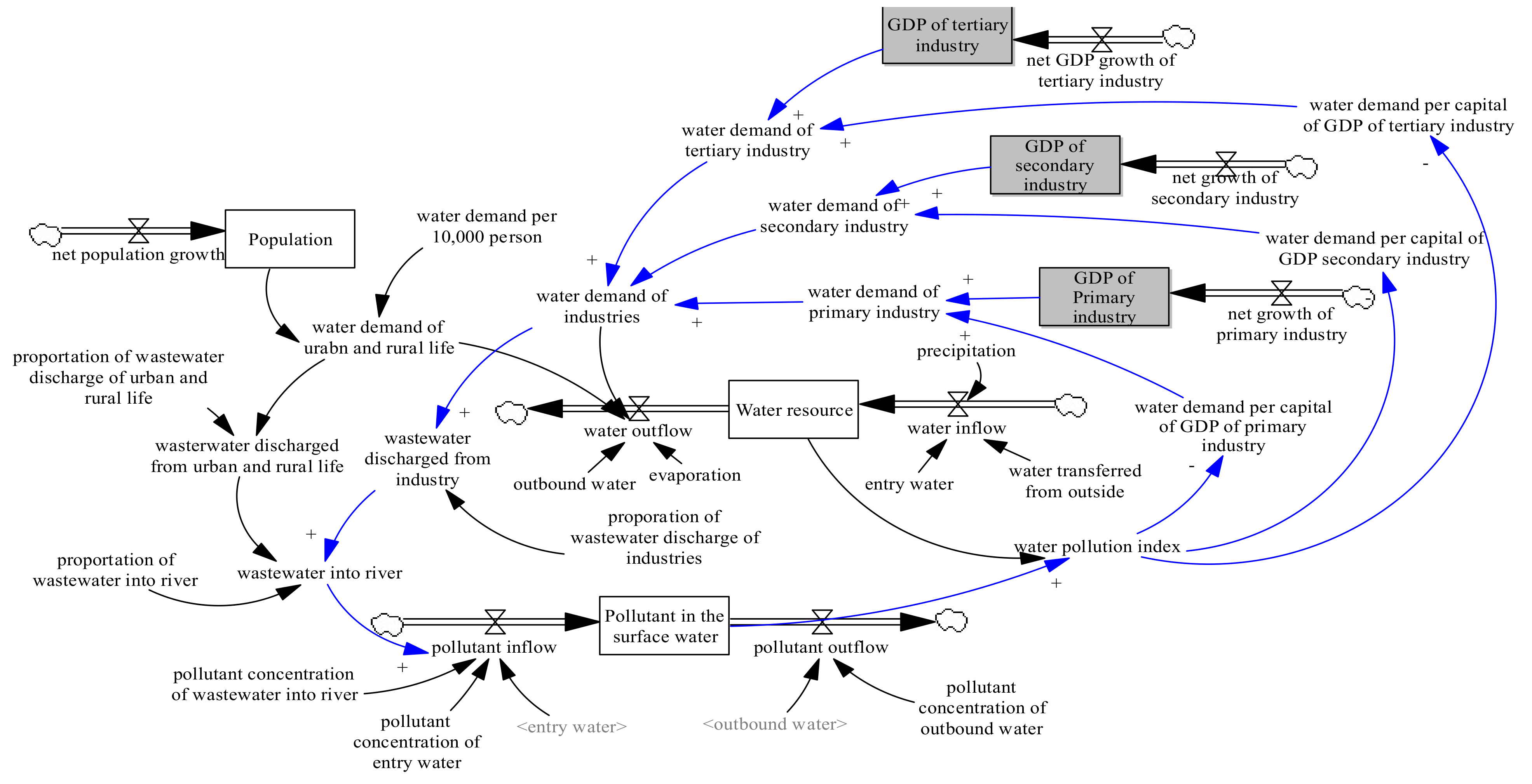
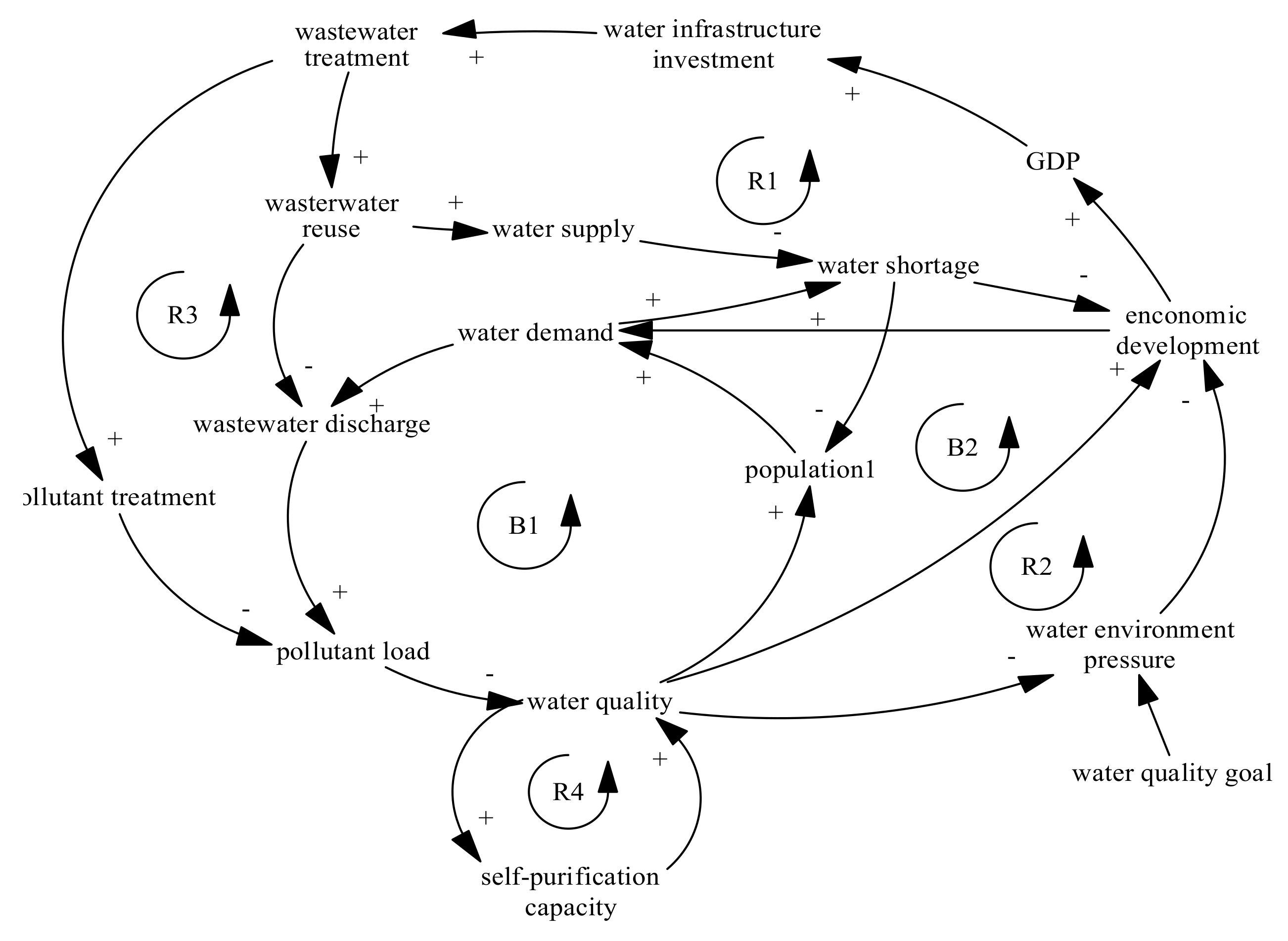
4.2. System Structure of Water Quality

After determining the scope and boundary of the model, the interactions between the four main boundaries of population, economic activities, water supply and demand, and water environment were analyzed. We established a causal-loop diagram for water quality, as shown in Figure 3. The main causal loops in the model causal-loop diagram were based on the following logic:
(1)
The increase of population will increase the water demand, which will have a positive effect on wastewater discharge. More wastewater discharged will bring more pollutant into rivers and lead to the decline of water quality. The deterioration of the water quality has a negative effect on the increase of population.
Loop B1: population → +water demand → +wastewater discharge → +pollutant load → –water quality → +population (balancing loop)
(2)
The development of economy will increase the water demand, which will have a positive effect on wastewater discharge. More wastewater discharged will bring more pollutant into rivers and lead to the decline of water quality. The deterioration of the water quality has a negative effect on the growth of the economy.
Loop B2: economic development → +water demand → +wastewater discharge → +pollutant load → –water quality→ +economic development (balancing loop)
(3)
The growth of the economy will lead to an increase in the local GDP, and the increase in local GDP will increase the investment in water infrastructure. This will positively affect the amount of wastewater treated. More wastewater treatment will contribute to amount of water that can be reused. More water reused will positively affect the water supply. Therefore, the gap between water supply and demand will decrease. The reduction of water shortage will promote economic development.
Loop R1: economic development → +GDP → +water infrastructure investment → +wastewater treatment → +wastewater reuse → +water supply→ –water shortage → –economic development (reinforcing loop)
(4)
The growth of the economy will lead to an increase in the local GDP, and the increase in local GDP will increase the investment in water infrastructure. This will positively affect the amount of wastewater treated. More wastewater treatment will contribute to the amount of water that can be reused, which means the wastewater discharged into the river will decrease. Therefore, the pollutant load will decrease and water quality will improve. High water quality adversely affects water-environment pressure. Less water-environment pressure will positively affect the economic development.
Loop R2: economic development → +GDP→ +water infrastructure investment → +wastewater treatment → +wastewater reuse→ –wastewater discharge → +pollutant load → –water quality → –water environment pressure→ –economic development (reinforcing loop)
(5)
The growth of the economy will lead to an increase in the local GDP, and the increase in local GDP will increase the investment of water infrastructure. This will positively affect the amount of wastewater treated. More wastewater treatment will reduce the pollutant content in wastewater, which means the pollutant load discharged for the river will decrease. Therefore, water quality will increase and water-environment pressure will decrease. Less water-environment pressure will positively affect the economic development.
Loop R3: economic development → +GDP → +water infrastructure investment → +wastewater treatment → +pollutant treatment → –pollutant load → –water quality → –water environment pressure → –economic development (reinforcing loop)
(6)
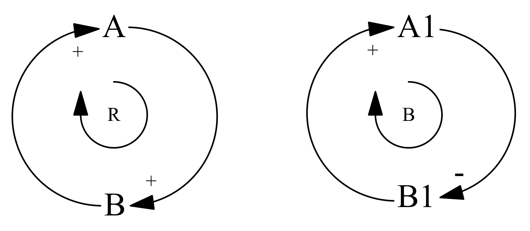
The higher the water quality, the higher the self-purification capacity of a water body.
Loop R4: water quality → +self-purification capacity → +water quality (reinforcing loop)

4.3. Stock-and-Flow Diagram of Water Quality

A stock-and-flow model was developed using Vensim software (Ventana System, Inc., Harvard, MA, USA). The model aimed to assist in the understanding of the coupling of economy and environment. Figure 4 illustrates the key variables of the proposed model, which have been organized in three main sets: the socioeconomic activities (e.g., population; added value of primary, secondary, and tertiary industries), water supply and demand (e.g., water demand of urban and rural life; water demand of primary, secondary and tertiary industries), and the effects of socioeconomic activities on water quality (e.g., the pollutant load of COD, TN, TP, and NH3-N).

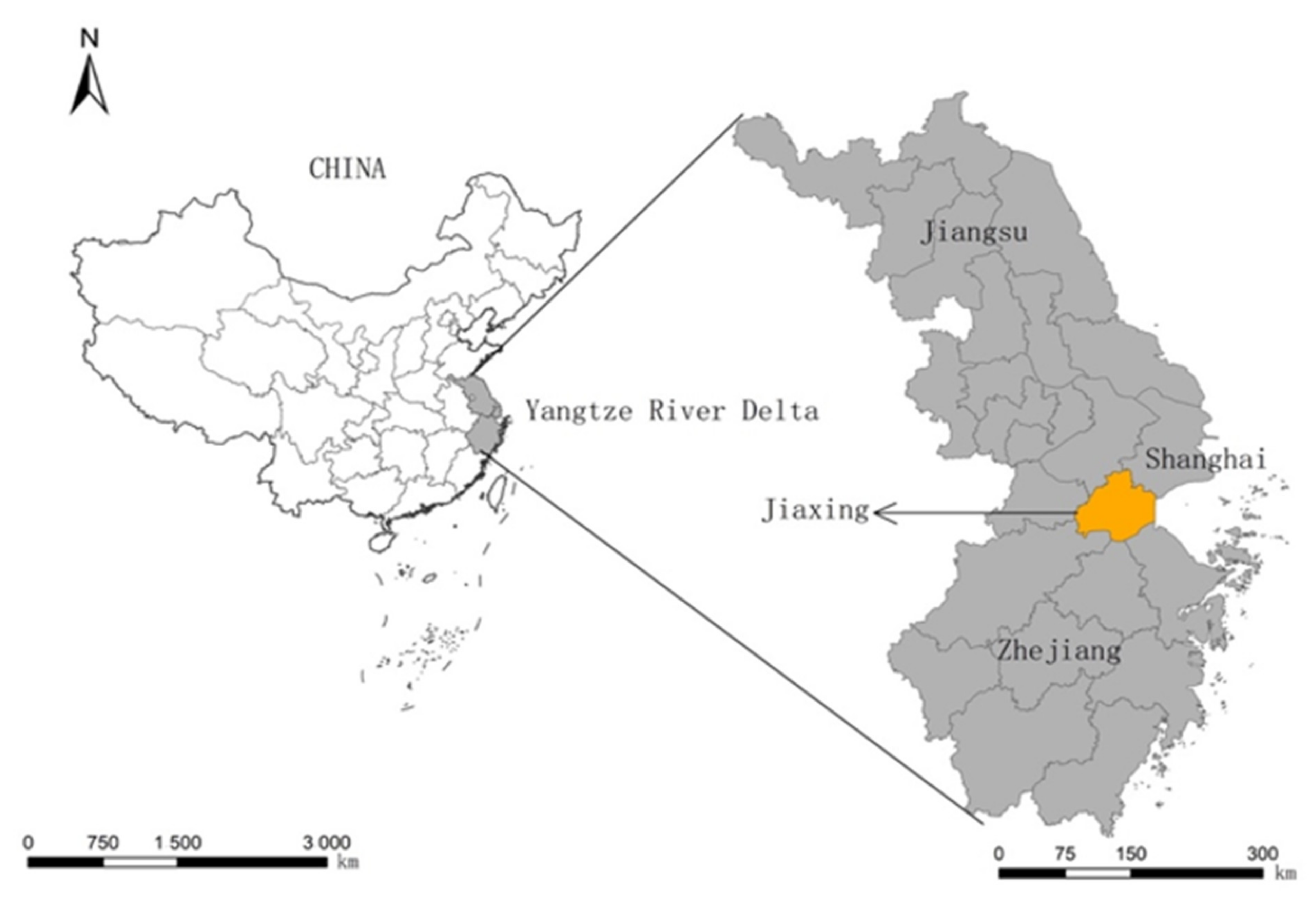
5. Model Adaption to Jiaxing Water Quality

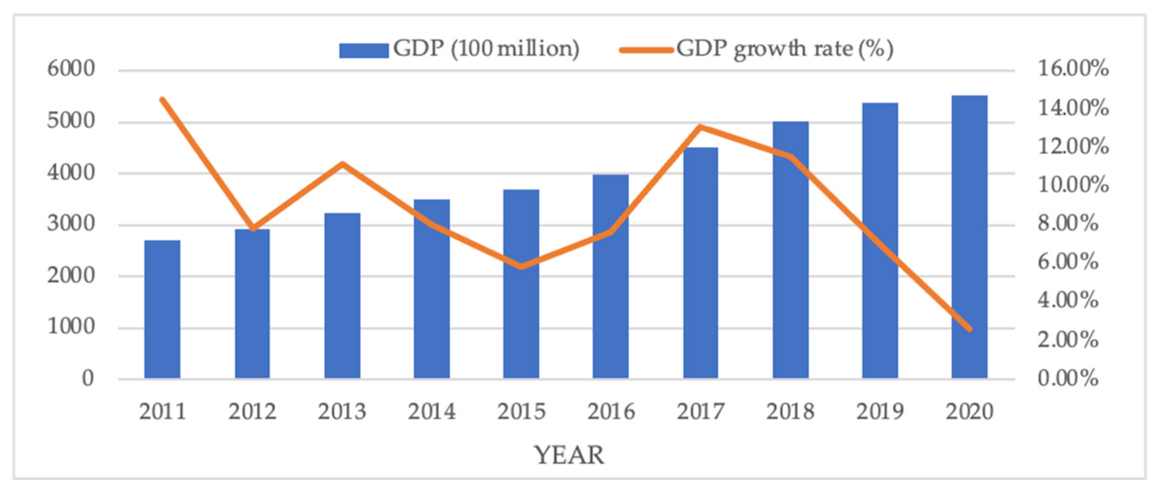
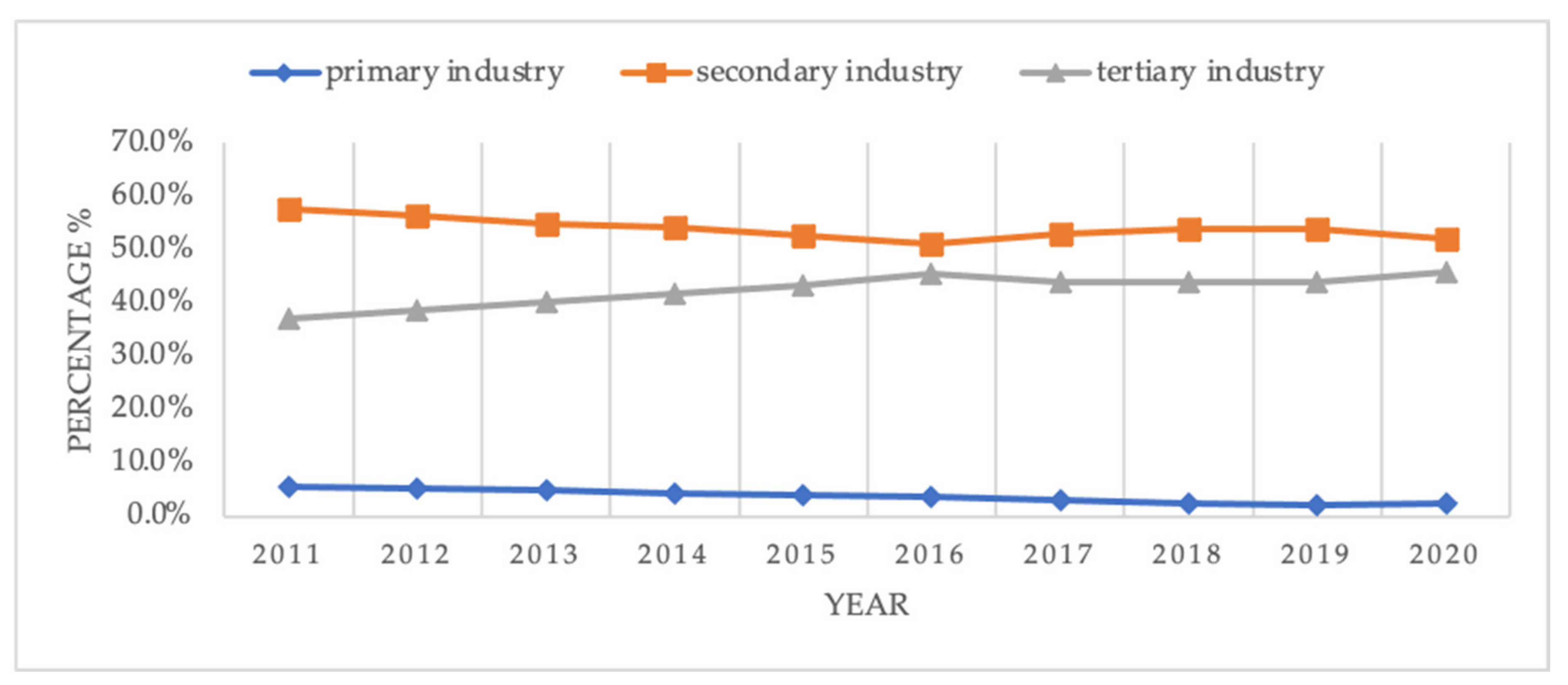
5.1. Overview of the Study Area

Jiaxing is located in the northern part of Zhejiang Province, eastern China. Jiaxing is in the center of the economically dynamic Yangtze River Delta region, and is situated on the railway between Hangzhou and Shanghai. It is joined to the dense waterway network that serves the northern Zhejiang plain (Figure 5). The location is at longitude 120.8106° E and latitude 30.7539° N. It covers an area of 4230.05 km2.
Jiaxing’s economy developed rapidly in the past 10 years (Figure 6). In 2020, the total population of Jiaxing was 4.8 million, and the GDP was RMB 550.95 billion (USD 84.46 billion). Jiaxing’s economic activities are broadly categorized into three sectors: primary, secondary, and tertiary industries. As shown in Figure 7, the primary industry’s contribution to GDP was estimated as 2.3%, with the secondary and tertiary industries accounting for 51.9% and 45.8%, respectively, in 2020 (per the 2021 Jiaxing national economic and social development statistical bulletin).
Jiaxing City is located in the lower reaches of Taihu Lake Basin, which is a typical plain river network area. There are many rivers and lakes in the area. The total length of the rivers is 13,805 km, and the water area is 273.24 km2. Among them, there are 57 main rivers with a total length of 959 km, and 66 lakes with an area of more than 10,000 m2. The total water area is 38.29 km2, with a water area ratio of 7.96%, and a river density of 3.5 km/km2. Since the end of the 20th century, the economy of Jiaxing has developed rapidly, and the five counties (cities) under its jurisdiction have entered the ranks of the top 100 counties in the country. However, the quality of surface water has obviously deteriorated. On the one hand, because it is located at the end of Taihu Lake Basin, it is obviously affected by the water quality. On the other hand, it is also affected by the endogenous pollution brought by economic development, and the surface water quality is deteriorating. Since the end of the 20th century, due to the economic development, the surface water quality of Jiaxing has deteriorated year by year [36], and the main water bodies in the region are inferior to grade V in 2010. Since the 12th Five Year Plan, with the implementation of pollution reduction and other measures, the deterioration trend has been curbed, and the surface water environment is slowly improving. At the end of 2020, the city’s total water resources were 4.217 billion m3, and the annual average precipitation depth was 1640.7 mm (equivalent to 6.929 billion m3 of precipitation). Among the 73 city-controlled sections, a water quality of grade III and above accounted for 91.8%, an increase of 26.0% from the previous year. A water quality of grade IV accounted for 6.8%, and the water quality of grade V accounted for 1.4% (Figure 8). In general, during the 13th Five Year Plan period, the water-environment quality of Jiaxing City has been improved significantly, and the comprehensive improvement effect is remarkable. However, the water quality is still not meeting its expected standard. Further efforts to improve the water quality will be more difficult. This challenge is representative in many ways of other Chinese cities.

5.2. Detailed Setting of the Jiaxing Model

5.2.1. Construction of the Jiaxing Model

The spatial boundary of the Jiaxing SD model was the total administrative area of Jiaxing City. The focus of the water quality was on surface water resources, with particular focus on the impact of sensitive industries on water quality. Sensitive industries are the industries that present the greatest threat to water-quality safety due to industrial development in the region. In this research, we selected the sensitive industries according to the amount of wastewater discharged. Table 2 shows the list of sensitive industries and the proportion of sewage discharged in each industry. Among them, when choosing sensitive industries in primary industry, there was lack of data on the amount of wastewater discharged. Therefore, we considered three subindustries based on available data for the pollutant discharge instead. Since mariculture has less impact on the surface water, our model focused on freshwater aquaculture.
There were a total of 402 variables or constants, including 24 status variables, 32 rate variables, 202 auxiliary variables, 142 constants, and 23 table functions, in the Jiaxing SD model. With the year 2018 as the base year, the data from 2018 to 2020 were used to test the authenticity of the system, and then to forecast the data for 2021–2035. The data sources included: the 2018–2020 Jiaxing Water Resources Bulletin, the Jiaxing City Statistical Yearbook, the Jiaxing City National Economic and Social Development Statistical Bulletin, and the Zhejiang Province Water Resources Yearbook.

5.2.2. Main System Equations

The key equations in the flow diagram of the system dynamics model are listed as follows:
(1)
Pollutant load of COD into the river = pollutant load of COD from urban and rural life + pollutant load of COD from primary industry + pollutant load of COD from secondar industry + pollutant load of COD from tertiary industry
(2)
Pollutant load of COD from primary industry = pollutant load of COD from farming + pollutant load of COD from livestock and poultry + pollutant load of COD from aquaculture
(3)
Pollutant load of COD from farming = wastewater discharged from farming into the river × COD concentration of wastewater discharged from farming
(4)
Wastewater discharged from farming into the river = wastewater discharged from farming × (1 – ecological interception rate of irrigation tail water in farming)
(5)
Wastewater discharged from farming = water demand of farming × proportion of wastewater discharged from farming
(6)
Water demand of farming = GDP of farming × water consumption per capita GDP of farming
(7)
GDP of farming = farming area × average output value per unit area of farming
(8)
Farming area = INTEG (growth rate of farming area – declining rate of farming area, initial value)
To evaluate water quality, we used water quality comprehensive pollution index (WQCPI) evaluation method in this research. The WQCPI is an important method for water-environment assessment, as it can fully depict general water quality [37]. It is calculated based on the evaluation of individual pollution and comprehensive indices. The calculation method for a single pollution index is shown as follows:
P i = C i / S i
where Ci is the measured concentration of the contaminant, and Si is the standard value of the corresponding category. The pollutants measured in this research included COD (chemical oxygen demand), TN (total nitrogen), TP (total phosphorus), and NH3-N (ammoniacal nitrogen).
The calculation method of the water quality comprehensive pollution index is as follows:
P = 1 n i = 1 n P i
The average values determined for P were evaluated to assess the water quality of the surface water (Table 3).

5.3. Model Validation and Sensitivity Analysis

5.3.1. Model Validation

Models do not correspond exactly to the real world because no single model can account for all the factors in a real system [38]. Therefore, SD modelers are more interested in general dynamic tendencies than forecasting specific values of system variables at specific times. Even if the models will never be entirely representative of reality, they can be useful if the models are close enough. Confidence in SD models can be validated by many tests of model structure and behavior. The former test can be compared directly to descriptive knowledge of real-system structure, while the latter one can be conducted by comparing the simulation results with actual data [39].
Both the structure and behavior test were performed in this research. We first conducted a structure-verification test in terms of dimensional consistency. The unit check tool of Vensim was used, and there was no dimensional mismatch. Then, in the process of the behavior test, the simulated result was compared with the relevant historical data of Jiaxing City in 2018–2020. The comparison of historical and simulated data of the resident population and GDP of three industries in Jiaxing City is given in Table 4, while the comparison of water usage is shown in Table 5.
Table 4 and Table 5 demonstrate that the error rate between all simulated data and real data was below 10%, which means the model was in line with the actual situation and can be considered to be adequate to forecast further time steps [40]. Therefore, the developed model could be used to analyze and forecast the dynamic change of water quality in the next step.

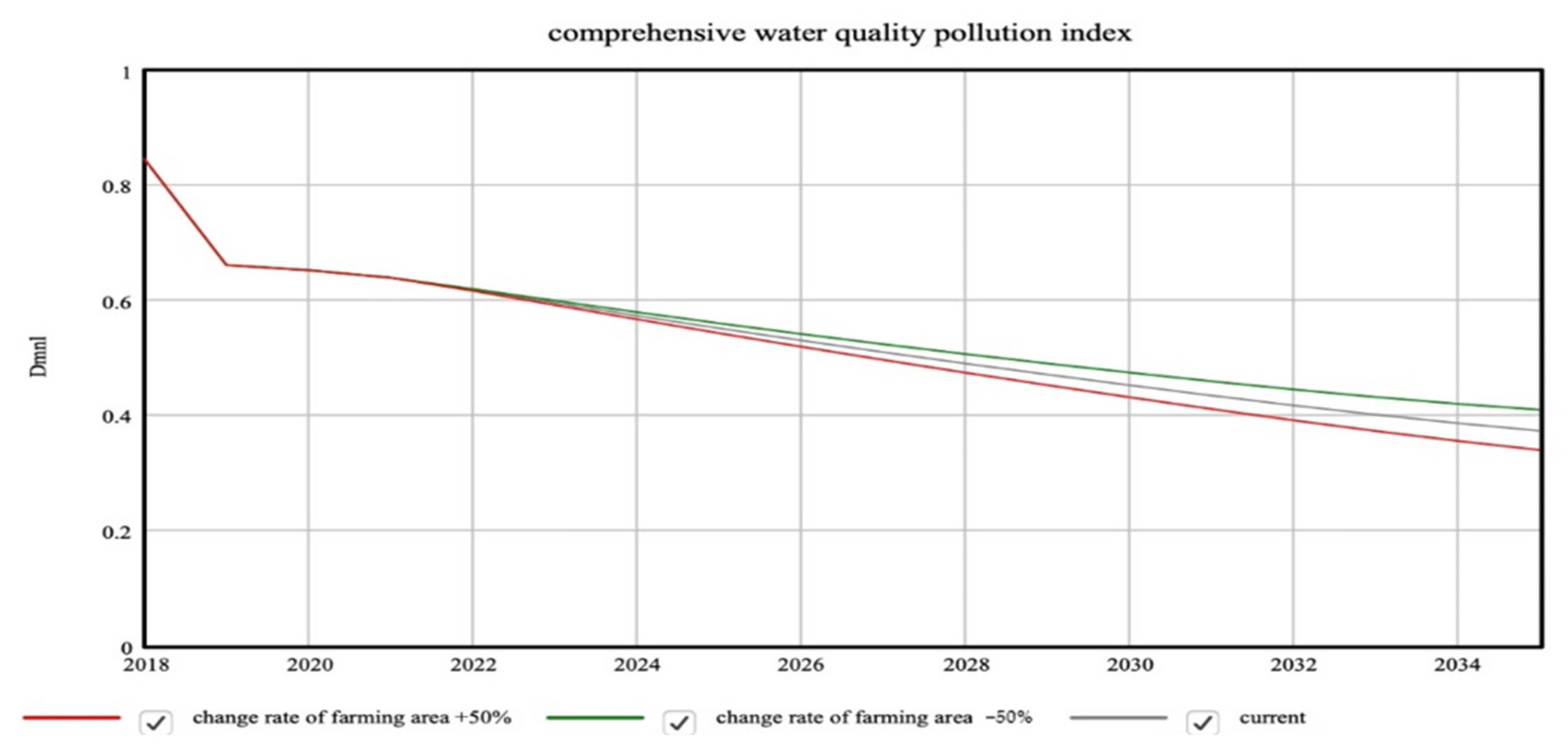
5.3.2. Sensitivity Analysis

Sensitivity analysis is an important task for the reliability of simulation results due to the uncertainties embedded in parameters of SD models. This analysis can be used to ascertain model response to uncertain changing of industrial-structure adjustment and identify influential parameters affecting water quality. We selected nine parameters related to the change in industry proportion for carrying out a sensitivity analysis of the complex system: three parameters that were associated with primary industry (change rate of farming area, change rate of LPB GDP, change rate of aquaculture GDP), three that were related to the secondary industry (change rate of TI added value, change rate of PPP added value, change rate of RCMCP added value), and three related to the tertiary industry (change rate of WRS added value, change rate of ACS added value, change rate of CSE added value). Figure 9 gives the sensitivity analysis of “the change rate of farming area” as an example. The sensitivity analysis indicated that the curves obtained were consistent with the original trends.
Table 6 gives the deviation trends of five water-quality variables (COD concentration, NH3-N concentration, TN concentration, TP concentration, and WQCPI) obtained by adjusting the initial value of these nine parameters selected 50% up or down. The deviation in 2035 was larger than that in 2025, which suggests that the present model was robust enough to simulate the coupling mechanism of economic development and water environment. The sensitivity analysis results also showed that adjustment in farming industry had the most significant impact on water quality, followed by PPP and LPB. In the perspective of single pollutant concentration, the concentration of COD and TN was much more sensitive to the change of the farming industry, while PPP and LPB were identified as the most sensitive indicators of the concentrations of NH3-N and TP, respectively.

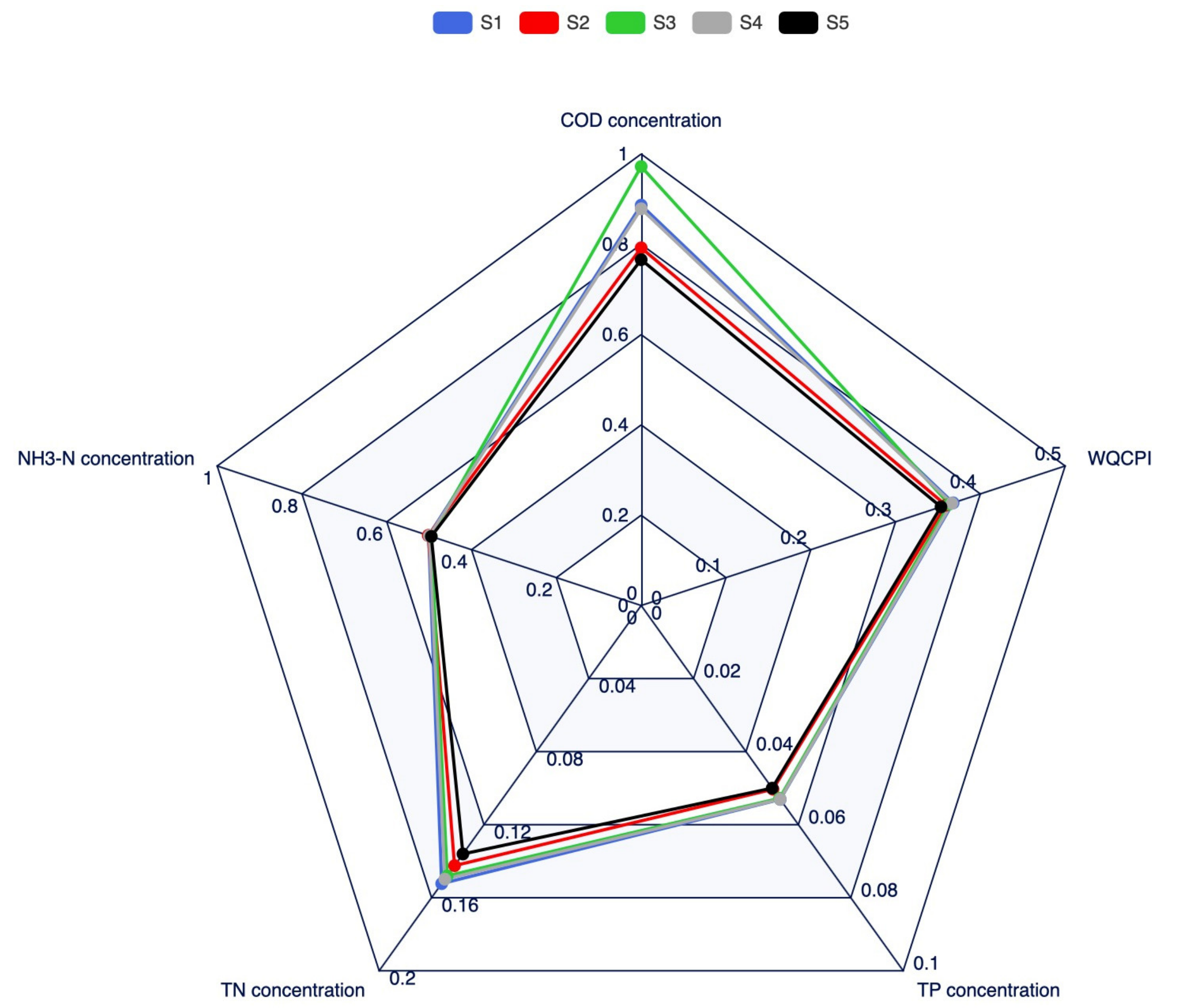
5.4. Model Simulation and Analysis

On the basis of constructing the composite system simulation model and verifying its effectiveness, this research tested the dynamic impact of water environment by setting scenario assumptions for different degrees of industrial-structure adjustment. Among them, the adjustment of industrial structure should be realized by changing the different industries’ growth rate. According to the 14th Five Year Plan and the related industrial development plan of Jiaxing, the scenarios are as follows:
Scenario 1 (development as usual): there was no parameter adjustment in this scenario. The scenario was used as a reference scenario; that is, to maintain the existing level of industrial-structure development, and the growth rate of the GDP of the primary, secondary, and tertiary industries remained constant.
Scenario 2 (structural optimization of primary industry): this scenario gave priority to adjustment in the distribution of primary industry. Nonpoint source pollution caused by irrigation and family livestock and poultry breeding plays a major role in the deterioration of water quality in Jiaxing City. Livestock and poultry breeding was an important pillar industry in Jiaxing during the early 20th century. Large-scale livestock and poultry breeding with the phenomenon of direct discharge of livestock manure into rivers exceeded the water-environment carrying capacity. Meanwhile, the scale of aquaculture was expanding due to the promotion of green technology. Therefore, in 2013, Jiaxing government started checking and rectifying illegal breeding farms and achieved demonstrated results. In Scenario 2, a 10% decrease in the change rate of farming area and livestock and poultry breeding GDP and a 10% increase in the change rate of aquaculture GDP were applied after 2021.
Scenario 3 (structural optimization of secondary industry): this scenario focused on adjustment of the distribution of the secondary industry. Considering the textile industry, paper and paper product production industry, and raw chemical materials and chemical products industries are intensive industries for the consumption of water and discharge highly polluted water in large amounts, Jiaxing City will take actions to limit the growth of these industries. Thus, Scenario 3 assumed the current change rate of these industries will decline 10% from 2021.
Scenario 4 (structural optimization of tertiary industry): this scenario devoted attention to adjustment of the distribution of the tertiary industry. During the 13th Five Year Plan period, the proportion of added value of the information service industry, financial industry, science and technology service industry, and other modern service industries in Jiaxing City has been increasing. There will be a slowdown in the development of traditional service industries as more resources are transferred to the modern service industries. In this scenario, the change rates of WRS added value, ACS added value, and CSE added value will have a decrease of 10% from 2021.
Scenario 5 (collaborative optimization of three industries): this scenario was a coordinated adjustment of the distribution of the three industries. This integration scenarios took all the parameter adjustments into consideration.
As this research aimed to explore the impact of industrial-structure adjustment on water quality, the scenario design did not consider the optimization of economic objectives. Table 7 gives an introduction to the parameter settings in different scenarios.

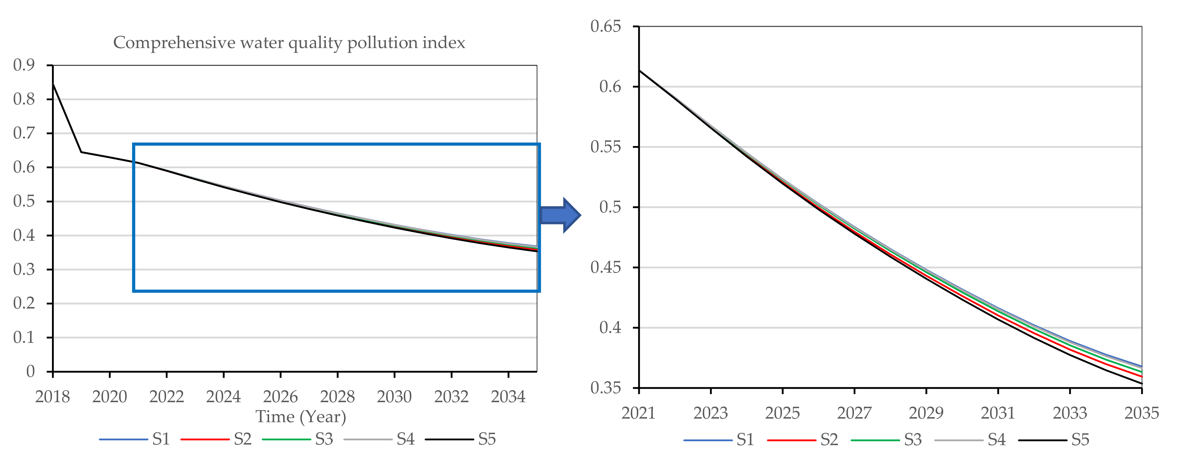
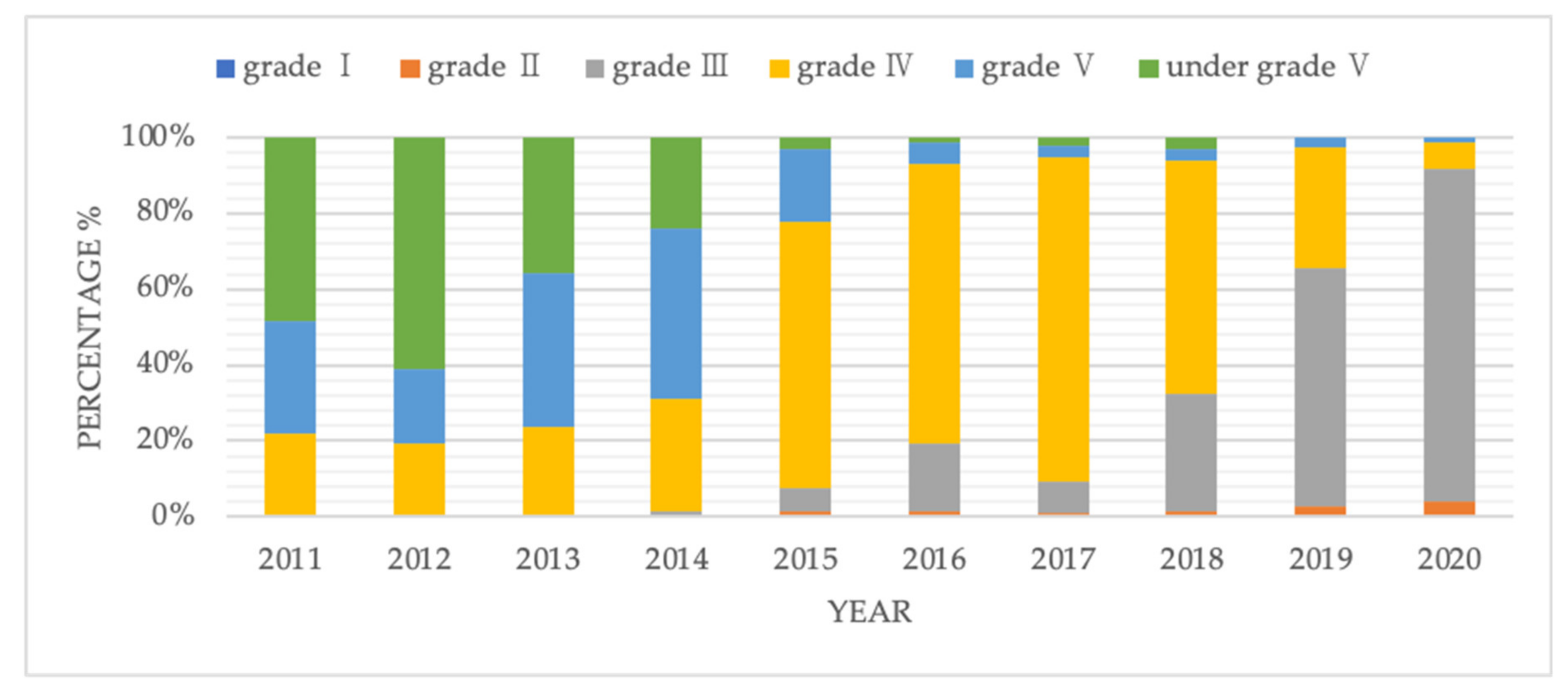
5.4.1. Simulation of Water Quality

The simulated WQCPI of surface water in Jiaxing City is shown in Figure 10. Under the current industrial structure and economic development mode, the quality of the surface-water environment in Jiaxing City will be significantly improved and achieve a subcleanness level. Specifically, the comprehensive pollution index of the surface-water environment decreased rapidly from 2021 to 2030, and decreased slowly from 2031 to 2035. By 2035, the comprehensive pollution index of water environment will drop to about 0.37, with COD, NH3-N, TN, and TP concentrations in Jiaxing’s surface water of 0.89, 0.5, 0.15, and 0.05 mg/L, respectively. Compared with the base mode, the other four alternative scenarios pushed the CWQPI curve downward at different levels, which meant the adjustments of industrial structure could promote the improvement of water quality, especially in reducing COD concentration (Figure 11). Among the four policy designs of industrial-structure optimization, collaborative optimization of three industries (S5) was the most effective in improving water quality, indicating that transformation and upgrading of the three industrial structures would be the most beneficial and most efficient measure to promote sustained development of Jiaxing City’s water environment. However, the simulation results also indicated that this effect was limited, and cannot help Jiaxing’s water quality achieve breakthrough.

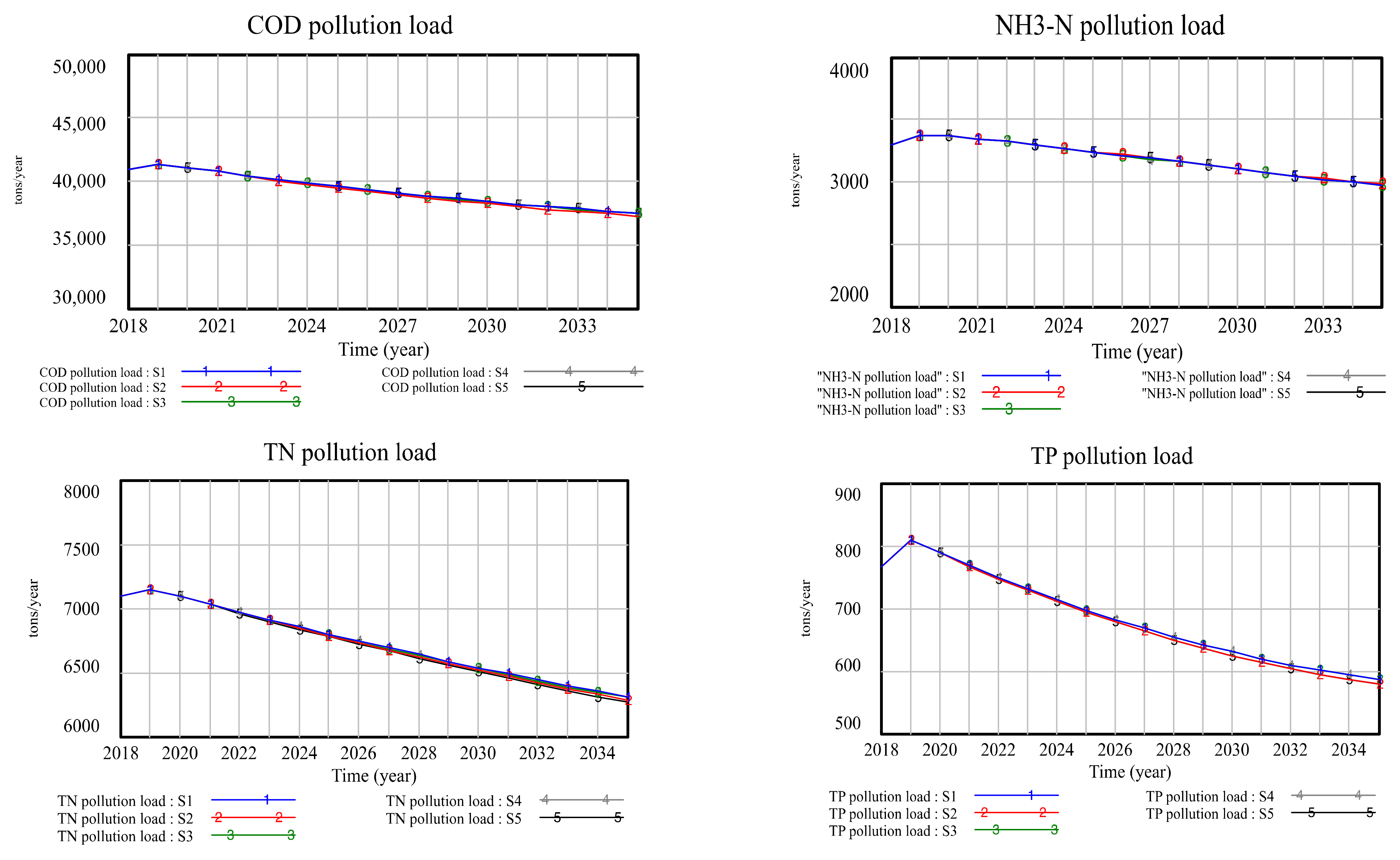
5.4.2. Simulation of Pollution Load

Figure 12 gives the simulation results for COD, NH3-N, TN, and TP pollution loads from socioeconomic activities between 2018 and 2035 under different scenarios. Four pollutant-loading trends behaved in the same way. Pollutant discharged from socioeconomic activities will gradually decrease after a temporary increase in 2019. Taken as a whole, industrial-structure adjustments had positive effects on reducing pollutant load. They can especially contribute to the reduction of COD and TP discharges.

5.5. Suggestions for Improving Water Quality of Jiaxing

This research sought to develop sustainable solutions for water-quality management by conducting scenario analyses. The results of the sensitivity analysis showed that adjustment in the farming industry had the most significant impact on WQCPI, followed by PPP and LPB, which indicated that these three industries are critical components that affect Jiaxing City’s water-quality management. This is reasonable, because agricultural nonpoint sources of pollution are the leading source for the surface water environment. The simulation results indicated that the existing industrial structure of Jiaxing City will improve the water quality during 14th Five Year Plan period. However, the adjustment of industrial structure in Jiaxing City has little influence on water-quality improvement at the present stage. On the one hand, the Jiaxing government had implemented strict measures to control and prevent industrial pollution, and some of the most persistent point-source pollutants are under good control now. On the other hand, there is little space for the major industries to adjust, as they have long been competitive industries in Jiaxing. Therefore, to ensure the sustainability of water quality, the Jiaxing government should take actions to accelerate the application of cleaner production processes and technologies into consideration. It is necessary to increase investment support for cleaner production transformation projects of key industries and enterprises in the river basin and organize cleaner production pilot demonstrations. For example, enterprises should give priority to the cleaner production technology issued by the state.
The results of the SD models can be used to investigate the interactions among numerous factors and understand the dynamic behavior of complex systems. However, the social economy and water environment constitute an open and dynamic system with the characteristics of high complexity, uncertainty, and multiple levels. While making model-based assessments of complex environmental problems, the assessments should rely more on exploring possible future developments, rather than making accurate predictions about the future [41]. The impact of possible future policies can be analyzed by conducting scenario analyses and providing reference for decision-makers. For example, the results of Scenario 5 showed that the impact of industrial-structure adjustment on NH3-N pollutant load was very limited, which indicated that industrial-structure adjustment is not an effective way to degrade the concentration of NH3-N in surface water.
This research had limitations. First, some variables, such as the amount of entry water, outland water, precipitation, and evaporation, were assumed to be constant. This implies that the gap between water supply and demand cannot be measured precisely. Second, the impact of water quality on economic activities was simplified by industrial water quota, as it was quite difficult to quantify the interaction between water quality and the economic change of each sensitive industries. Third, a multiobjective optimization study of economic growth and water-quality improvement was not considered. Future research is required to make up for these deficiencies.

6. Conclusions

This research used SD modelling as a decision-support tool to help achieve sustainable water-quality management. The model used in this work covered population; primary, secondary, and tertiary industries; water resources; and water environmental subsystems. Sectors of population and economics, water demand and wastewater discharge, pollutant load, and water quality were coupled in the SD model in order to express the coupling coordination among the city’s socioeconomic development, pollutant loads, and water quality.
We applied the model to Jiaxing City and the primary, secondary, and tertiary industries were further divided into nine subindustries. The model was calibrated based on the historical data obtained from 2018–2020. Validation results and sensitivity analysis confirmed the model was appropriately implemented and could be used to analyze the research problem. Under the current scenario (S1), Jiaxing’s water quality will steadily improve over the period of 2021–2035 and reach a subcleanness level at the end of 14th Five Year Plan. Adjustments in the farming industry had the most significant impact on water quality, followed by PPP and LPB. In terms of individual pollutants, the concentrations of COD and TN were much more sensitive to changes in the farming industry than in other industries. PPP and LPB were identified as having the most influence on the concentrations of NH3-N and TP, respectively. Collaborative optimization of the three industries (S5) would be the most efficient policy to promote sustainable water management. However, the effect of industrial-structure adjustment was limited. Strategies comprising cleaner production should be undertaken to reduce pollution generation.

Author Contributions

L.W. proposed the research design, developed the model, conducted model validation, and wrote the paper; H.Y. participated in the research design and model development, and revised the manuscript; R.W. guided the research process and revised the manuscript. All authors have read and approved the final manuscript.

Funding

This research was supported by the National Science and Technology Major Project of China on Water Pollution Control and Management (2017ZX07206-001).

Data Availability Statement

The data presented in this study are available upon request from the corresponding author.

Acknowledgments

The authors give thanks to the Jiaxing Water-Affair Authority for operational data. The authors are also very grateful for the comments from the editor and the anonymous reviewers.

Conflicts of Interest

The authors declare no conflict of interest. The funding supports did not influence the analyses conducted or the conclusions reached in this study.

References

  1. Gu, X.; Liao, Z.; Zhang, G.; Xie, J.; Zhang, J. Modelling the effects of water diversion and combined sewer overflow on urban inland river quality. Environ. Sci. Pollut. Res. 2017, 24, 21038–21049. [Google Scholar] [CrossRef]
  2. Yang, W.; Li, L. Efficiency evaluation and policy analysis of industrial wastewater control in China. Energies 2017, 10, 1201. [Google Scholar] [CrossRef]
  3. Yang, N.; Zhang, Z.; Xue, B.; Ma, J.; Chen, X.; Lu, C. Economic Growth and Pollution Emission in China: Structural Path Analysis. Sustainability 2018, 10, 2569. [Google Scholar] [CrossRef] [Green Version]
  4. Li, T.; Yang, S.; Tan, M. Simulation and optimization of water supply and demand balance in Shenzhen: A system dynamics approach. J. Clean. Prod. 2019, 207, 882–893. [Google Scholar] [CrossRef]
  5. Naderi, M.M.; Mirchi, A.; Bavani, A.R.M.; Goharian, E.; Madani, K. System dynamics simulation of regional water supply and demand using a food-energy-water nexus approach: Application to Qazvin Plain, Iran. J. Environ. Manag. 2021, 280, 111843. [Google Scholar] [CrossRef] [PubMed]
  6. Li, K.; Ma, T.; Wei, G.; Zhang, Y.; Feng, X. Urban Industrial Water Supply and Demand: System Dynamic Model and Simulation Based on Cobb–Douglas Function. Sustainability 2019, 11, 5893. [Google Scholar] [CrossRef] [Green Version]
  7. Ma, W.; Meng, L.; Wei, F.; Opp, C.; Yang, D. Sensitive Factors Identification and Scenario Simulation of Water Demand in the Arid Agricultural Area Based on the Socio-Economic-Environment Nexus. Sustainability 2020, 12, 3996. [Google Scholar] [CrossRef]
  8. Wang, X.; Zhang, J.; Shamsuddin, S.; He, R.; Xia, X.; Mou, X. Potential impact of climate change on future water demand in Yulin city, Northwest China. Mitig. Adapt. Strateg. Glob. Chang. 2015, 20, 1–19. [Google Scholar]
  9. Liu, H.; Benoit, G.; Liu, T.; Liu, Y.; Guo, H. An integrated system dynamics model developed for managing lake water quality at the watershed scale. J. Environ. Manag. 2015, 155, 11–23. [Google Scholar] [CrossRef]
  10. Zeilhofer, P.; Lima, E.B.N.R.; Lima, G.A.R. Land use effects on water quality in the urban agglomeration of Cuiabá and Várzea Grande, Mato Grosso State, central Brazil. Urban Water J. 2010, 7, 173–186. [Google Scholar] [CrossRef]
  11. Juma, D.W.; Wang, H.; Li, F. Impacts of population growth and economic development on water quality of a lake: Case study of Lake Victoria Kenya water. Environ. Sci. Pollut. Res. 2014, 21, 5737–5746. [Google Scholar] [CrossRef] [PubMed]
  12. Liu, Y.; Engel, B.A.; Flanagan, D.C.; Gitau, M.W.; McMillan, S.K.; Chaubey, I. A review on effectiveness of best management practices in improving hydrology and water quality: Needs and opportunities. Sci. Total Environ. 2017, 601, 580–593. [Google Scholar] [CrossRef] [PubMed]
  13. Whitehead, P.G.; Wilby, R.L.; Battarbee, R.W.; Kernan, M.; Wade, A.J. A review of the potential impacts of climate change on surface water quality. Hydrol. Sci. J. 2009, 54, 101–123. [Google Scholar] [CrossRef]
  14. Dhote, S.; Dixit, S. Water quality improvement through macrophytes—A review. Environ. Monit. Assess. 2009, 152, 149–153. [Google Scholar] [CrossRef]
  15. Chen, Z.; Wei, S. Application of system dynamics to water security research. Water Resour. Manag. 2014, 28, 287–300. [Google Scholar] [CrossRef]
  16. Karamouz, M.; Akhbari, M.; Moridi, A.; Kerachian, R. A system dynamics-based conflict resolution model for river water quality management. Iran. J. Environ. Health Sci. Eng. 2006, 3, 147–160. [Google Scholar]
  17. Duran-Encalada, J.A.; Paucar-Caceres, A.; Bandala, E.R.; Wright, G.H. The impact of global climate change on water quantity and quality: A system dynamics approach to the US–Mexican transborder region. Eur. J. Oper. Res. 2017, 256, 567–581. [Google Scholar] [CrossRef] [Green Version]
  18. Nozari, H.; Liaghat, A. Simulation of drainage water quantity and quality using system dynamics. J. Irrig. Drain. Eng. 2014, 140, 05014007. [Google Scholar] [CrossRef]
  19. Park, S.; Kim, B.J.; Jung, S.Y. Simulation methods of a system dynamics model for efficient operations and planning of capacity expansion of activated-sludge wastewater treatment plants. Procedia Eng. 2014, 70, 1289–1295. [Google Scholar] [CrossRef] [Green Version]
  20. Wang, G.; Wang, S.; Kang, Q.; Duan, H.; Wang, X.E. An integrated model for simulating and diagnosing the water quality based on the system dynamics and Bayesian network. Water Sci. Technol. 2016, 74, 2639–2655. [Google Scholar] [CrossRef]
  21. Debele, B.; Srinivasan, R.; Parlange, J.Y. Coupling upland watershed and downstream waterbody hydrodynamic and water quality models (SWAT and CE-QUAL-W2) for better water resources management in complex river basins. Environ. Model. Assess. 2008, 13, 135–153. [Google Scholar] [CrossRef]
  22. Li, K.; He, J.; Li, J.; Guo, Q.; Liang, S.; Li, Y.; Wang, X. Linking water quality with the total pollutant load control management for nitrogen in Jiaozhou Bay, China. Ecol. Indic. 2018, 85, 57–66. [Google Scholar] [CrossRef]
  23. Forrester, J.W. Industrial Dynamics; MIT Press: Cambridge, MA, USA, 1961. [Google Scholar]
  24. Doyle, J.C.; Francis, B.A.; Tannenbaum, A.R. Feedback Control Theory; Courier Corporation: North Chelmsford, MA, USA, 2013. [Google Scholar]
  25. Richmond, B. Systems thinking: Critical thinking skills for the 1990s and beyond. Syst. Dynam. Rev. 1993, 9, 113–133. [Google Scholar] [CrossRef] [Green Version]
  26. Barlas, Y. System dynamics: Systemic feedback modeling for policy analysis. System 2007, 1, 1–29. [Google Scholar]
  27. Senge, P.M.; Sterman, J.D. Systems thinking and organizational learning: Acting locally and thinking globally in the organization of the future. Eur. J. Oper. Res. 1992, 59, 137–150. [Google Scholar] [CrossRef]
  28. Sterman, J.D. Business Dynamics: Systems Thinking and Modeling for a Complex World; McGraw-Hill: New York, NY, USA, 2000. [Google Scholar]
  29. Ford, F.A. Modeling the Environment: An Introduction to System Dynamics Models of Environmental Systems; Island Press: Washington, DC, USA, 1999. [Google Scholar]
  30. Mulligan, M.; Wainwright, J. Modelling and model building. In Environmental Modelling: Finding Simplicity in Complexity; John Wiley & Sons: Hoboken, NJ, USA, 2004; pp. 7–73. [Google Scholar]
  31. Yang, C.C.; Chang, L.C.; Ho, C.C. Application of system dynamics with impact analysis to solve the problem of water shortages in Taiwan. Water Resour. Manag. 2008, 22, 1561–1577. [Google Scholar] [CrossRef]
  32. Fang, Y.; Lim, K.; Qian, Y.; Feng, B. System dynamics modeling for information systems research theory development and practical application. MIS Q. 2018, 24, 1303–1329. [Google Scholar]
  33. Zhao, J.; Jia, J.; Qian, Y.; Zhong, L.; Wang, J.; Cai, Y. COVID-19 in Shanghai: IPC policy exploration in support of work resumption through system dynamics modeling. Risk Manag. Healthc. Policy 2020, 13, 1951. [Google Scholar] [CrossRef]
  34. Mirchi, A.; Madani, K.; Watkins, D.; Ahmad, S. Synthesis of system dynamics tools for holistic conceptualization of water resources problems. Water Resour. Manag. 2012, 26, 2421–2442. [Google Scholar] [CrossRef]
  35. Simonovic, S.P. Managing Water Resources: Methods and Tools for a Systems Approach; Routledge: London, UK, 2012. [Google Scholar]
  36. Shao, W. Effectiveness of water protection policy in China: A case study of Jiaxing. Sci. Total Environ. 2010, 408, 690–701. [Google Scholar] [CrossRef]
  37. Tao, T.; Yujia, Z.; Huang, K. Water quality analysis and Recommendations through comprehensive pollution index method. Manag. Sci. Eng. 2011, 5, 95–100. [Google Scholar]
  38. Barisa, A.; Rosa, M. A system dynamics model for CO2 emission mitigation policy design in road transport sector. Energy Procedia 2018, 147, 419–427. [Google Scholar] [CrossRef]
  39. Forrester, J.W.; Senge, P.M. Tests for building confidence in system dynamics models. In TIMS Studies in the Management Science; North Holland Press: Amsterdam, The Netherlands, 1980. [Google Scholar]
  40. Li, K.B.; Ma, T.Y.; Wei, G. Multiple Urban Domestic Water Systems: Method for Simultaneously Stabilized Robust Control Decision. Sustainability 2018, 10, 4092. [Google Scholar] [CrossRef] [Green Version]
  41. Kelly, R.A.; Jakeman, A.J.; Barreteau, O.; Borsuk, M.E.; ElSawah, S.; Hamilton, S.H.; Henriksen, H.J.; Kuikka, S.; Maier, H.R.; Rizzoli, A.E.; et al. Selecting among five common modelling approaches for integrated environmental assessment and management. Environ. Model. Softw. 2013, 47, 159–181. [Google Scholar] [CrossRef]
Figure 1. Feedback loops in system dynamics.
Sustainability 13 07696 g001
Figure 2. Stock-and-flow structure in system dynamics.
Sustainability 13 07696 g002
Figure 3. Causal-loop diagram of water quality.
Sustainability 13 07696 g003
Figure 4. Simplified stock-and-flow diagram of water quality.
Sustainability 13 07696 g004
Figure 5. Location of Jiaxing City.
Sustainability 13 07696 g005
Figure 6. GDP and GDP growth rate of Jiaxing City (source: 2011–2020 Jiaxing national economic and social development statistical bulletins).
Sustainability 13 07696 g006
Figure 7. Value added (% GDP) of the three sectors in Jiaxing City (source: 2011–2020 Jiaxing national economic and social development statistical bulletins).
Sustainability 13 07696 g007
Figure 8. Water quality of surface water in Jiaxing from 2011 to 2020 (source: 2011–2020 Jiaxing water resource bulletins).
Sustainability 13 07696 g008
Figure 9. Sensitivity analysis of WQCPI in response to “the change rate of farming area” ±50%.
Sustainability 13 07696 g009
Figure 10. Simulated WQCPI of surface water in Jiaxing City (2018–2035).
Sustainability 13 07696 g010
Figure 11. Radar chart for the simulation of water quality in 2035 under different scenarios.
Sustainability 13 07696 g011
Figure 12. Simulation of COD, NH3-N, TN, and TP pollution loads from socioeconomic activities between 2018 and 2035 under different scenarios.
Sustainability 13 07696 g012
Table 1. System elements of water/quality.
SubsystemSpecific Key ParametersUnit
Population subsystemUrban population10,000 persons
Rural population10,000 persons
Natural growth rate of urban population1/year
Mechanical growth rate of urban population1/year
Primary industry subsystemFarming area10,000 ha
Growth rate of farming area1/year
Water consumption per RMB 10,000 output value10,000 t/RMB 10,000
Proportion of wastewater generatedDimensionless
Proportion of wastewater discharged into riverDimensionless
Secondary industry subsystemGDPRMB 10,000
Growth rate of GDP 1/year
Water consumption for per RMB 10,000 output value10,000 t/RMB 10,000
Proportion of wastewater generatedDimensionless
Reuse rate of treated wastewaterDimensionless
Proportion of wastewater discharged into riverDimensionless
Tertiary industry subsystemGDPRMB 10,000
Growth rate of GDP1/year
Water consumption for per RMB 10,000 output value10,000 tons/ RMB 10,000
Proportion of wastewater generatedDimensionless
Proportion of wastewater discharged into riverDimensionless
Water resource subsystemWater resources10,000 t
Domestic water consumption10,000 t
Production water consumption10,000 t
Ecological water consumption10,000 t
Precipitation10,000 t
Evaporation10,000 t
Water environment subsystemCOD (chemical oxygen demand) pollutant loadt
NH3-N (ammoniacal nitrogen) pollutant loadt
TN (total nitrogen) pollutant loadt
TP (total phosphorus) pollutant loadt
Table 2. List of sensitive industries.
SectorKey IndustriesProportion of Wastewater Discharged
Primary industryFarming-
Livestock and poultry breeding (LPB) -
(Freshwater) aquaculture-
Secondary industryTextile industry (TI)53.63%
Paper and paper products (PPP) 16.74%
Raw chemical materials and chemical products (RCMCP)8.01%
Tertiary industryWholesale and retail sale (WRS)32.02%
Accommodation and catering services (ACS)22.71%
Culture, sports, and entertainment (CSE)26.36%
Table 3. Grading standard for water-quality classification.
Comprehensive
Pollution Index
LevelClassification Basis
≤0.2CleannessMost of the items were not detected, and some items were detected but within the standard.
0.21~0.40SubcleannessThe detection value was within the standard, and individual items were close to or exceeded the standard.
0.41~0.7Slight pollutionIndividual items were detected and exceeded the standard.
0.71~1.00Moderate pollutionTwo of the detected values exceeded the standard.
1.01~2.0Heavy pollutionA considerable part of the detected values exceeded the standard.
≥2.01Severe pollutionA considerable part of the detected values exceeded the standard several times or dozens of times.
Table 4. Comparison of historical and simulated data of the population (million) and GDP (billion RMB).
Year201820192020
PopulationReal value472.6480540.1
Simulated value472.6480.13540.41
Error rate0%0.03%0.06%
GDP of primary industryReal value195.14201.7-
Simulated value195.14199.01-
Error rate0%1.33%-
Added value of secondary industryReal value2755.692892.552861.09
Simulated value2755.692863.962888.03
Error rate0%1%0.94%
Added value of tertiary industryReal value2146.762356.882524.25
Simulated value2146.762346.142502.64
Error rate0%0.46%0.86%
Table 5. Comparison of historical and simulated data of water use (billion tons).
Year201820192020
Domestic water consumptionReal value2.292.322.41
Simulated value2.292.322.62
Error rate0%0%8.71%
Primary industry water consumptionReal value10.279.629.36
Simulated value10.279.629.45
Error rate0%0%1%
Secondary industry water consumptionReal value4.324.604.53
Simulated value4.324.584.55
Error rate0%0.43%0.44%
Tertiary industry water consumptionReal value1.281.291.35
Simulated value1.281.331.35
Error rate0%3.1%0%
Table 6. Sensitivity analysis of WQCPI in response to nine parameters ±50%.
ParameterCOD Concentration
(mg/L)
NH3-N Concentration
(mg/L)
TN Concentration
(mg/L)
TP Concentration
(mg/L)
WQCPI
2025203520252035202520352025203520252035
Change rate of farming area0.0550.2380.0000.0070.0060.0260.0000.0040.0040.022
Change rate of LPB GDP0.0420.0950.0040.0090.0080.0170.0030.0070.0080.018
Change rate of aquaculture GDP0.0090.0240.0060.0160.0040.0110.0000.0010.0040.011
Change rate of TI added value0.0010.0040.0000.0000.0000.0010.0000.0000.0000.000
Change rate of PPP added value0.0150.0640.0010.0290.0040.0110.0000.0010.0020.020
Change rate of RCMCP added value0.0080.1230.0000.0030.0020.0030.0000.0000.0010.002
Change rate of WRS added value0.0050.0270.0000.0050.0010.0080.0000.0000.0010.004
Change rate of ACS added value0.0000.0040.0000.0020.0000.0010.0000.0000.0000.002
Change rate of CSE added value0.0010.0030.0000.0010.0000.0000.0000.0000.0000.001
Table 7. Comparison of the scenarios.
ParameterS1S2S3S4S5
Change rate of farming areaConstant−10%ConstantConstant−10%
Change rate of LPB GDPConstant−10%ConstantConstant−10%
Change rate of aquaculture GDPConstant+10%ConstantConstant+10%
Change rate of TI added valueConstantConstant−10%Constant−10%
Change rate of PPP added valueConstantConstant−10%Constant−10%
Change rate of RCMCP added valueConstantConstant−10%Constant−10%
Change rate of WRS added valueConstantConstantConstant−10%−10%
Change rate of ACS added valueConstantConstantConstant−10%−10%
Change rate of CSE added valueConstantConstantConstant−10%−10%
Publisher’s Note: MDPI stays neutral with regard to jurisdictional claims in published maps and institutional affiliations.

