Exhaust Emissions and Fuel Consumption Analysis on the Example of an Increasing Number of HGVs in the Port City

Abstract

Due to the increase in cargo handling in ports, and the thereby increase of trucking directly associated with them, this article examines the impact of heavy goods vehicles generated by the port facilities on the environment. The article determines what is feasible to limit the percentage increase in the number of HGVs generated by the port areas such as container terminals or mass, which will result in a significant increase in emissions in the port city. In this study, five intersections were analyzed using micro-simulation to determine exhaust emissions such as CO, NOx, VOC, and fuel consumption. The analysis was made on the example of the port city of Gdynia in Poland, using the actual data. The use of the PTV Vissim tool made it possible to obtain the result data from the simulation of ten variants with a variant representing the current state. The results indicate that increasing the number of HGVs generated by port areas by 40% will make a significant difference in exhaust emissions. The obtained results can be useful for controlling the level of environmental pollution as predictive models.

1. Introduction

The impact of heavy goods vehicles on city traffic has a negative impact on many levels [1,2,3]. Heavy goods vehicles generate noise and environmental pollution but also cause faster operation of the road surface [4]. The city road differs in the number of lanes, permissible speed, or profiling of vertical and horizontal curves [5]. The law prescribes or prohibits certain maneuvers on individually defined types of sections; bans on stopping in certain places, orders to drive in a given direction, or speed limits depending on the place and road class or road category. Regarding [6], the Polish Journal of Laws (Journal of Laws of 2016), item 124, Regulation of the Minister of Transport and Maritime Economy of 2 March 1999 on the technical conditions to be met by public roads and their location, the following classes of public roads are distinguished: motorways, expressways, main roads of accelerated traffic, main roads, collective roads, local roads, and access roads. There are authorities empowered to supervise road users, such as the police, road transport inspection, or municipal police. Each organizational unit has different tasks, but the goal is common and clear. In the era of advanced information technology, telecommunications, and transport telematics, management units and law enforcement agencies often use various devices to perform their duties. The example of traffic regulation can be ordinary traffic lights that allow or prohibit leaving the entrance of the intersection [7]. The listed features and situations are just an example of how many independent variables can be introduced into the model to reproduce traffic with the greatest accuracy.

Transport networks in cities can be structured differently. There are cities with pre-war road infrastructure. Some were rebuilt anew after the war with the new road system. Each city is different, so the traffic that travels on the city network varies from case to case. An example may be the comparison of the cities of Gdynia with Krakow. The first one—Gdynia [8,9,10], which due to the location of the shoreline has a linear road infrastructure. The traffic of residents mainly focuses on commuting to the workplace or recreation, and also shares the same infrastructure with the traffic of heavy goods vehicles generated by the port. Another different case is the central part of the city of Krakow. In Krakow, numerous traffic calming restrictions were introduced deliberately in 1987–1988 to eliminate transit traffic from a wider area and to further limit the accessibility of the city center for car traffic [11]. By general knowing the make and model of the vehicle, we can calculate the average fuel consumption per 100 km. There are ready-made calculators or websites for this. However, when moving around the city by vehicle, the calculations are not so easy. The amount of fuel burned affect [12], among others, the following factors: type of vehicle, the efficiency of an engine, the performance of the other components of the vehicle, the patency of the filter, proper tire pressure, fuel quality, the quality of the engine oil, driving style, terrain after which the vehicle is moving and the most important—overcoming resistance to motion depending on the first and second conditions of motion [13,14]. The city in which the port is located develops its infrastructure in a direction that will meet the needs of the inhabitants, but also ensure the flow of cargo from and to the port. There are many environmental factors related to the operation of a port in the city.

These impacts are primarily related to shipping activities in port, land-based activities, and environmental impacts from transport. Sea transport is also responsible for the generation of carbon monoxide (CO) and nitrogen oxides (NOx) [15]. Carbon dioxide is responsible for air pollution, its increased amount in the air causes smog in urban agglomerations. This significantly affects the air quality in the port city and is a major cause of respiratory and cardiovascular diseases. To perform the analysis, it will be necessary to create a model that will allow obtaining the data necessary to estimate the scale of the problem, the increasing number of trucks in cities, and the negative effects associated with it. There is no perfect way to model motion for what it does randomly deviations from the norm in the road network. According to the author [16], the reasons for the deviations are nodes as critical points in the network. They are the ones that are prone to interference. When calculating the microscopic model, it is necessary to identify such places. The author [6] clearly emphasizes how important the measure of efficiency is the flow of traffic in the transport network. There are publications that [17,18,19] define traffic disruptions primarily as: road network congestion, road works, or road collisions. When analyzing the impact of collision situations and road accidents, the authors [20] in their monograph refer to the theory of modeling with the use of time-series trends in and through long periods of time in the national area in road safety. Heavy goods vehicles and their impact on the transport network are usually tested in terms of their negative impact on the road surface [21,22,23]. There are publications [11,12,13] focusing on overloaded heavy goods vehicles. The authors [3] found that overloaded vehicles cause from 35% to 70% of the total fatigue damage to the pavement. On average, half of the total road fatigue damage is caused by the traffic of overloaded vehicles. Thus, the infrastructure in the port city is directly exposed to the negative impact of the port, including heavy goods vehicles [24] and, above all, overloaded vehicles.

The model may include only one intersection, several intersections connected by sections between nodes, creating a sequence of intersections, or even the entire road network in the area covered by the territorial borders of the city. The paper presents a case of traffic in a port city, where the seaport occupies the central part of the city, and its infrastructure divides the city into the northern and southern parts. The analyzed case is in a city where the traffic generated by the port must be intertwined with the traffic generated by the residents who want to get to their daily destinations, such as work or school.

This work deals with the analysis of the fuel consumption of all vehicles traveling on the urban road network at the time of increasing the number of heavy goods vehicles by port terminals. The location of the terminals in the city has a great impact on the results of the analyses. Terminals can be located away from the city center or, as in the case of the city of Gdynia [25] in the northern part of Poland, in its very center. The city of Gdynia, with a population of over 264,000, is part of a conurbation along with Sopot and Gdansk, creating a Tri-City with a population of approximately one million. This analysis concerns a section of the road network of the city of Gdynia. This section covers two container terminals and mass terminals as well as the roads between them, the flyover as the main link to the bypass and further to the motorway, providing a connection with the south of the country.

The author [26] indicates in her monograph how the process of the spatial and functional evolution of container terminals has proceeded and how the spatial arrangement of their surroundings has changed. He aptly points out that the terminals nowadays are not limited only to the area of their territory, but are a neural system, where the terminal is in its center and is connected with other intermodal terminals. It can be noticed that the container terminal, which is located in the central part of the city, is inseparable from its infrastructure and spatial development and constantly affects the quality of life of its inhabitants and may also cause disruptions to the road network [27,28]. This work examines the problem of using microsimulation models [29] to estimate the impact of road traffic generated by the port, and above all, by container or passenger terminals, on the functioning of the urban road network.

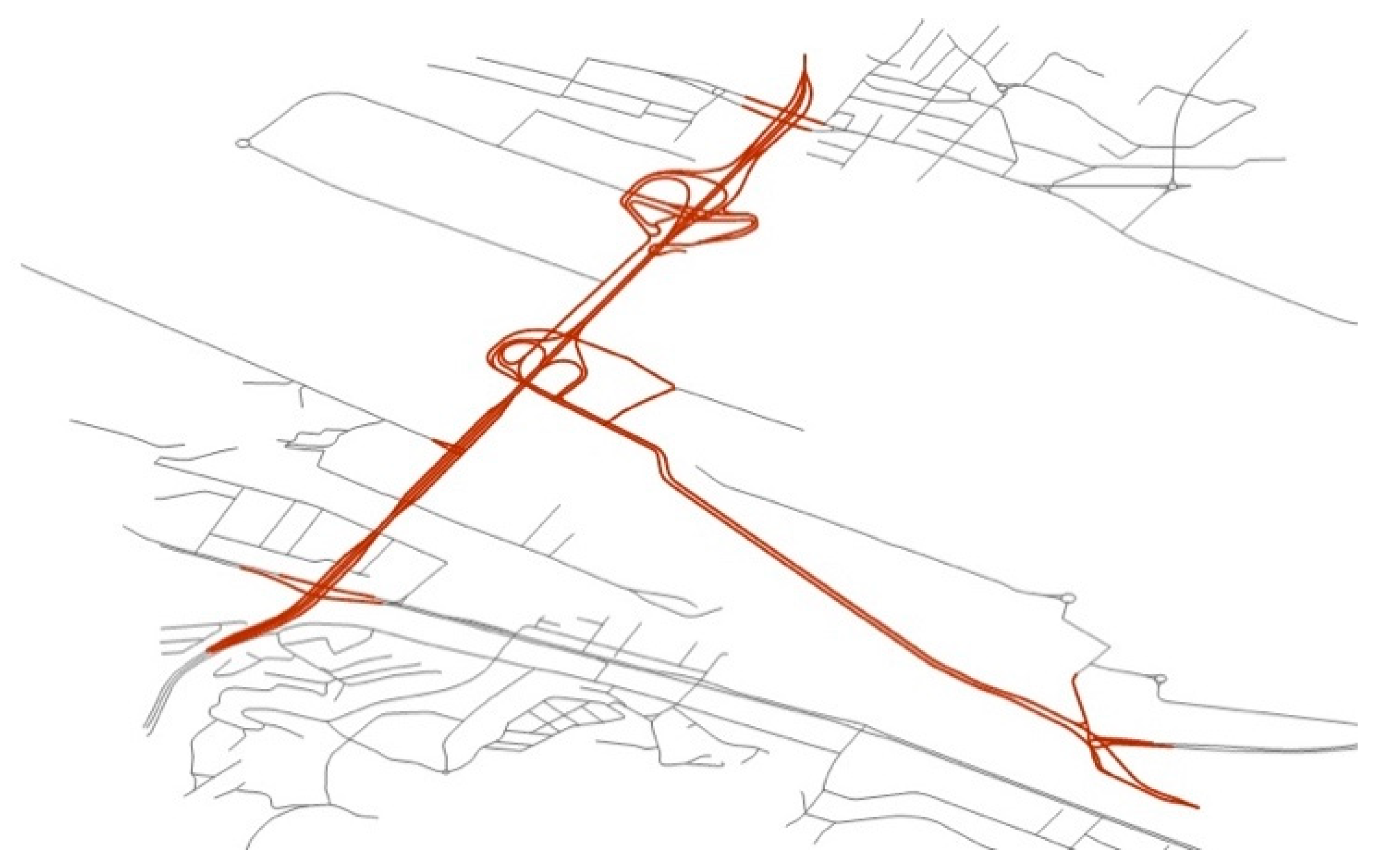
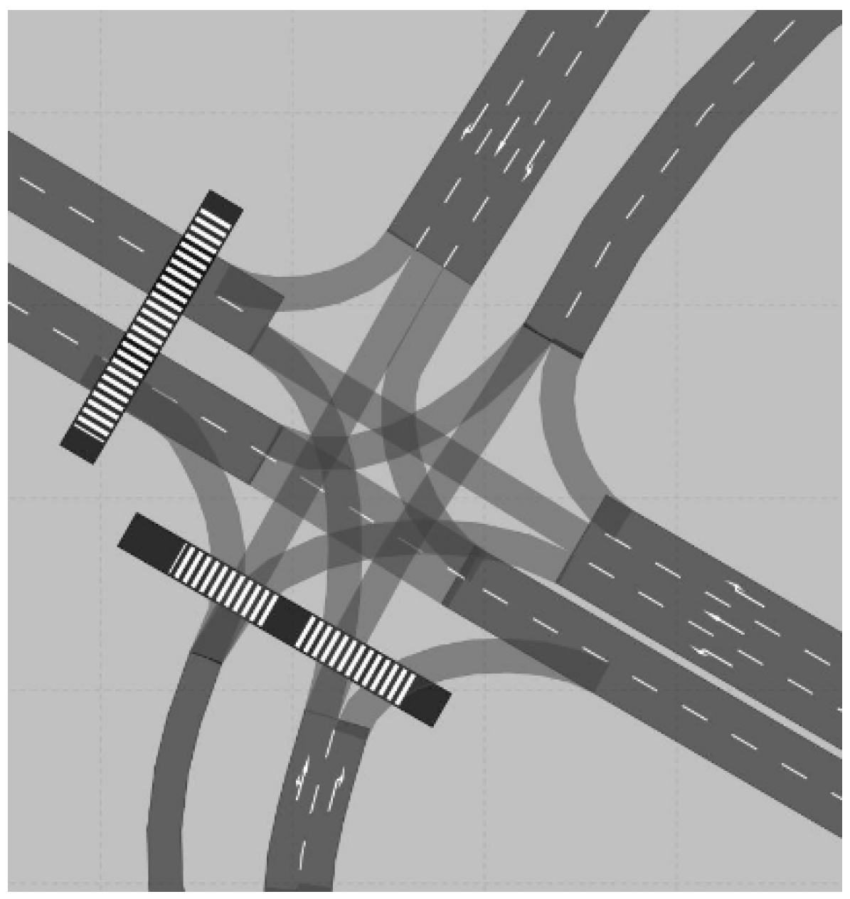
2. Materials and Methods

It is a well-known division of transport models due to the scope of the male territory [30]: macroscopic, mesoscopic, microscopic, and submicroscopic. Such a classification of models allows for a different level of aggregation, level of accuracy, and analogies to other fields of science such as fluid mechanics or gas kinematics. Depending on the result that the researcher wants to obtain, he should adjust the selection of quantities describing given traffic. Other necessary dependencies will be needed for directly related research with planning, for example, traffic flows and their structure [31]. On the other hand, from the point of view of people managing the traffic, e.g., in the traffic control and management center, the most important external data will be the number of vehicles, the method of control or its lack, as well as the organization of traffic at nodes and sections between nodes [32]. Simulation modeling of transport systems and processes has been used for many years, scientific publications relating to the modeling of port management and its transshipments can be found as early as 1980 [33]. Many issues related to the movement of individual units—means of transport—and cargo handling operations were analyzed through the use of complex simulation models due to the extensive and complex processes taking place during their duration. Vehicle traffic in the urban transport network can be analytically modeled, especially for medium and large-scale cases, using many tools specially designed for this. Due to the heterogeneity of vehicle traffic, it is not possible to fully reproduce using the model of all drivers’ behaviors or incidental situations having a direct impact on road traffic [34].

The model used in this publication is on a microscopic scale [35,36]. The data for the analysis was obtained using the PTV Vissim tool [37,38,39,40]. Modeling functionality with the PTV Vissim tool is achieved by entering data on the size of the traffic flow, its type, generic structure, important elements of the road infrastructure (curvature, horizontal, and vertical curves, or the width of the lane), important elements of infrastructure related to public transport, or mapping places related to the movement of pedestrians. The conducted micro-simulation analysis allows for obtaining basic result data in the modeled transport network in a specified time interval, such as queue lengths, travel times, time losses, the number of stops, travel speed, exhaust emissions, or fuel consumption [41,42,43,44,45,46].

To carry out the analysis, as a case study of the impact of heavy goods vehicles on the urban transport network, a model was implemented that reflects the existing state on the example of the port city of Gdynia. The model is valid as of 2 October 2020. Later possible changes to the modeled network or the method of traffic management were not taken into account. The existing condition of the modeled network was compared to the increased volume of heavy goods vehicle traffic resulting from travel to and from the port. The model is designed to check the periods in which the level of freedom of movement will not be exceeded in terms of operational reliability. Particular operational reliability limits for individual states were determined based on the existing state model. To perform the described analysis, a simulation model was created in the PTV Vissim program. This model was supplied with actual data received from the Gdynia Road and Greenery Authority in Gdynia and manually calculated data. The data comes from the TRISTAR (Intelligent Traffic Control System). The peak hour data was additionally measured manually to calibrate the model with the exact generic structure of the vehicles. Due to the measured data on traffic flow at intersections, the model calibration method was selected using the GEH [41,42] indicator. I used this method for each type of vehicle separately due to the result in the unit of vehicles per hour. The basic assumption of the method is to validate and calibrate the model to obtain no more than a 5% difference in the measurement results. An example of a transport network close to the port is a section of the network in the city of Gdynia. The map below shows the scope of the modeled section of the urban transport network of Gdynia city—Figure 1. On red color is marked analyzed road network.

To measure the pollutants emitted, the model lists five intersections where the model measurements took place. These intersections differ in geometry as well as in the generic structure of vehicles. Figure 2, Figure 3, Figure 4, Figure 5 and Figure 6 below show the geometry of the analyzed junctions together with the geoinformation.

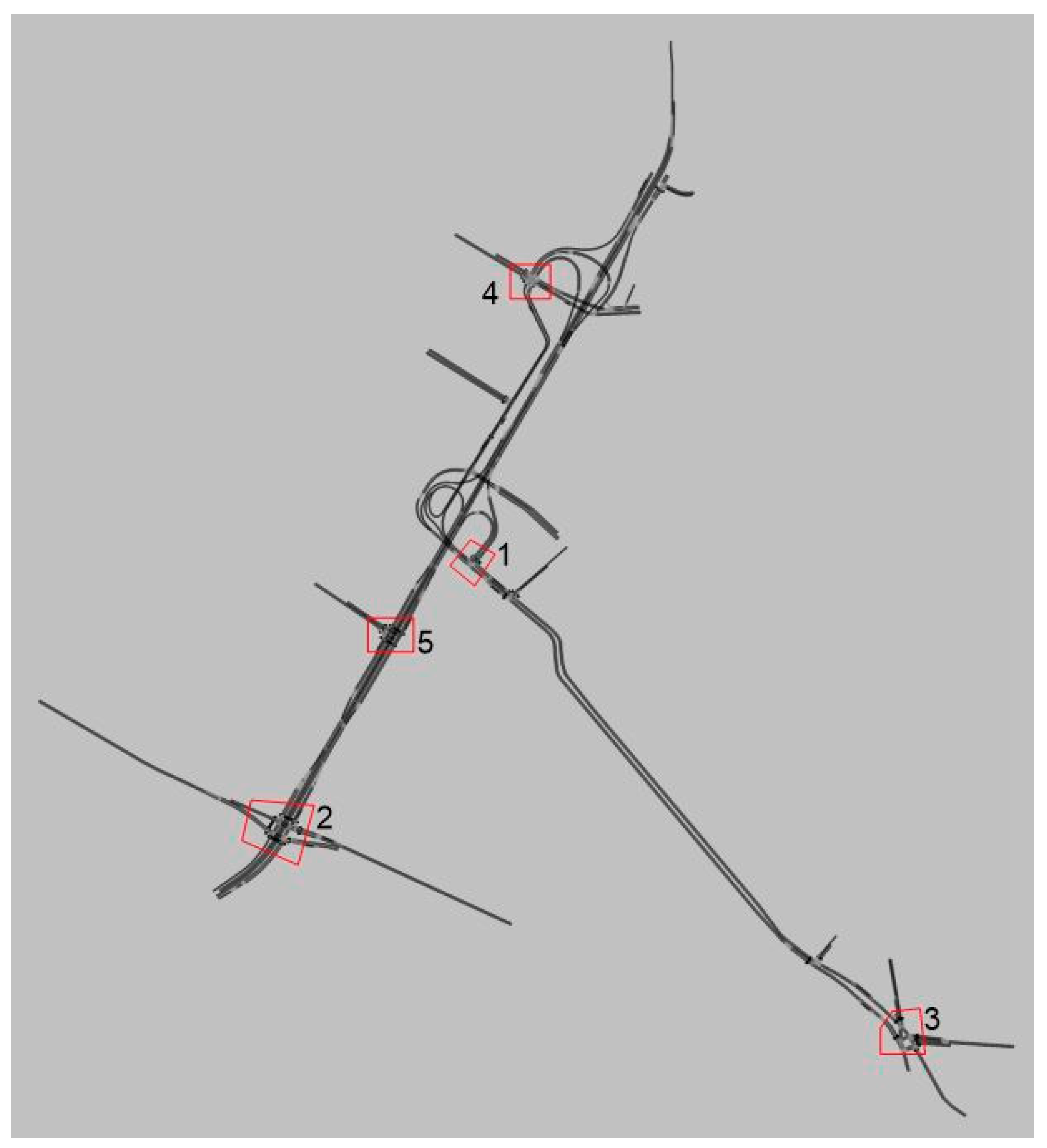
• Junction 1 (54.540335, 18.497963)

Figure 2. Junction 1–3-way intersection Kwiatkowskiego Street/Wiśniewskiego Street.

Figure 2. Junction 1–3-way intersection Kwiatkowskiego Street/Wiśniewskiego Street.

• Junction 2 (54.532896, 18.488618)

Figure 3. Junction 2–4-way intersection Kwiatkowskiego Street/Morska Street.

Figure 3. Junction 2–4-way intersection Kwiatkowskiego Street/Morska Street.

• Junction 3 (54.526868, 18.518786)

Figure 4. Junction 3–4-way intersection Wiśniewskiego Street/Polska Street.

Figure 4. Junction 3–4-way intersection Wiśniewskiego Street/Polska Street.

• Junction 4 (54.548291, 18.500745)

Figure 5. Junction 4–4-way intersection Kontenerowa Street/Kwiatkowskiego Street.

Figure 5. Junction 4–4-way intersection Kontenerowa Street/Kwiatkowskiego Street.

• Junction 5 (54.538310, 18.494027)

Figure 6. Junction 5–3-way intersection Kwiatkowskiego Street/Hutnicza Street.

Figure 6. Junction 5–3-way intersection Kwiatkowskiego Street/Hutnicza Street.

On a microscopic scale, for simulation analysis, for example, the PTV Vissim [43] tool is used. The program allows you to create traffic analyzes road (including individual car, bicycle, and collective traffic), and pedestrian traffic. The tool also allows for the simulation study of mutual interactions generated by groups of traffic users moving on the same road network. In the case of the PTV Vissim tool, the simulation is based on the Wiedemann model associated with the name of “driving behind the leader” because the vehicle following another vehicle reaches its maximum speed then it slows down and accelerates to keep a safe distance from the vehicle in front of it [45]. In order to implement the model, the following activities were made:

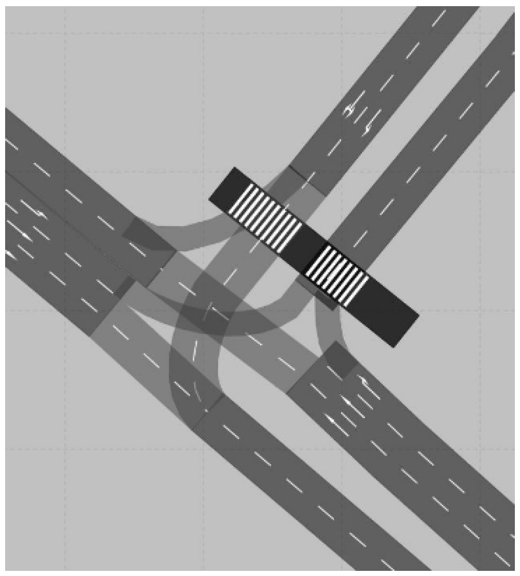
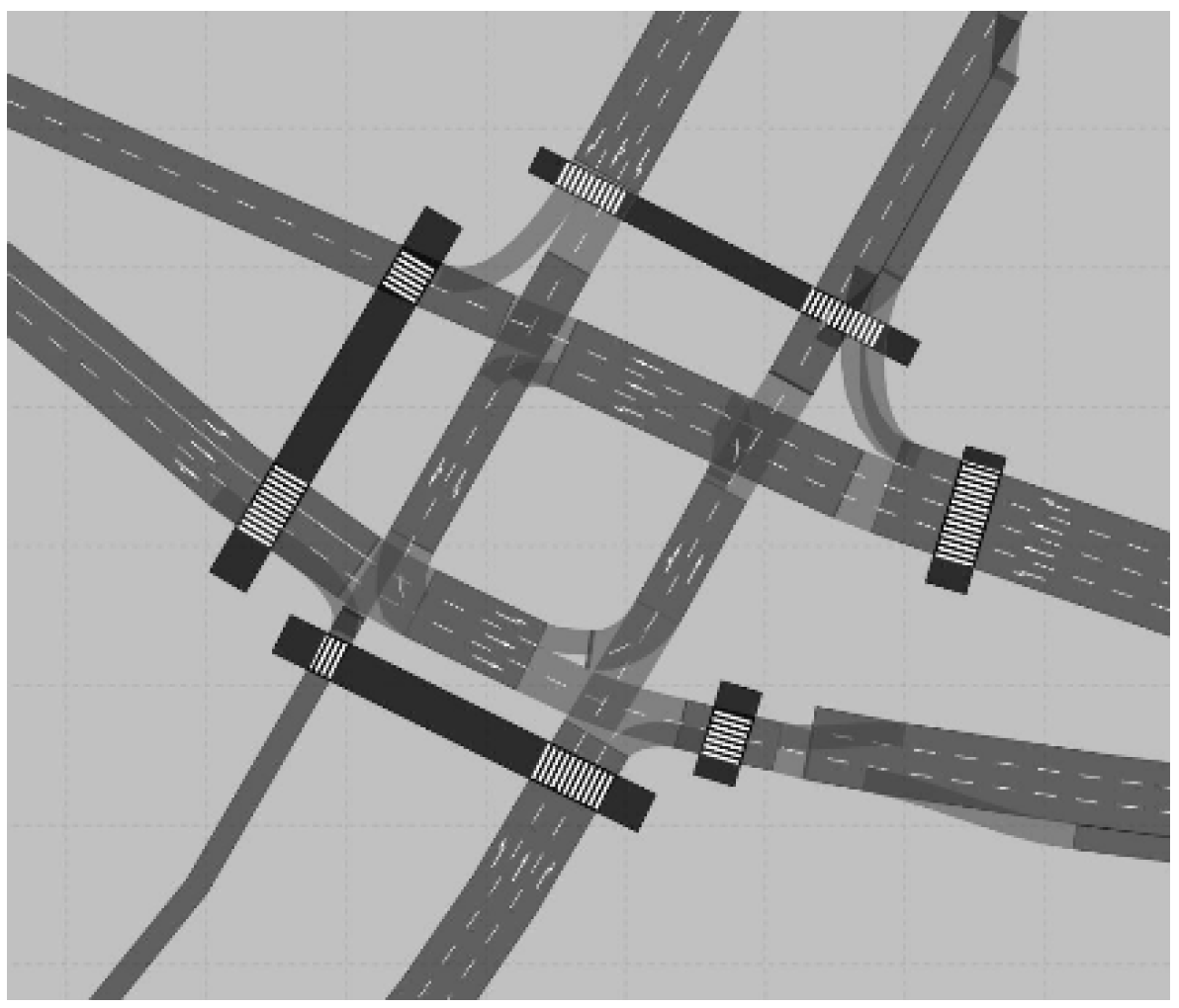
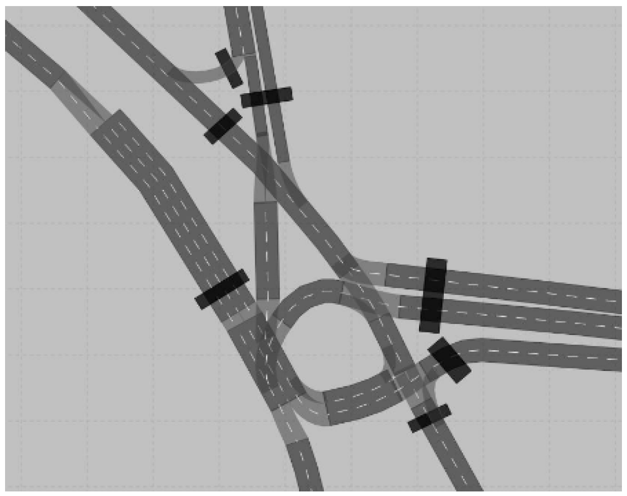
• The road network with the connection system was mapped, orthophotos were used, as well as official data in the case of the height of the modeled flyover;
• Added vehicle loads on an hourly basis from 06:00 to 20:00, data was measured by ITS system Tristar, and manually;
• The generic structure of vehicles was added;
• Torsional relations were added at each intersection with the specified percentage;
• Traffic light programs were added for the period from 06:00 to 20:00 along with the schedule of changing programs depending on the time;
• Traffic lights at intersections;
• Public transport timetables were added, as well as infrastructure such as bus stops, waiting for places for pedestrians;
• Allowable speeds on individual sections were assigned;
• Speeds on torsional relations within the intersection were limited;
• Traffic was assigned and prioritized in disputes;
• Pedestrian traffic was added;
• Measurement points were added;
• Calibrated and validated by the GEH index [46].

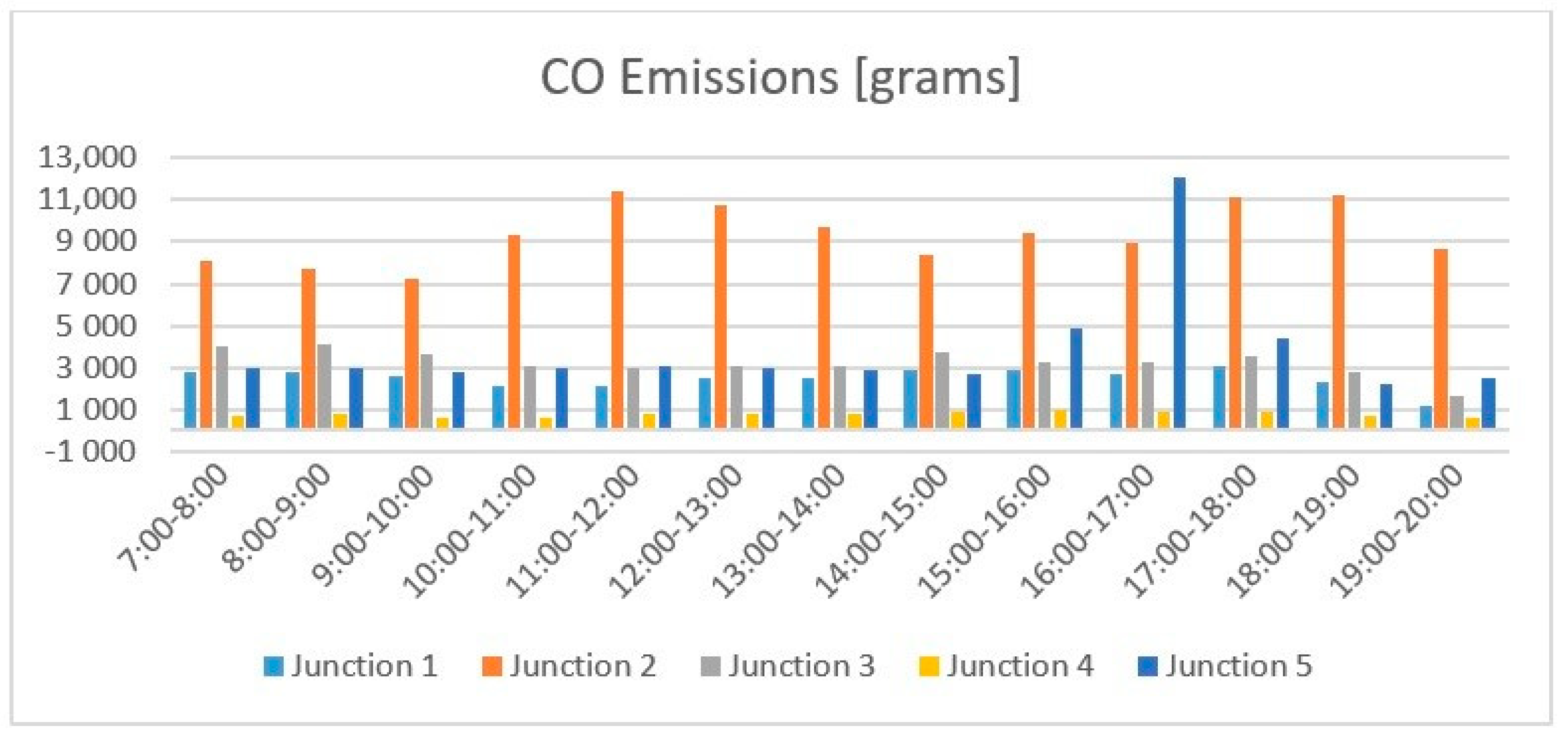
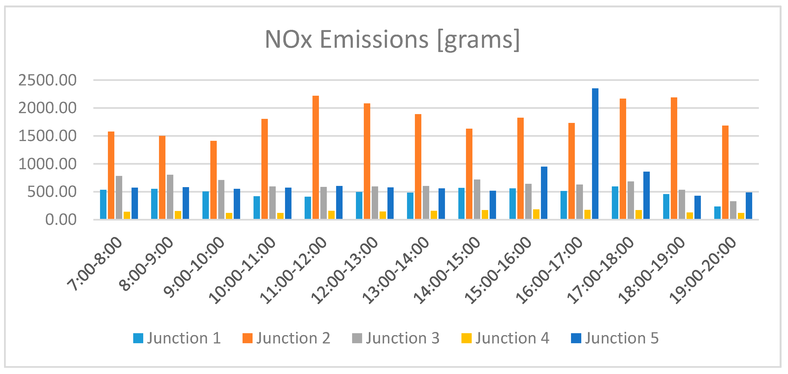
Based on ten simulation runs with the use of random seed 47, the results presented in individual variants are average results. The model made in this way reflected the existing state of the urban road network. In the further part of the work, it was described as Variant 0. The other variants of the model 1, 2 …, 10 reflect the increase in the number of heavy goods vehicles generated by port areas, at three generator points by 10%, 20%, … 100% more concerning the Variant 0.

3. Results

The simulation results were presented based on the analysis of five intersections with traffic lights. The analysis of nodes allowed us to obtain data on the generation of CO [46], NOx [47], VOC [48] by vehicles as well as statistics of fuel consumption [49]. Figure 7 below shows the location of the analyzed intersections in the network. The attached map lists five intersections marked as nodes with numbers from 1 to 5. Impact of the increase in the number of heavy goods vehicles generated by terminals on fuel consumption and pollution in the city. The analysis was divided into variant 0—showing data on the current state, and into other variants with the increased traffic of heavy goods vehicles.

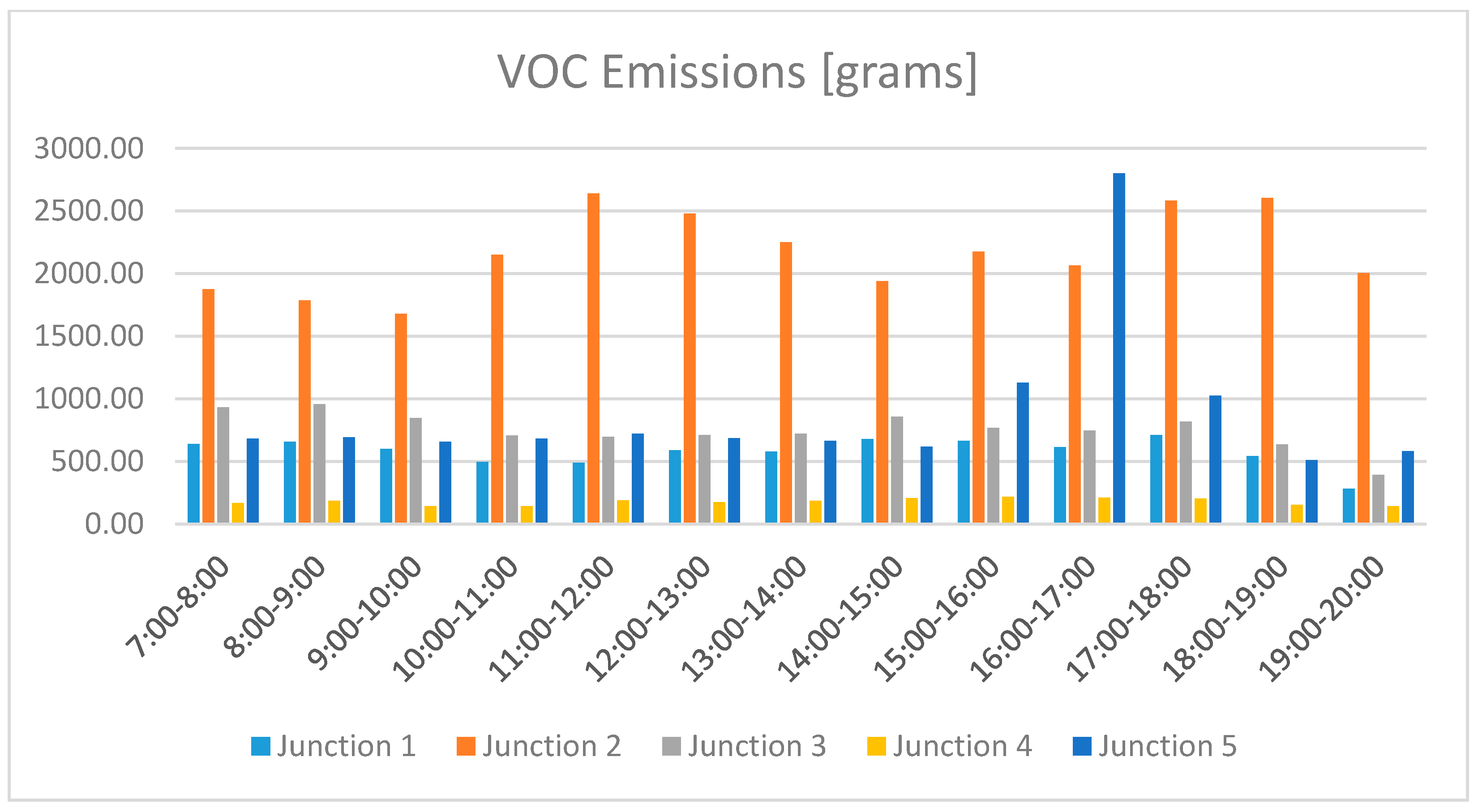
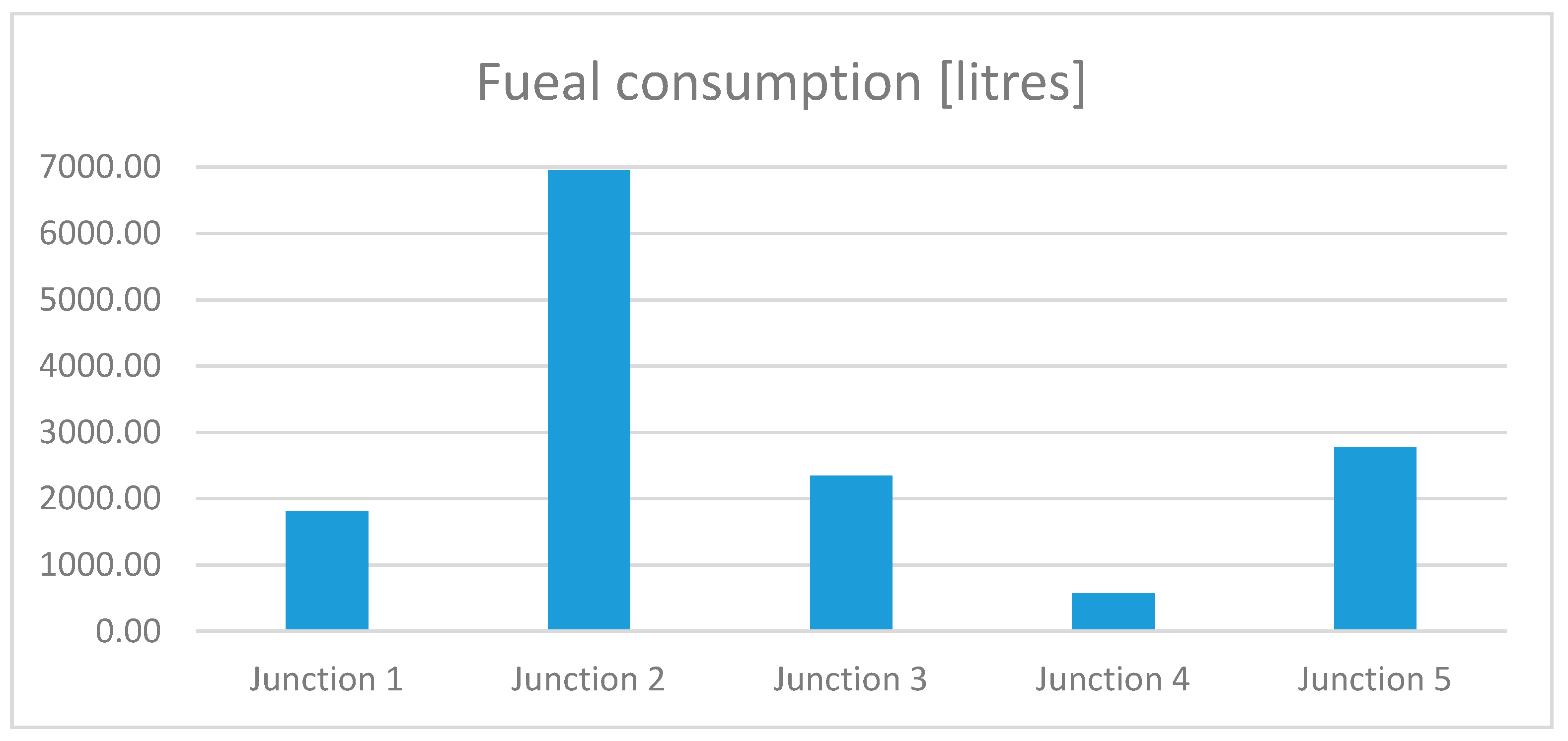
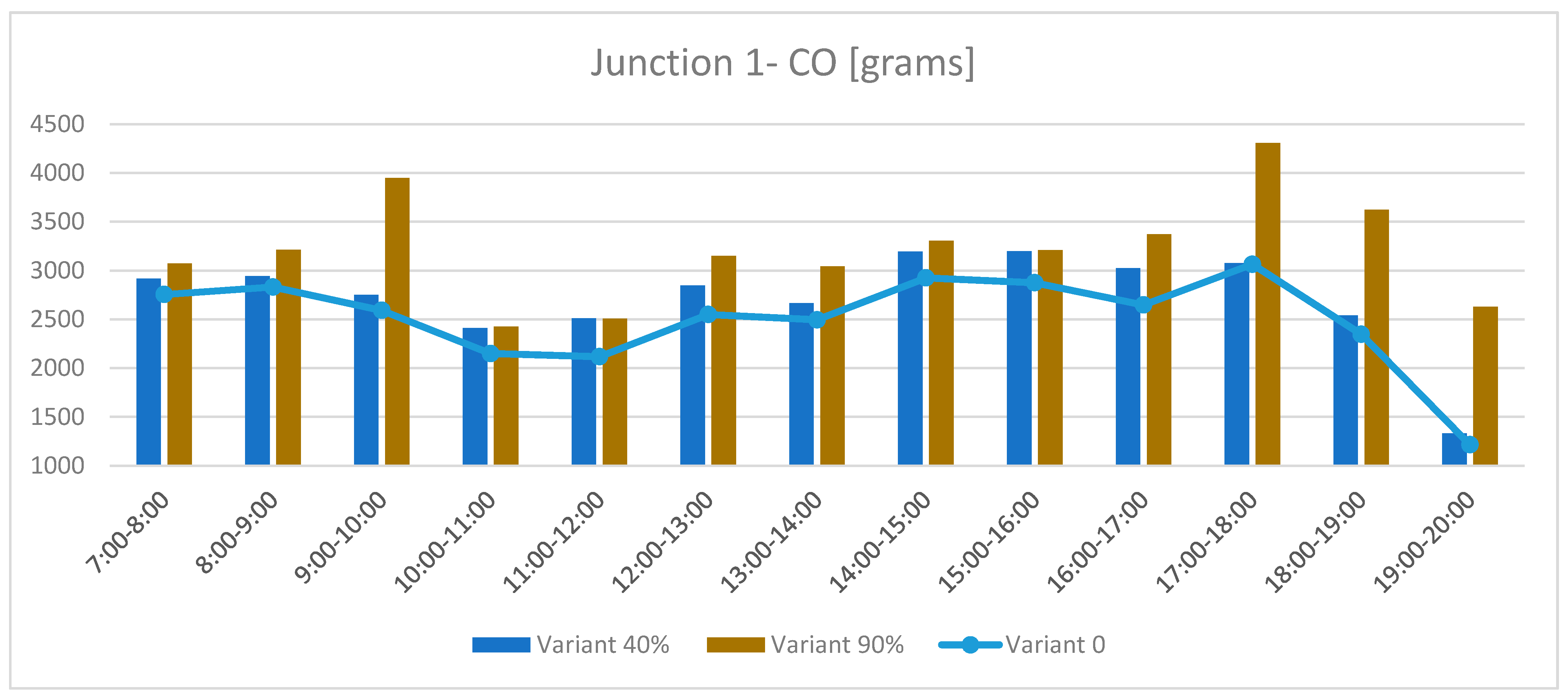
3.1. Variant 0—The Existing State

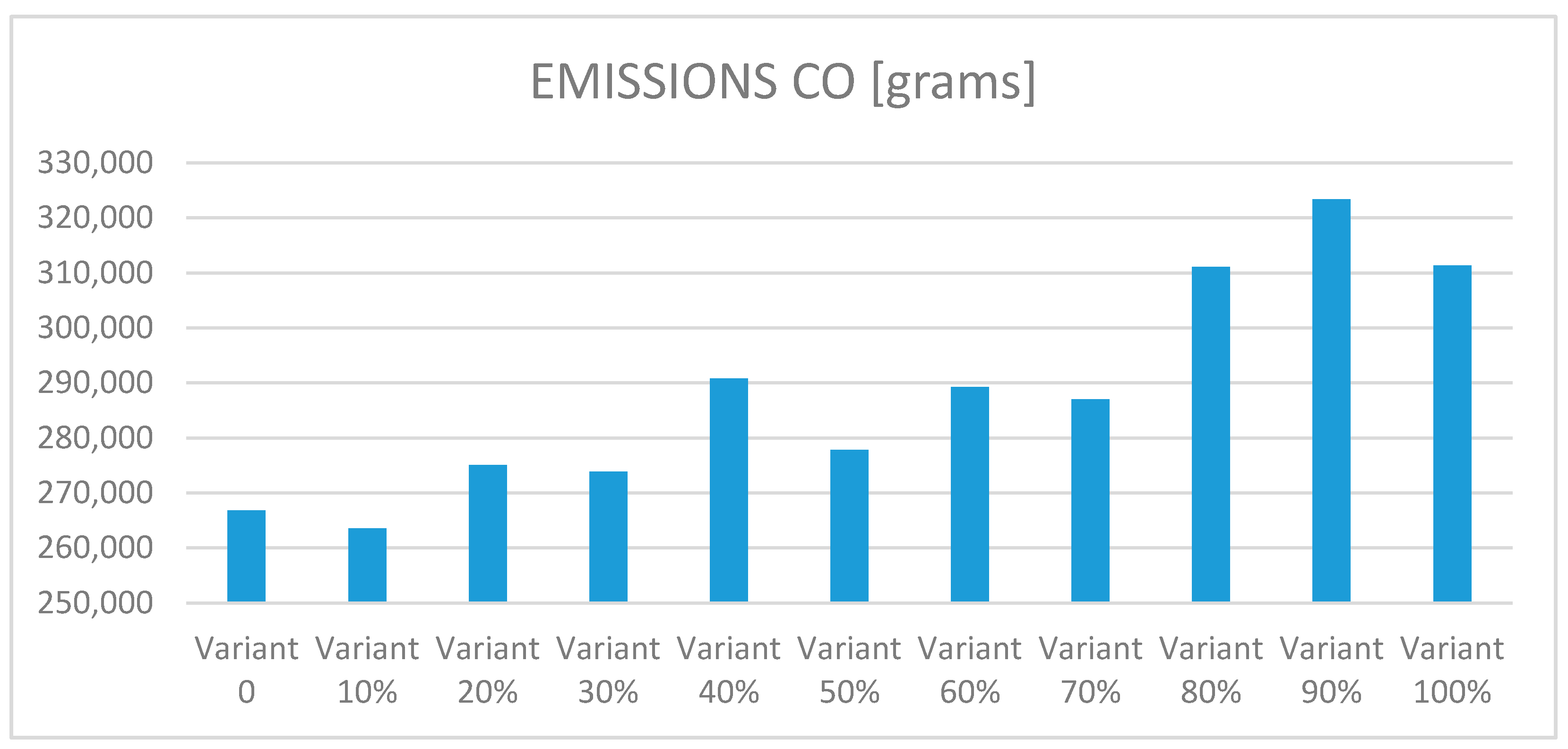
In the results of the Variant 0 microsimulation model, it can be seen that the results differ depending on the junction. It depends on the traffic volume, left turn, the number of stops at an intersection, or the length of the queue at the entrance. Each of the intersections is also located at a different distance from the generator points—port terminals. The extent of CO pollution from a vehicle is startlingly different. In the case of intersection no. 2, the maximum values reach almost 12,000 g during the hour under study. However, in the case of intersection no. 4, these values never exceed 1000 g. In the case of intersection no. 5, the highest emission takes place during the afternoon rush hours, the values reach the value of 12,000 g at the measurement hour. Figure 8 shows the hourly distribution of CO emissions at individual intersections.

In the case of NOx emissions, similarly to CO, the highest emission was measured at junction no. 2, where the maximum value exceeds 2100 g during four measuring hours. Moreover, by analogy with CO, junction 5 generates the highest NOx emissions during the afternoon rush hour from 16:00 to 17:00. Junction no. 4 has incomparably lower values than the other intersections. Figure 9 below shows a graph of NOx emissions broken down by measuring hours.

Similar to the previous data, the highest VOC emission is generated by crossing 2. The measured value exceeds 2500 g three times during the measuring hours. During the afternoon peak, during one measurement hour from 16:00 to 17:00, intersection no. 5 generates the most VOC above 2600 g. At the remaining intersections, the values are emitted at an equal level throughout the post-air period. The distribution of measurement data is shown in Figure 10.

In the case of fuel consumption at individual intersections, also intersection no. 2 consumes almost 7000 L during the calculation period from 7:00 to 20:00. The lowest fuel consumption, and thus environmental pollution, is at the conjunction no. 4—571 L. On the other hand, intersections 1 and 3 generate fuel consumption of about 2000 L. Drivers at junction 5 burn less than 3000 L. Figure 11 shows the variation in fuel consumption at particular intersections.

Measured by value, they are the basis for observing changes while increasing the number of trucks generated by ports.

3.2. Variants 1–10

The results of the micro-scale simulation of variants in which the load of heavy goods vehicles at generator points was increased show that increasing the number of vehicles by 20% brings the first negative effects. Analyzing the sum of the total emission of harmful substances during the measurement period, it was an increase by 40% that showed that there will be an increase in CO by over 20,000 g. The highest emission of harmful substances will occur when the number of heavy goods vehicles through the ports is increased by 90%—the CO emission will exceed 320,000 g during the measurement period. Figure 12 shows a comparison of all variants depending on the increase in the number of heavy goods vehicles.

Referring to variant 0 and then to the one where the number of HGV was increased by 40% and then by 90%, it can be seen that the increase in changes in CO emissions is not linear. These changes are visible mainly during the morning and afternoon peaks. In the mornings from 9:00 am to 10:00, with the intensity of heavy goods vehicles increased by 90% at generator points, exhaust emissions will be almost 1500 g higher than for the other variants during one measurement hour. The increase by over 1000 g will also take place during the afternoon rush from 16:00 to 20:00. Figure 13 shows the hourly CO junction 1 case analysis.

When analyzing the individual sums of exhaust emissions and fuel consumption concerning a specific variant, it should be noted that the changes do not occur in any linear way. Due to the extensive road network, equipped with various variable elements such as intersections, pedestrian crossings, and signaling program, the simulation results will not increase steadily with the increase in the number of vehicles. The use of a micro-simulation tool will allow estimating the deterioration of both road traffic conditions and, above all, air pollution-related to the transport of cargo from the port by road transport. These changes are felt mainly by the inhabitants of the nearby areas adjacent to the port area.

Table 1. Variants comparison—results.

	Emissions CO [g]	Emissions NOx [g]	Emissions VOC [g]	Fuel Consumption [L]
Variant 0	266,842.0	51,917.7	61,843.2	14,450.7
Variant 10%	263,597.8	51,286.6	61,091.3	14,275.0
Variant 20%	275,056.3	53,516.0	63,746.9	14,895.6
Variant 30%	273,860.4	53,283.3	63,469.8	14,830.8
Variant 40%	290,809.7	56,581.0	67,398.0	15,748.7
Variant 50%	277,846.1	54,058.8	64,393.5	15,046.7
Variant 60%	289,245.4	56,276.6	67,035.4	15,664.0
Variant 70%	287,013.0	55,842.3	66,518.0	15,543.1
Variant 80%	311,094.1	60,527.6	72,099.1	16,847.2
Variant 90%	323,418.2	62,925.4	74,955.3	17,514.6
Variant 100%	311,325.7	60,572.7	72,152.7	16,859.7

presents a comprehensive comparison and summary of the results of the case study of an increase in the number of trucks at generator points on the municipal transport network in terms of CO, NOx, VOC emissions, or fuel consumption.

4. Discussion

Traffic modeling is the research field of many disciplines, used in the theory of traffic flow in road networks in the case of addressed microscopic, mesoscopic, and even microscopic traffic simulation. Transport analyses performed by engineers are the basis for making infrastructure decisions by city managers. Typically, in terms of the entire city, macroscopic models are used, which will be able to determine the most important changes depending on the compared variants. The analysis made for this article shows how important the analysis is also on a microscopic scale. This case study of the port of Gdynia and the roads leading to and from the port shows the use of micro-scale models and tools.

The data available in the literature on port analyzes usually show the port in terms of region or country. This is a reasonable approach due to the fact that the port is an important part of the economy of a given country. As a whole, the increase in transshipment through the port brings a positive result for the city or even the region, the port brings huge profits for the city and is also a workplace for many residents. Increasing transshipments will be synonymous with the need to increase work in the port. However, it should be remembered that each cargo must somehow leave the port. However, as in the analyzed case, residents have to share the road infrastructure with loads going to or leaving the port. The performance of the described analysis will allow estimating the negative impact of the increase in the number of trucks generated by the port on the lives of residents.

Any increase in the number of vehicles has an impact on the environment. The obtained data from the microsimulation model should be read in a local reference. If the number of heavy goods vehicles is increased, each 10% more vehicles generated by ports will have an impact on the deteriorating traffic conditions in the port city. The microscopic analysis presented in this article shows what negative effects should be expected in the case of increasing the loading capacity of a given food. It should also be noted that there is a possibility of mitigating the negative effects by using rail or inland transport for the further transport of cargo from the port. Local authorities should therefore strive not to exceed the limit values for the number of vehicles, especially heavy goods vehicles, in urban areas. An important factor in promoting sustainable transport or urban transport to reduce exhaust emissions.

The analysis presented in the article can be used in any port area, only with the need to perform and calibrate the micro-simulation model. Due to the different road networks in each city, the results will be different, however, the measurement method can be fully used. In the case of the Gdynia port analysis, the volume of heavy goods vehicles by 40% will cause significant changes in road traffic, the number of exhaust gases, and fuel consumption.

5. Conclusions

This analysis shows the possibility of using a micro-simulation tool to reflect the negative environmental impact of vehicles through exhaust emissions.

The pursuit of modern cities towards sustainable development, both economically and ecologically, should form the basis of the future activities of local authorities. The definition of limit values that city authorities should not exceed may be determined based on the study presented in this article. On the example of the Gdynia city—on the analyzed section of the network, the pollution by exhaust gases differed depending on the measuring point. Due to numerous factors influencing the measurement, such as the number of vehicles, type of vehicle, number of stops, free movement, and the results are not linear. In the analyzed case, an increase of the number of road transport by 40% resulted in a significant increase in exhaust gas emissions. It should be noted that the study was performed daily. Thus, the obtained CO increase of 20,000 g in the case of a 40% increase in the number of vehicles generated by the port daily will generate about 600 kg of CO emissions monthly only at one intersection. Monitoring of exhaust gases in cities, and especially in industrial cities, e.g., port cities, is an essential element to provide residents with a healthy and safe place to live.

The presented case study can be applied to any road network in the vicinity of any port. The analysis can only be performed on a well-constructed and then calibrated microsimulation model.

The impact of the port on the port city is inevitable. Micro-scale analysis is able to show when there is a significant deterioration in traffic conditions and an increase in exhaust emissions. PTV Vissim is useful because it allows you to map the network in every detail. These details are important due to the road network which varies from place to place. The key application of the article is for city management to supervise and control the level of pollution in the city in the future. A model is a useful tool for the prediction of pollution as well as for determining the limit state which should not be exceeded. In the analyzed case, an increase in heavy goods vehicles by 40% compared to the existing state will significantly increase the pollutants emitted into the environment. The described example can be applied to any other case. However, it has limitations in the form of a paid license for the PTV VISSIM software. Another limitation is the need to have actual data to correctly estimate the amount of pollution generated by vehicles.

References

1. Żochowska, R. Modelowanie wyboru trasy w gęstych sieciach miejskich. Zesz. Nauk. Transp. Politech. Śląska 2011, 71, 97–109. [Google Scholar]
2. Żochowska, R. Dynamic approach to the Origin-destination matrix estimation in dense street networks. Arch. Transp. 2012. [Google Scholar] [CrossRef]
3. Anagnostopoulos, C.-N. Modeling Transport, 4th Edition. IEEE Intell. Transp. Syst. Mag. 2012. [Google Scholar] [CrossRef]
4. Islam, T.; Akhie, A.A.; Amin, M.S.; Amit, S.K. Validation of Vissim for Capacity Estimation of Highway. In Proceedings of the 2nd International Conference on Research and Innovation in Civil Engineering (ICRICE-2020), Chittagong, Bangladesh, 12–13 January 2018. [Google Scholar]
5. Nadanakumar, V.; Muthiya, J.; Prudhvi, T.; Induja, S.; Sathyamurthy, R.; Dharmaraj, V.; Joseph, J. Experimental investigation to control HC, CO & NOx emissions from diesel engines using diesel oxidation catalyst. Mater. Today Proc. 2021, 43, 434–440. [Google Scholar] [CrossRef]
6. Alsultan, A.; Mijan, N.; Mansir, N.; Zulaika, S.; Yunus, R.; Taufiq-Yap, Y.H. Combustion and Emission Performance of CO/NOx/SOx for Green Diesel Blends in a Swirl Burner. ACS Omega 2020, 6, 408–415. [Google Scholar] [CrossRef] [PubMed]
7. Chan, C.-C.; Nien, C.; Hwang, J.-S. Receptor modeling of VOCs, CO, NOx, and THC in Taipei. Atmos. Environ. 1996, 30, 25–33. [Google Scholar] [CrossRef]
8. Gorbik, Y.; Kashkanov, A.; Antoniuk, O. Method of diagnosing a car by fuel consumption. J. Mech. Eng. Transp. 2021, 12, 45–53. [Google Scholar] [CrossRef]
9. Nævestad, T.-O.; Sagberg, F.; Levlin, G.; Bjørnskau, T. Competence, equipment and behavioural adaptation on Norwegian winter roads: A comparison of foreign and Norwegian HGV drivers. Transp. Res. Part F Traffic Psychol. Behav. 2021, 77, 257–273. [Google Scholar] [CrossRef]
10. Madhusudhanan, A.; Ainalis, D.; Na, X.; Garcia, I.; Sutcliffe, M.; Cebon, D. Effects of semi-trailer modifications on HGV fuel consumption. Transp. Res. Part D Transp. Environ. 2021, 92, 102717. [Google Scholar] [CrossRef]
11. Rys, D.; Judycki, J.; Jaskula, J. Impact of overloaded vehicles on load equivalency factors and service period of flexible pavements. In Proceedings of the 10th International Conference on the Bearing Capacity of Roads, Railways and Airfields, BCRRA 2017, Athens, Greece, 28–30 June 2017. [Google Scholar]
12. Luo, Y.; Chen, J.; Liu, W.; Ji, Z.; Ji, X.; Shi, Z.; Yuan, J.; Li, Y. Pollutant concentration measurement and emission factor analysis of highway tunnel with mainly HGVs in mountainous area. Tunn. Undergr. Sp. Technol. 2020, 106, 103591. [Google Scholar] [CrossRef]
13. Neal, Z.; Derudder, B.; Taylor, P. Forecasting the world city network. Habitat Int. 2020, 106, 102146. [Google Scholar] [CrossRef]
14. Prezes Rady Ministrów Rządowe Centrum Legislacji Rozporządzenie Ministra Transportu I Gospodarki Morskiej z dnia 2 marca 1999 r. w sprawie Rozporządzenie Ministra Transportu i Gospodarki Morskiej z dnia 2 marca 1999 r. w sprawie warunków technicznych, jakim powinny odpowiadać drogi publiczne i ich usy. Dz. Ustaw 2013. Available online: https://bip.rcl.gov.pl/ (accessed on 1 June 2021).
15. Ziemska, M. The idea of using intelligent transport systems and coordination of traffic lights. Pr. Wydz. Nawig. Akad. Morskiej w Gdyni 2014, 29, 107–112. [Google Scholar] [CrossRef] [Green Version]
16. Ziemska, M.; Smolarek, L. Analysis of the effect of mass events on car traffic in the city in the daily interval. In Proceedings of the 2017 2nd International Conference on System Reliability and Safety (ICSRS), Politecnico di Milano, Milan, Italy, 20–22 December 2017; Volume 2018-Janua, pp. 521–525. [Google Scholar]
17. Ziemska, M.; Smolarek, L. The Time Losses as a Reliability of Transport in the Municipal Network during the Mass Event. In Proceedings of the 2019 4th International Conference on System Reliability and Safety, ICSRS 2019, Rome, Italy, 20–22 November 2019. [Google Scholar]
18. Ziemska, M.; Smolarek, L. Modeling the Participation of Heavy Vehicles Stream, Using the System of Automatic Weigh Control of Vehicles in the City of Gdynia. In Proceedings of the 2018 3rd International Conference on System Reliability and Safety, ICSRS 2018, Barcelona, Spain, 24–26 November 2018. [Google Scholar]
19. Gaca, S.; Suchorzewski, W.; Tracz, M. Inżynieria Ruchu Drogowego Teoria i Praktyka, 1st ed.; Wydawnictwa Komunikacji i Łączności: Warszawa, Poland, 2014; ISBN 978-83-206-1888-4. [Google Scholar]
20. Tabachnikova, E. Description of environmental factors influencing sustainability of motor transport companies of different types. Vestn. Astrakhan State Tech. Univ. Ser. Econ. 2021, 2021, 57–65. [Google Scholar] [CrossRef]
21. Koo, B.; Han, K. Estimate the Road Resistance Coefficient of Light Weight Vehicle; SAE Technical Paper 2013-01-0077; SAE International: Bangkok, Thailand, 2013. [Google Scholar] [CrossRef]
22. Belc, F.; Lucaci, G. New Trends in Designing Road Resistance Structures. Sust. In Sci. Eng. 2009, 1, 27–29. [Google Scholar]
23. Just, J.; Maziarka, S.; Misiakiewicz, Z.; Wyszyńska, H. Pojazdy samochodowe i rodzaj nawierzchni jezdni jako źródlo zanieczyszczenia powietrza atmosferycznego substancjami rakotwórczymi i ołowiem. Rocz. Panstw. Zakl. Hig. 1971. Available online: http://agro.icm.edu.pl/agro/element/bwmeta1.element.agro-884ea4e7-4288-4e26-866a-16161d082460 (accessed on 1 June 2021).
24. Woch, J. Kształtowanie Płynności Ruchu w Gęstych Sieciach Transportowych; Polska Akademia Nauk—oddział w Katowicach, Komisja Transportu; Wydawnictwo Szumacher: Kielce, Poland, 1998. [Google Scholar]
25. Sobota, A.; Karoń, G. Postrzeganie warunków ruchu miejskiego—Płynność ruchu—wyniki badań ankietowych. Zesz. Nauk. SITK RP 2009, 90, 215–234. [Google Scholar]
26. Bergel-Hayat, R.; Żukowska, J. Time-Series Analysis of Road Safety Trends Aggregated at National Level in Europe for 2000–2010; Gdańsk University of Technology Publishing House: Gdańsk, Poland, 2015; ISBN 978-83-7348-630-0. [Google Scholar]
27. Jacob, B.; Cottineau, L.M. Weigh-in-motion for Direct Enforcement of Overloaded Commercial Vehicles. Transp. Res. Procedia 2016, 14, 1413–1422. [Google Scholar] [CrossRef] [Green Version]
28. Caprez, M.; Doupal, E.; Jacob, B.; O’Connor, A.J.; O’Brien, E.J. Test of WIM sensors and systems on an urban road. Heavy Veh. Syst. 2000, 7, 169–190. [Google Scholar] [CrossRef]
29. Rys, D.; Judycki, J.; Jaskula, P. Analysis of effect of overloaded vehicles on fatigue life of flexible pavements based on weigh in motion (WIM) data. Int. J. Pavement Eng. 2016, 17, 716–726. [Google Scholar] [CrossRef]
30. Jessup, E.L. An economic analysis of trucker’s incentive to overload as affected by the judicial system. Res. Transp. Econ. 1996, 4, 131–159. [Google Scholar] [CrossRef]
31. Morse, P.M. Introduction to the Theory of Queues. Lajos Takacs. Science 1962, 137, 742–743. [Google Scholar] [CrossRef]
32. Oskarbski, J.; Gumińska, L. The application of microscopic models in the study of pedestrian traffic. MATEC Web Conf. 2018, 231, 03003. [Google Scholar] [CrossRef]
33. Gardziejczyk, W.; Gierasimiuk, P.; Motylewicz, M. Klimat akustyczny w otoczeniu ulic prowadzących ruch tranzytowy pojazdów ciężarowych. In Proceedings of the Metody ochrony środowiska przed hałasem—Teoria i praktyka. Konferencja Transnoise 2013, Zakopane, Poland, 23–25 October 2013. [Google Scholar]
34. Ziemska, M.; Płodzik, E.; Falkowska, M. Comparative analysis of ports practices and activities in the tri-city and China. TransNav 2019, 13. [Google Scholar] [CrossRef]
35. Krośnicka, K.A. Przestrzenne Aspekty Kształtowania i Rozwoju Morskich Terminali Kontenerowych, 1st ed.; Wydawnictwo Politechniki Gdańskiej: Kielce, Poland, 2016; ISBN 978-83-7348-684-3. [Google Scholar]
36. Wang, L.; Xue, X.; Zhou, X.; Wang, Z.; Liu, R. Analyzing the topology characteristic and effectiveness of the China city network. Environ. Plan. B Urban Anal. City Sci. 2021, 239980832098301. [Google Scholar] [CrossRef]
37. Palomo-Navarro, Á.; Navio-Marco, J. Smart city networks’ governance: The Spanish smart city network case study. Telecommun. Policy 2017, 42, 872–880. [Google Scholar] [CrossRef]
38. Gomes, G.; May, A.; Horowitz, R. Congested freeway microsimulation model using VISSIM. Transp. Res. Rec. J. Transp. Res. Board 2004, 1876, 71–81. [Google Scholar] [CrossRef]
39. Maerivoet, S.; De Moor, B. Transportation Planning and Traffic Flow Models; Physics and Society: Ottawa, ON, Canada, 2005. [Google Scholar]
40. Jacyna, M. Modelowanie i Ocena Systemów Transportowych; OWPW: Warszawa, Poland, 2009; ISBN 978-83-7207-808-7. [Google Scholar]
41. Szymanek, A. Sterowanie ruchem w transporcie. Koncepcja podstaw teoretycznych. Zesz. Nauk. Politech. Warsz. Ser. Transp. 1996, 35. [Google Scholar]
42. Tuğcu, S. A simulation study on the determination of the best investment plan for istanbul seaport. J. Oper. Res. Soc. 1983, 34, 479–487. [Google Scholar] [CrossRef]
43. Siddharth, S.M.P.; Ramadurai, G. Calibration of VISSIM for Indian Heterogeneous Traffic Conditions. Procedia Soc. Behav. Sci. 2013, 104, 380–389. [Google Scholar] [CrossRef] [Green Version]
44. Treiber, M.; Kesting, A. Traffic Flow Dynamics: Data, Models and Simulation; Springer: New York, NY, USA, 2013; ISBN 9783642324604. [Google Scholar]
45. Krauß, S. Microscopic modeling of traffic flow: Investigation of collision free vehicle dynamics. D L R—Forschungsberichte Deutsches Zentrum für Luft– und Raumfahrt Hauptabteilung Mobilität und Systemtechnik, Koln, Germany 1998. Available online: https://sumo.dlr.de/pdf/KraussDiss.pdf (accessed on 1 June 2021).
46. Lownes, N.E.; Machemehl, R.B. VISSIM: A multi-parameter sensitivity analysis. In Proceedings of the Winter Simulation Conference, Monterey, CA, USA, 3–6 December 2006. [Google Scholar]
47. Chauhan, B.; Joshi, G.; Parida, P. Speed Trajectory of Vehicles in VISSIM to Recognize Zone of Influence for Urban-Signalized Intersection. In Recent Advances in Traffic Engineering; Springer: Singapore, 2020; pp. 505–516. ISBN 978-981-15-3741-7. [Google Scholar]
48. Lochrane, T.W.P.; Al-Deek, H.; Dailey, D.J.; Krause, C. Modeling driver behavior in work and nonwork zones: Multidimensional psychophysical car-following framework. Transp. Res. Rec. 2015, 2490, 116–126. [Google Scholar] [CrossRef]
49. Kaths, H.; Keler, A.; Bogenberger, K. Calibrating the wiedemann 99 car-following model for bicycle traffic. Sustainability 2021, 13, 3487. [Google Scholar] [CrossRef]
Figure 1. Part of the municipal transport network of the city of Gdynia (18°33′ E, 54°30′ N) was analyzed by simulation modeling.
Sustainability 13 07428 g001
Figure 7. Road network with marked nodes.
Sustainability 13 07428 g007
Figure 8. CO Emissions-Variant 0.
Sustainability 13 07428 g008
Figure 9. NOx Emissions-Variant 0.
Sustainability 13 07428 g009
Figure 10. VOC Emissions-Variant 0.
Sustainability 13 07428 g010
Figure 11. Fuel Consumption-Variant 0.
Sustainability 13 07428 g011
Figure 12. CO variants comparison.
Sustainability 13 07428 g012
Figure 13. Junction 1 CO emission Variant 0, Variant 40%, Variant 90% comparison.
Sustainability 13 07428 g013