
Susceptibility Analysis of Glacier Debris Flow by Investigating the Changes in Glaciers Based on Remote Sensing: A Case Study


Abstract
1. Introduction
- (1)
- We identified the ablation zone by comparing glacier boundaries in 2000 and glacier boundaries in 2015 in the study area near Duku highway;
- (2)
- We calculated ablation volume by changes in glacier elevation and ablation area from 2000 to 2015;
- (3)
- We used the volume of glacier melting in different basins for glacier debris flow susceptibility based on the improved GIE method.
2. Materials and Methods
2.1. Materials
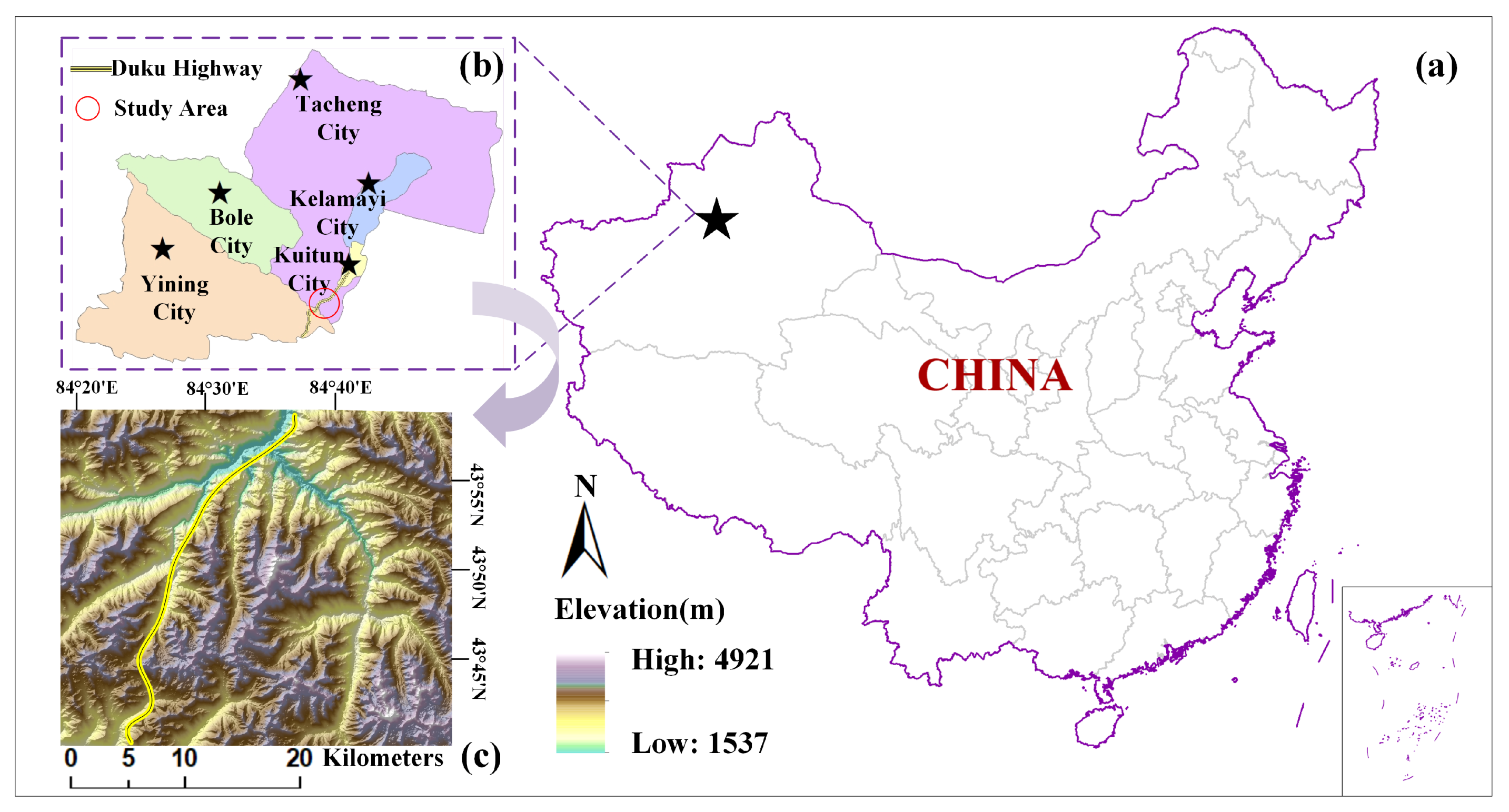
2.1.1. Brief Introduction to the Study Area
2.1.2. Details of the Target Area
2.1.3. Remote Sensing Image Data
2.2. Methods
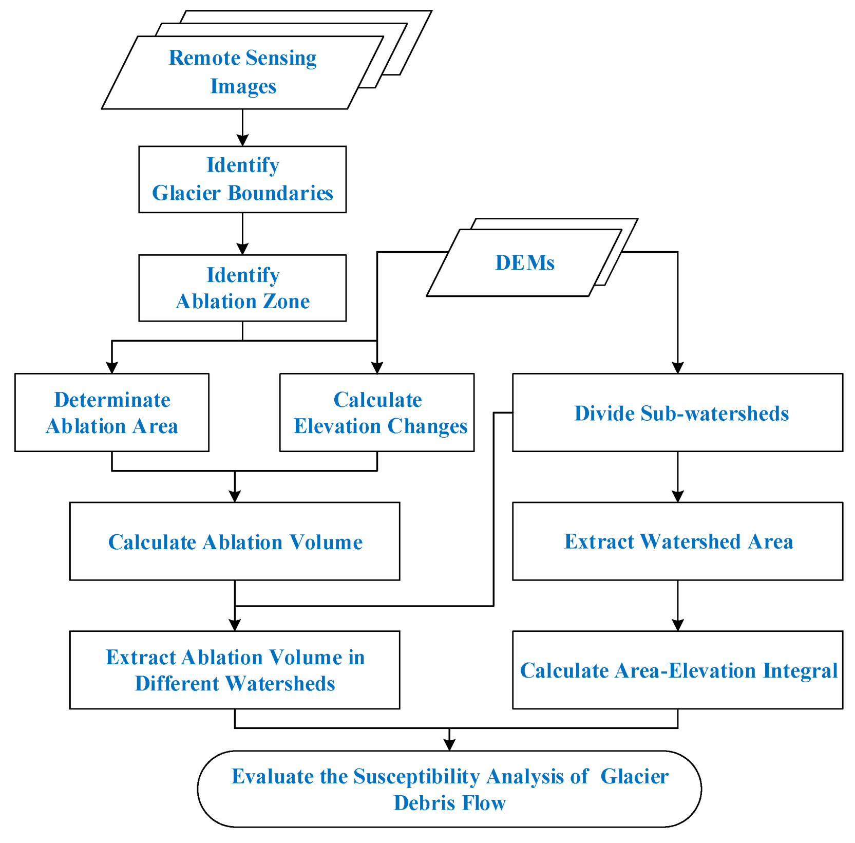
2.2.1. Overview
2.2.2. Step 1: Identification of Ablation Zone
- (1)
- Pre-processing of the Remote Sensing ImagesDue to the interference of solar radiation, clouds, topography, etc., it is necessary to preprocess remote sensing images to avoid the loss in the process. These steps of remote sensing image preprocessing included radiometric calibration, atmospheric correction, geometric correction, and image sharpening of Gram-Schmidt (GS) pan sharpening. These steps can reduce the impact, like noise and improve the quality of images before the classification operation.
- (2)
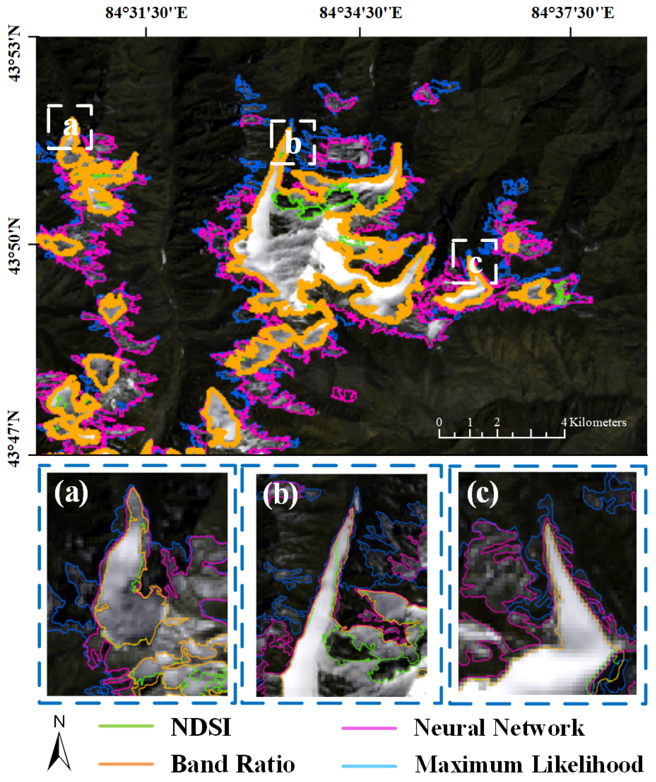
- Main Processing: Identification of Glaciers BoundariesSatellite data have been commonly used for glacier outline identification. For example, by stereoscopic interpretation with aerial photo and Landsat TM data, Aniya, M. [31] identified glacier boundaries and glacier watersheds. Gjermundsen, E.F. [32] calculated the changes of glacier area and extracted the 2002 glacier boundaries in the central Southern Alps, New Zealand. Accurate glacier boundaries are quite important to the study of glacier changes. When glacier extents are regarded as a primary factor for change analysis, it is essential to know how accurate they are. Therefore, it is necessary to obtain with the manual correction of the original outlines (e.g., for debris cover, shadow) [32]. Creating an automated glacier-mapping method that is compared with digital boundaries can be calculated for selected glaciers in the study area. The identification of glacier boundaries based on satellite data was inspired by related work.Among the methods for glacier classification, the common method is the simple band ratio method, which has a fast speed, high precision, and great robustness. A number of studies on glaciers are based on this method. For example, Andreassen, L.M. [28] obtained glacier mapping by threshold ratio images (TM3/TM5). Le Bris, R. [33] used this method based on an application of a threshold (TM3/TM5) to automatically map accurate glacier outlines through the manual correction of misclassified lakes in the study area.This method calculates the reflectance ratio between two bands. The basic principle is to use different reflectivities for different wavebands to distinguish glaciers from other ground objects. The accuracy of this method depends on the selection of thresholds. There are other commonly-used methods, such as NDSI, the maximum likelihood method, and the neural network method. NDSI is computed as (Green-SWIR)/(Green+SWIR) for extracting glacier extents. The maximum likelihood method and the neural network method generally belong to the algorithms of supervised classification, which classify new sample pixels by establishing a typical training sample [34].As illustrated in Figure 4, it shows different glacier boundaries based on the four methods. The classification results of these methods are as follows. Due to the NDSI method has low recognition of moraine-covered glaciers [35,36], it is easy to identify bare land as glaciers, and the results of glacier classification are fragmented. The maximum likelihood method misclassifies rivers as glaciers [37]. In addition, it is easy to misclassify snow and bare land as glaciers, causing the salt-and-pepper phenomenon. The maximum likelihood method is easy to misclassify snow as glaciers, and the classification results are also fragmented. The neural network method is more accurate than the maximum likelihood, while the training time of this method for samples is relatively long, and in this case, the snow, bare land, and glaciers cannot be well-identified. Although the band ratio method creates some cavities inside the glacier with a too small threshold, it can be solved by adjusting multiple times on the selection of thresholds according to the actual situation. Among the four methods, the simple band ratio method is the most suitable in this study. The results based on Red/SWIR for classification are better than those based on NIR/SWIR after testing.
- (3)
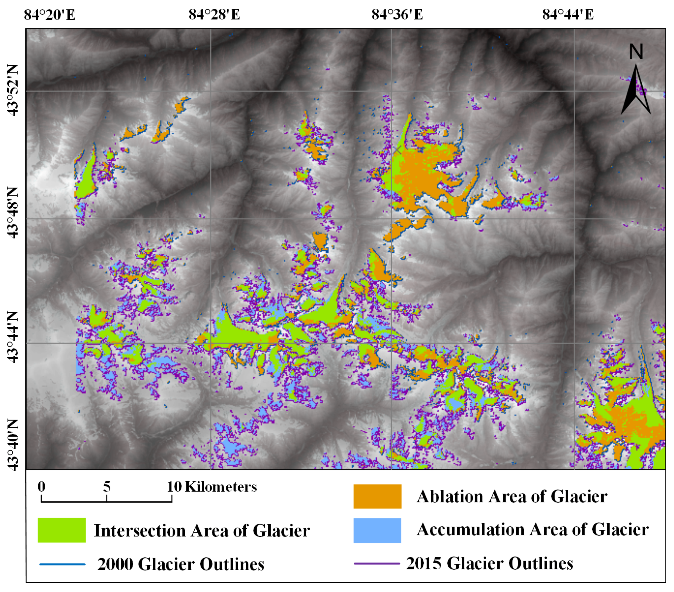
- Post-processing of the Glaciers BoundariesIn the results of automatic classification of glaciers based on remote sensing images, there are usually many small patches or holes. Thus, we need to manually correct interpretation of glacier outlines after the classification operation is implemented. These patches can easily be selected and deleted in the layer by manual editing to improve the accuracy of the glacier outlines. Furthermore, the automatic classification method of glaciers can lead to the misclassification of glaciers (e.g., snow cover, rivers, and clouds). The proper correction of glacier boundaries can use high-resolution images, such as Google Earth images, Landsat series data by overlay of three individual bands, and even DEM data. These high-resolution data can obtain a classification result of the snow and cloud conditions, even shaded areas. After manual correction, we compared the glacier boundary in 2000 with the glacier boundary in 2015, and extracted the ablation region where the glacier existed in 2000 but disappeared completely in 2015. The ablation zone is illustrated in Figure 5.
2.2.3. Step 2: Calculation of the Changes in Glacier Ablation Zone
- (1)
- Determination of Ablation AreaGlaciers are sensitive to climate change, even that of very slight temperature changes. With a background of a globally warming climate, any excess energy can melt glaciers, leading to glacier shrinkage. Glacial flow transports material from the accumulation area to the ablation area, where it melts [31]. Rainfall and glacier melt are the main reasons for increasing surface run-off in response to climate change. In this study, we focus on ablation area, where all glaciers are transformed into water to trigger glacial debris flow. Based on the identified ablation zone boundary range, we determined the area of the glacier ablation.
- (2)
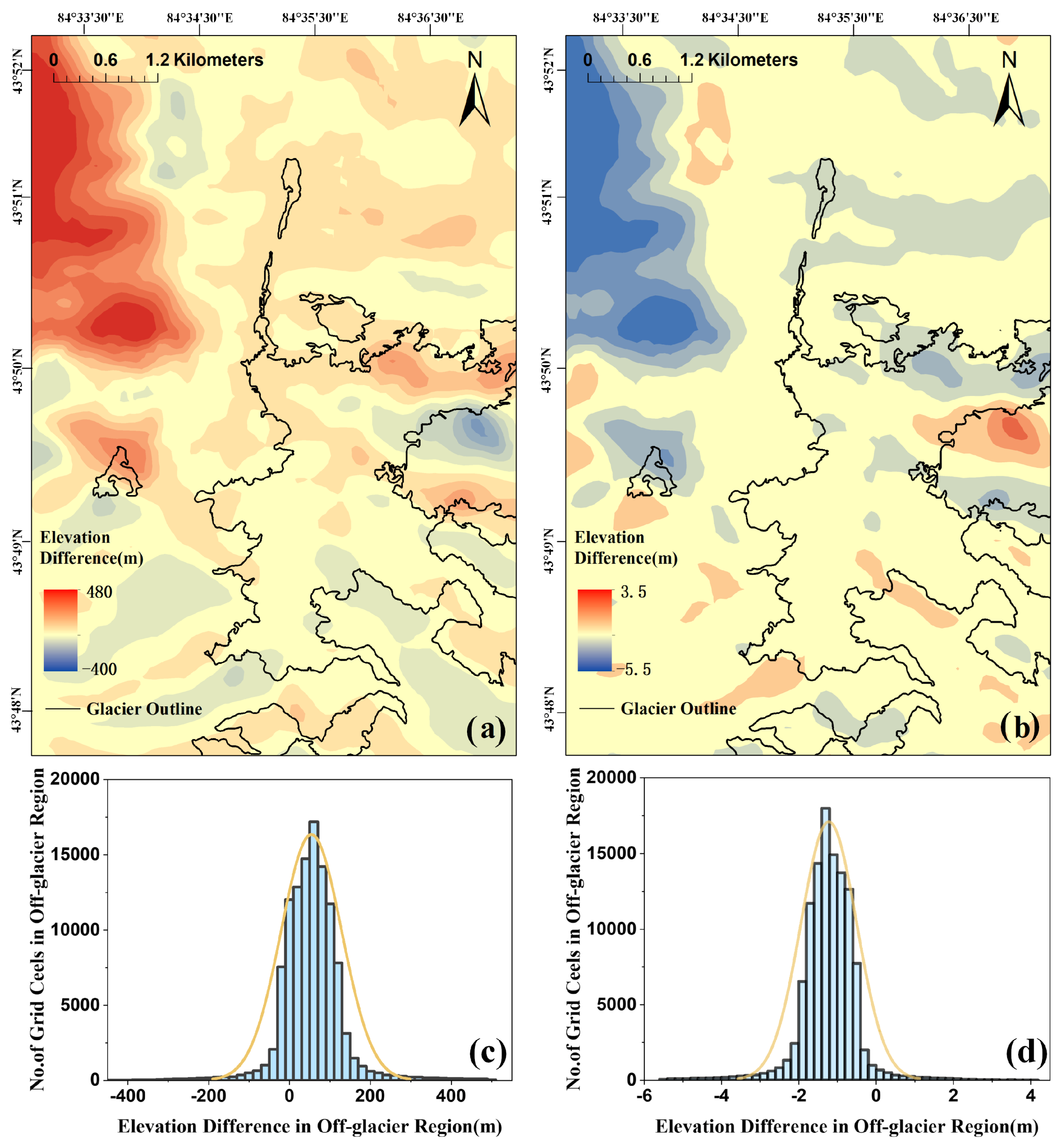
- Calculation of Elevation Changes from DEM DifferencingMeasured elevation changes have been used to investigate volume and mass changes in glacier for many studies. Accurate DEM differencing is key to calculate glacier elevation changes. Therefore, it is necessary to process the registration of the DEMs before calculating the glacier elevation changes. Due to the long wavelength of the C-band, there is an obvious penetration effect on the glacier, and the penetration depth is between 0∼10 m, especially in the glacier accumulation area [41]. Therefore, we preprocessed the SRTM DEM before DEM registration, as a result, the C-band SRTM DEM data corrected by the X-band SRTM DEM can represent the glacier surface height [30,42]. In this paper, the DEMs must be projected to the same map system, such as the universal transverse Mercator (UTM) system. In addition, because of the different spatial resolutions, one of the DEMs needs to be resampled to ensure the accuracy of the results. The abnormal values of surface elevation changes are altered through the Kriging interpolation algorithm. The elevation value we used now was proposed by McVicar, T.R. [43]. The method of processing the changes in elevation was taken from previous research work. The most frequently used DEM co-registration method, which is simple, analytic and robust was proposed by Nuth, C. and A. Kaab [44], and is based on the elevation derivative of slope and aspect and elevation difference residuals to correct the registration errors (Equation (1)).where is the elevation difference between the different DEMs, and are the terrain slope and aspect in the region, a is the magnitude elevation difference bias, b is the direction of the shift vector, c is the mean bias between the DEMs divided by the mean slope tangent of the terrain.Slope and aspect can be calculated by employing GIS. Previous research work has shown that the offset obtained by this method may not be the most suitable offset, and this process needs to be iterated to reach the optimal solution. In this paper, we iterate this process until the solution is solved. The process is terminated when the standard deviation is less than 2% to obtain the best registration result. The bias between DEMs is effectively eliminated through the use of fitting and solving to obtain the correction parameter pair after the DEM is registered. The result of DEM co-registration is illustrated in Figure 6. The glacier elevation changes were calculated based on the mean elevation difference between the DEM of two acquisition periods (2000–2015).
- (3)
- Calculation of Ablation VolumeCompared with the area of glaciers, we are more concerned about the changes in glacier volume. The volume of the ablation area is calculated by multiplying the area and elevation changes using an integral method. The combination of temporally consistent ablation area and elevation measurements is the crucial advantage of our method, which improves volume estimate accuracy. We improved the two-dimensional changes in the glacier to the three-dimensional changes in our study to obtain the susceptibility analysis of glacier debris flow based on glacier ablation.
2.2.4. Step 3: Susceptibility Analysis of Glacier Debris Flow
- (1)
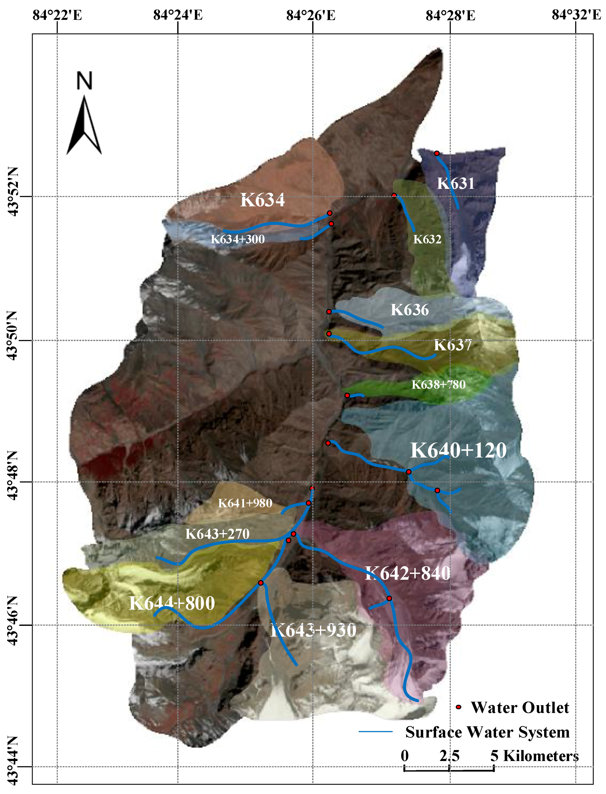
- The Divisions of Sub-watersheds in the Target AreaWe divided sub-watersheds in the target area considering hydrological statistics and an analysis module based on ASTER data. The main process is swale filling, traffic analysis, confluence accumulation statistics, water flow length calculation, river network extraction, etc. The result of watershed division is illustrated in Figure 7.
- (2)
- Brief Descriptions of the Geomorphic Information Entropy MethodGeomorphic condition is one of the three conditions necessary for the formation of debris flows, it is the background condition and potential energy condition of debris flows. The geomorphic information entropy method (GIE) of erosion watershed systems was proposed by Ai and Yue (1988) [47]. The GIE method depends on the area–elevation curve (Strahler) and combined the information entropy theory (Equation (2)). This theory has been validated to the evaluate of debris flows developed from traditional geomorphology. Some research work have been evaluated the susceptibility of debris flow based on the watershed erosion degree. For example, Wang, J. [47] used the geomorphic information method to evaluate the susceptibility in the strong earthquake area, Wenchuan. Li, Y.C. [48] used this method to obtain the susceptibility of each sub-basin in debris flow gullies.
3. Results
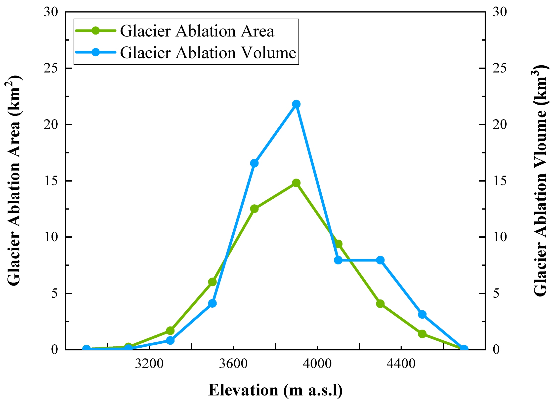
3.1. The Observation of Glacier Ablation and Recession
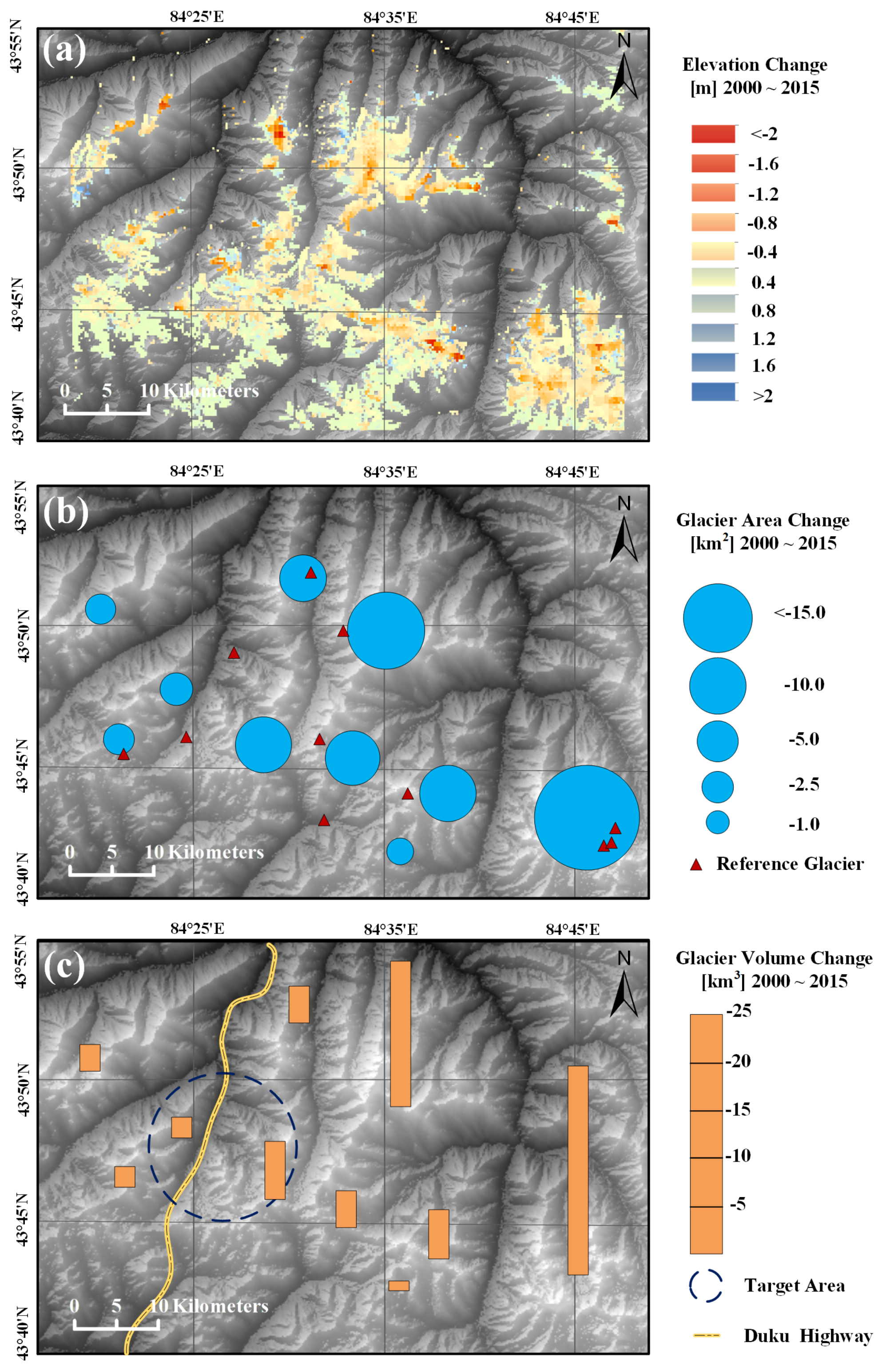
3.2. The Influence on the Glacier Shrinkage and Downwasting
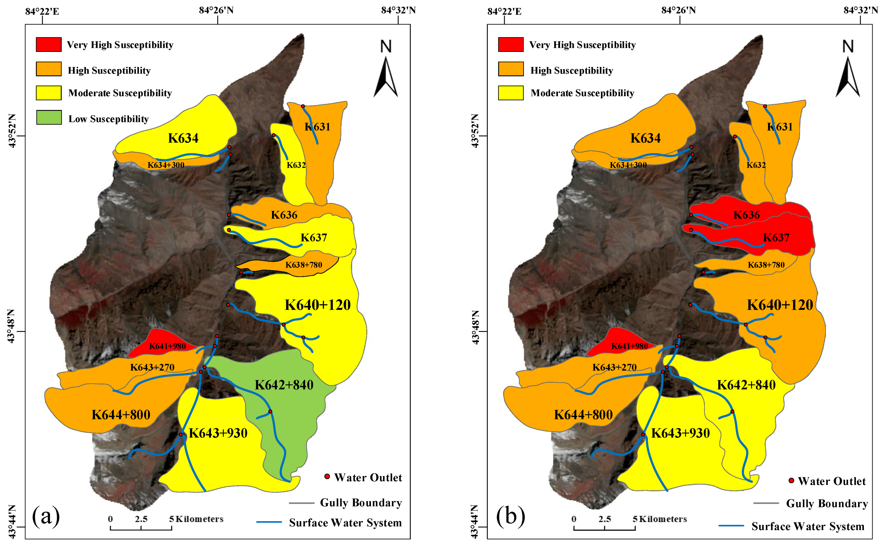
3.3. Susceptibility Analysis of Glacier Debris Flow
4. Discussion
5. Conclusions
Author Contributions
Funding
Institutional Review Board Statement
Informed Consent Statement
Data Availability Statement
Acknowledgments
Conflicts of Interest
Abbreviations
| DEM | Digital Elevation Model |
| ETM+ | The Enhanced Thematic Mapper Plus |
| GDEM | Global DEM |
| GIE | Geomorphic Information Entropy Method |
| GIS | Geographical Information System |
| GS | Gram-Schmidt |
| NDSI | Normalized Difference Snow Index |
| OLI | Operational Line Imager |
| TM | Thematic Mapper |
| UTM | Universal Transverse Mercator |
References
- Baggio, T.; Mergili, M.; D’Agostino, V. Advances in the simulation of debris flow erosion: The case study of the Rio Gere (Italy) event of the 4th August 2017. Geomorphology 2021, 381, 13. [Google Scholar] [CrossRef]
- Cenderelli, D.A.; Wohl, E.E. Peak discharge estimates of glacial-lake outburst floods and “normal” climatic floods in the Mount Everest region, Nepal. Geomorphology 2001, 40, 57–90. [Google Scholar] [CrossRef]
- Evans, S.G.; Roberts, N.J.; Ischuk, A.; Delaney, K.B.; Morozova, G.S.; Tutubalina, O. Landslides triggered by the 1949 Khait earthquake, Tajikistan, and associated loss of life. Eng. Geol. 2009, 109, 195–212. [Google Scholar] [CrossRef]
- Motschmann, A.; Huggel, C.; Carey, M.; Moulton, H.; Walker-Crawford, N.; Muñoz, R. Losses and damages connected to glacier retreat in the Cordillera Blanca, Peru. Clim. Change 2020, 162, 837–858. [Google Scholar] [CrossRef]
- Huggel, C.; Zgraggen-Oswald, S.; Haeberli, W.; Kääb, A.; Polkvoj, A.; Galushkin, I.; Evans, S.G. The 2002 rock/ice avalanche at Kolka/Karmadon, Russian Caucasus: Assessment of extraordinary avalanche formation and mobility, and application of QuickBird satellite imagery. Nat. Hazards Earth Syst. Sci. 2005, 5, 173–187. [Google Scholar] [CrossRef]
- Tang, W.; Ding, H.T.; Chen, N.S.; Ma, S.C.; Liu, L.H.; Wu, K.L.; Tian, S.F. Artificial Neural Network-based prediction of glacial debris flows in the Parlung Zangbo Basin, southeastern Tibetan Plateau, China. J. Mt. Sci. 2020, 18, 51–67. [Google Scholar] [CrossRef]
- Paul, F.; Bolch, T.; Kääb, A.; Nagler, T.; Nuth, C.; Scharrer, K.; Shepherd, A.; Strozzi, T.; Ticconi, F.; Bhambri, R.; et al. The glaciers climate change initiative: Methods for creating glacier area, elevation change and velocity products. Remote Sens. Environ. 2015, 162, 408–426. [Google Scholar] [CrossRef]
- Bayr, K.J.; Hall, D.K.; Kovalick, W.M. Observations on glaciers in the eastern Austrian Alps using satellite data. Int. J. Remote Sens. 1994, 15, 1733–1742. [Google Scholar] [CrossRef]
- Kulkarni, A.V. Glacial retreat in Himalaya using Indian remote sensing satellite data. In Agriculture and Hydrology Applications of Remote Sensing; Kuligowski, R.J., Parihar, J.S., Saito, G., Eds.; SPIE: Bellingham, WA, USA, 2006. [Google Scholar]
- Kääb, A.; Huggel, C.; Fischer, L.; Guex, S.; Paul, F.; Roer, I.; Salzmann, N.; Schlaefli, S.; Schmutz, K.; Schneider, D.; et al. Remote sensing of glacier- and permafrost-related hazards in high mountains: An overview. Nat. Hazards Earth Syst. Sci. 2005, 5, 527–554. [Google Scholar] [CrossRef]
- Elkadiri, R.; Sultan, M.; Youssef, A.M.; Elbayoumi, T.; Chase, R.; Bulkhi, A.B.; Al-Katheeri, M.M. A Remote Sensing-Based Approach for Debris-Flow Susceptibility Assessment Using Artificial Neural Networks and Logistic Regression Modeling. IEEE J. Sel. Top. Appl. Earth Observ. Remote Sens. 2014, 7, 4818–4835. [Google Scholar] [CrossRef]
- Cheng, Z.L.; Liu, J.J.; Liu, J.K. Debris flow induced by glacial lake break in southeast Tibet. In Montoring, Simulation, Prevention and Remediation of Dense Debris Flows Iii; DeWrachien, D., Brebbia, C.A., Eds.; Wit Press: Southampton, UK, 2010; pp. 101–111. [Google Scholar]
- Deng, M.; Chen, N.; Liu, M. Meteorological factors driving glacial till variation and the associated periglacial debris flows in Tianmo Valley, south-eastern Tibetan Plateau. Nat. Hazards Earth Syst. Sci. 2017, 17, 345–356. [Google Scholar] [CrossRef]
- Golovko, D.; Roessner, S.; Behling, R.; Wetzel, H.U.; Kleinschmit, B. Evaluation of Remote-Sensing-Based Landslide Inventories for Hazard Assessment in Southern Kyrgyzstan. Remote Sens. 2017, 9, 943. [Google Scholar] [CrossRef]
- Cannon, S.H.; Boldt, E.M.; Laber, J.L.; Kean, J.W.; Staley, D.M. Rainfall intensity-duration thresholds for postfire debris-flow emergency-response planning. Nat. Hazards 2011, 59, 209–236. [Google Scholar] [CrossRef]
- Chen, N.; Yang, C.; Zhou, W.; Hu, G.; Li, H.; Hand, D. The Critical Rainfall Characteristics for Torrents and Debris Flows in the Wenchuan Earthquake Stricken Area (vol 6, pg 362, 2009). J. Mt. Sci. 2010, 7, A1. [Google Scholar] [CrossRef]
- Rickenmann, D. Empirical relationships for debris flows. Nat. Hazards 1999, 19, 47–77. [Google Scholar] [CrossRef]
- Allen, S.K.; Rastner, P.; Arora, M.; Huggel, C.; Stoffel, M. Lake outburst and debris flow disaster at Kedarnath, June 2013: Hydrometeorological triggering and topographic predisposition. Landslides 2016, 13, 1479–1491. [Google Scholar] [CrossRef]
- Chang, M.; Dou, X.; Hales, T.C.; Yu, B. Patterns of rainfall-threshold for debris-flow occurrence in the Wenchuan seismic region, Southwest China. Bull. Eng. Geol. Environ. 2021, 80, 2117–2130. [Google Scholar] [CrossRef]
- Xiaojun, G.; Peng, C.; Xingchang, C.; Yong, L.; Ju, Z.; Yuqing, S. Spatial uncertainty of rainfall and its impact on hydrological hazard forecasting in a small semiarid mountainous watershed. J. Hydrol. 2021, 595, 126049. [Google Scholar] [CrossRef]
- Huebl, J.; Kaitna, R. Monitoring Debris-Flow Surges and Triggering Rainfall at the Lattenbach Creek, Austria. Environ. Eng. Geosci. 2021, 27, 213–220. [Google Scholar] [CrossRef]
- Kumar, A.; Bhambri, R.; Tiwari, S.K.; Verma, A.; Gupta, A.K.; Kawishwar, P. Evolution of debris flow and moraine failure in the Gangotri Glacier region, Garhwal Himalaya: Hydro-geomorphological aspects. Geomorphology 2019, 333, 152–166. [Google Scholar] [CrossRef]
- Chiarle, M.; Iannotti, S.; Mortara, G.; Deline, P. Recent debris flow occurrences associated with glaciers in the Alps. Glob. Planet. Change 2007, 56, 123–136. [Google Scholar] [CrossRef]
- Beniston, M. Climatic change in mountain regions: A review of possible impacts. Clim. Change 2003, 59, 5–31. [Google Scholar] [CrossRef]
- Alean, J. Ice avalanches—Some empirical information about their formation and reach. J. Glaciol. 1985, 31, 324–333. [Google Scholar] [CrossRef]
- Quincey, D.J.; Richardson, S.D.; Luckman, A.; Lucas, R.M.; Reynolds, J.M.; Hambrey, M.J.; Glasser, N.F. Early recognition of glacial lake hazards in the Himalaya using remote sensing datasets. Glob. Planet. Change 2007, 56, 137–152. [Google Scholar] [CrossRef]
- Andreassen, L.M.; Paul, F.; Kääb, A.; Hausberg, J.E. Landsat-derived glacier inventory for Jotunheimen, Landsat-derived glacier inventory for Jotunheimen, Norway, and deduced glacier changes since the 1930s. Cryosphere 2008, 2, 131–145. [Google Scholar] [CrossRef]
- Dozier, J. Spectral signature of alpine snow cover from the landsat thematic mapper. Remote Sens. Environ. 1989, 28, 9–22. [Google Scholar] [CrossRef]
- Frey, H.; Paul, F.; Strozzi, T. Compilation of a glacier inventory for the western Himalayas from satellite data: Methods, challenges, and results. Remote Sens. Environ. 2012, 124, 832–843. [Google Scholar] [CrossRef]
- Gardelle, J.; Berthier, E.; Arnaud, Y. Impact of resolution and radar penetration on glacier elevation changes computed from DEM differencing. J. Glaciol. 2012, 58, 419–422. [Google Scholar] [CrossRef]
- Aniya, M.; Sato, H.; Naruse, R.; Skvarca, P.; Casassa, G. The use of satellite and airborne imagery to inventory outlet glaciers of the Southern Patagonia Icefield, South America. Photogram. Eng. Remote Sens. 1996, 62, 1361–1369. [Google Scholar]
- Gjermundsen, E.F.; Mathieu, R.; Kääb, A.; Chinn, T.; Fitzharris, B.; Hagen, J.O. Assessment of multispectral glacier mapping methods and derivation of glacier area changes, 1978–2002, in the central Southern Alps, New Zealand, from ASTER satellite data, field survey and existing inventory data. J. Glaciol. 2017, 57, 667–683. [Google Scholar] [CrossRef]
- Le Bris, R.; Paul, F.; Frey, H.; Bolch, T. A new satellite-derived glacier inventory for western Alaska. Ann. Glaciol. 2017, 52, 135–143. [Google Scholar] [CrossRef]
- Kumar, M.; Al-Quraishi, A.M.F.; Mondal, I. Glacier changes monitoring in Bhutan High Himalaya using remote sensing technology. Environ. Eng. Res. 2021, 26, 8. [Google Scholar] [CrossRef]
- Bolch, T.; Buchroithner, M.; Pieczonka, T.; Kunert, A. Planimetric and volumetric glacier changes in the Khumbu Himal, Nepal, since 1962 using Corona, Landsat TM and ASTER data. J. Glaciol. 2008, 54, 592–600. [Google Scholar] [CrossRef]
- Tong, R.; Parajka, J.; Komma, J.; Blöschl, G. Mapping snow cover from daily Collection 6 MODIS products over Austria. J. Hydrol. 2020, 590, 10. [Google Scholar] [CrossRef]
- Yan, L.; Wang, J.; Hao, X.; Tang, Z. Glacier mapping based on rough set theory in the Manas River watershed. Adv. Space Res. 2014, 53, 1071–1080. [Google Scholar] [CrossRef]
- Li, Z.; Shi, X.; Tang, Q.; Zhang, Y.; Gao, H.; Pan, X.; Déry, S.J.; Zhou, P. Partitioning the contributions of glacier melt and precipitation to the 1971–2010 runoff increases in a headwater basin of the Tarim River. J. Hydrol. 2020, 583, 10. [Google Scholar] [CrossRef]
- Bolch, T.; Peters, J.; Yegorov, A.; Pradhan, B.; Buchroithner, M.; Blagoveshchensky, V. Identification of potentially dangerous glacial lakes in the northern Tien Shan. Nat. Hazards 2011, 59, 1691–1714. [Google Scholar] [CrossRef]
- Falatkova, K.; Šobr, M.; Neureiter, A.; Schöner, W.; Janský, B.; Häusler, H.; Engel, Z.; Beneš, V. Development of proglacial lakes and evaluation of related outburst susceptibility at the Adygine ice-debris complex, northern Tien Shan. Earth Surf. Dyn. 2019, 7, 301–320. [Google Scholar] [CrossRef]
- Barandun, M.; Huss, M.; Sold, L.; Farinotti, D.; Azisov, E.; Salzmann, N.; Usubaliev, R.; Merkushkin, A.; Hoelzle, M. Re-analysis of seasonal mass balance at Abramov glacier 1968–2014. J. Glaciol. 2015, 61, 1103–1117. [Google Scholar] [CrossRef]
- Larsen, C.F.; Motyka, R.J.; Arendt, A.A.; Echelmeyer, K.A.; Geissler, P.E. Glacier changes in southeast Alaska and northwest British Columbia and contribution to sea level rise. J. Geophys. Res. Earth Surf. 2007, 112, 11. [Google Scholar] [CrossRef]
- McVicar, T.R.; Körner, C. On the use of elevation, altitude, and height in the ecological and climatological literature. Oecologia 2013, 171, 335–337. [Google Scholar] [CrossRef]
- Nuth, C.; Kaab, A. Co-registration and bias corrections of satellite elevation data sets for quantifying glacier thickness change. Cryosphere 2011, 5, 271–290. [Google Scholar] [CrossRef]
- Huggel, C.; Haeberli, W.; Kääb, A.; Bieri, D.; Richardson, S. An assessment procedure for glacial hazards in the Swiss Alps. Can. Geotech. J. 2004, 41, 1068–1083. [Google Scholar] [CrossRef]
- Zaginaev, V.; Petrakov, D.; Erokhin, S.; Meleshko, A.; Stoffel, M.; Ballesteros-Cánovas, J.A. Geomorphic control on regional glacier lake outburst flood and debris flow activity over northern Tien Shan. Glob. Planet. Change 2019, 176, 50–59. [Google Scholar] [CrossRef]
- Wang, J.; Yu, Y.; Yang, S.; Lu, G.H.; Ou, G.Q. A modified certainty coefficient method (M-CF) for debris flow susceptibility assessment: A case study for the Wenchuan earthquake meizoseismal areas. J. Mt. Sci. 2014, 11, 1286–1297. [Google Scholar] [CrossRef]
- Li, Y.; Chen, J.; Zhang, Y.; Song, S.; Han, X.; Ammar, M. Debris Flow Susceptibility Assessment and Runout Prediction: A Case Study in Shiyang Gully, Beijing, China. Int. J. Environ. Res. 2020, 14, 365–383. [Google Scholar] [CrossRef]
- Schiefer, E.; Menounos, B.; Wheate, R. Recent volume loss of British Columbian glaciers, Canada. Geophys. Res. Lett. 2007, 34, 6. [Google Scholar] [CrossRef]
- Tak, S.; Keshari, A.K. Investigating mass balance of Parvati glacier in Himalaya using satellite imagery based model. Sci. Rep. 2020, 10, 16. [Google Scholar] [CrossRef]
- Sommer, C.; Malz, P.; Seehaus, T.C.; Lippl, S.; Zemp, M.; Braun, M.H. Rapid glacier retreat and downwasting throughout the European Alps in the early 21(st) century. Nat. Commun. 2020, 11, 10. [Google Scholar] [CrossRef]
- Romshoo, S.A.; Fayaz, M.; Meraj, G.; Bahuguna, I.M. Satellite-observed glacier recession in the Kashmir Himalaya, India, from 1980 to 2018. Environ. Monit. Assess. 2020, 192, 17. [Google Scholar] [CrossRef]
- Fujita, K.; Nuimura, T. Spatially heterogeneous wastage of Himalayan glaciers. Proc. Natl. Acad. Sci. USA 2011, 108, 14011–14014. [Google Scholar] [CrossRef] [PubMed]
- Wang, W.; Xiang, Y.; Gao, Y.; Lu, A.; Yao, T. Rapid expansion of glacial lakes caused by climate and glacier retreat in the Central Himalayas. Hydrol. Process. 2015, 29, 859–874. [Google Scholar] [CrossRef]
- Das, S.; Sharma, M.C. Glacier changes between 1971 and 2016 in the Jankar Chhu Watershed, Lahaul Himalaya, India. J. Glaciol. 2019, 65, 13–28. [Google Scholar] [CrossRef]


| Sensor Type | Acquisition Date | Images Resolution (m) | Snow-Covered | Applicability |
|---|---|---|---|---|
| Landsat TM | 08/07/2000 | 30 | Seasonal snow | Glacier boundaries/Glacier surface elevation |
| 04/13/2013 | Glacier boundaries | |||
| Landsat OLI | 06/13/2015 | 30 | Snow free | Glacier boundaries/Glacier surface elevation |
| 05/09/2020 | Glacier boundaries |
| Data Type | Images Resolution (m) | Acquisition Type | Time Period |
|---|---|---|---|
| SRTM | 90 | Radar interferometry | February, 2000 |
| ASTER | 30 | Optical photogrammetry | 2000–present |
| TanDEM-X | 12 | Radar interferometry | 2010–present |
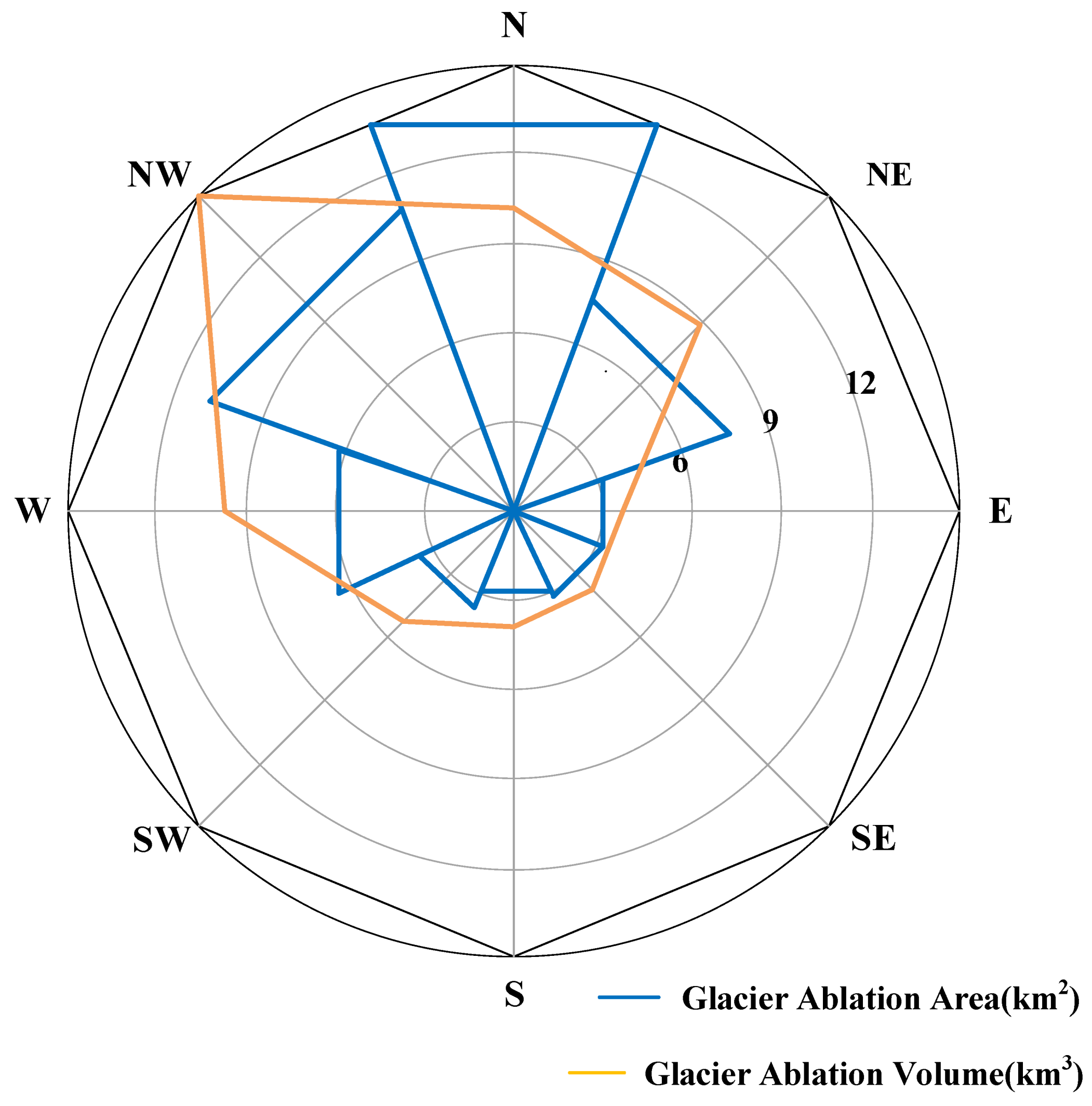
| Aspect | Range () | Glacier Ablation Area (km) | Glacier Ablation Volume (km) |
|---|---|---|---|
| N | 0∼22.5 (337.5∼360) | 13.7 | 10.0 |
| NE | 22.5∼112.5 | 7.20 | 8.9 |
| E | 67.5∼112.5 | 3.0 | 3.8 |
| SE | 112.5∼157.5 | 3.2 | 4.0 |
| S | 157.5∼202.5 | 2.9 | 4.4 |
| SW | 202.5∼247.5 | 3.8 | 5.6 |
| W | 247.5∼292.5 | 5.8 | 9.4 |
| NW | 292.5∼337.5 | 10.2 | 15.7 |
| Basin Number | Maximum Elevation Difference (m) | Basin Area (km) | Glacier Area (km) | Glacier Coverage Rate | Glacier Ablation Area (km) | Mean Elevation Variation (m) | Glacier Ablation Volume (km) |
|---|---|---|---|---|---|---|---|
| K631 | 2350 | 5.03 | 0.26 | 0.05 | 0.25 | −1.82 | 0.46 |
| K632 | 2224 | 3.16 | 0.09 | 0.02 | 0.01 | −2.46 | 0.03 |
| K636 | 2255 | 3.68 | 0.13 | 0.04 | 0.24 | −3.95 | 0.99 |
| K637 | 2205 | 4.82 | 0.06 | 0.01 | 0.59 | −2.72 | 1.62 |
| K638+780 | 1817 | 2.22 | 0.24 | 0.1 | 0.18 | −2.27 | 0.39 |
| K640+120 | 2190 | 13.29 | 0.39 | 0.03 | 0.70 | −0.93 | 0.61 |
| K642+840 | 1813 | 12.454 | 1.3 | 0.1 | 0.69 | −1.60 | 1.10 |
| K643+930 | 1624 | 12.21 | 2.47 | 0.2 | 0.42 | −1.75 | 0.71 |
| K634 | 2042 | 6.29 | 0 | 0 | 0.069 | −3.05 | 0.22 |
| K634+300 | 1491 | 1.93 | 0 | 0 | 0.16 | −3.80 | 0.62 |
| K641+980 | 1473 | 1.59 | 0.007 | 0.004 | 0.03 | −3.28 | 0.09 |
| K643+270 | 1961 | 4.72 | 0.14 | 0.03 | 0.15 | −2.02 | 0.29 |
| K644+800 | 1874 | 8.33 | 0.99 | 0.12 | 0.28 | −1.14 | 0.30 |
| Basin Number | H | Glacier Coverage Rate | Hg | Development | Assessment |
|---|---|---|---|---|---|
| K631 | 0.19 | 0.05 | 0.1805 | Mature but bias infancy | H |
| K632 | 0.21 | 0.02 | 0.2058 | Mature | M |
| K636 | 0.16 | 0.04 | 0.1536 | Mature but bias infancy | H |
| K637 | 0.24 | 0.01 | 0.2376 | Mature | M |
| K638+780 | 0.21 | 0.1 | 0.189 | Mature but bias infancy | H |
| K640+120 | 0.21 | 0.03 | 0.2037 | Mature | M |
| K642+840 | 0.37 | 0.1 | 0.333 | Mature but bias old stage | L |
| K643+930 | 0.37 | 0.2 | 0.296 | Mature | M |
| K634 | 0.21 | 0 | 0.21 | Mature | M |
| K634+300 | 0.19 | 0 | 0.19 | Mature but bias infancy | H |
| K641+980 | 0.09 | 0.004 | 0.0896 | Infancy | VH |
| K643+270 | 0.19 | 0.03 | 0.1843 | Mature but bias infancy | H |
| K644+800 | 0.20 | 0.12 | 0.176 | Mature but bias infancy | H |
| Basin Number | H | Correction Factor | Hg | Development | Assessment |
|---|---|---|---|---|---|
| K631 | 0.19 | 0.85 | 0.1615 | Mature but bias infancy | H |
| K632 | 0.21 | 0.95 | 0.1995 | Mature but bias infancy | H |
| K636 | 0.16 | 0.65 | 0.104 | Infancy | VH |
| K637 | 0.24 | 0.45 | 0.108 | Infancy | VH |
| K638+780 | 0.21 | 0.85 | 0.1785 | Mature but bias infancy | H |
| K640+120 | 0.21 | 0.75 | 0.1575 | Mature but bias infancy | H |
| K642+840 | 0.37 | 0.6 | 0.222 | Mature | M |
| K643+930 | 0.37 | 0.8 | 0.296 | Mature | M |
| K634 | 0.21 | 0.9 | 0.189 | Mature but bias infancy | H |
| K634+300 | 0.19 | 0.75 | 0.1425 | Mature but bias infancy | H |
| K641+980 | 0.09 | 0.95 | 0.0855 | Infancy | VH |
| K643+270 | 0.19 | 0.9 | 0.171 | Mature but bias infancy | H |
| K644+800 | 0.20 | 0.9 | 0.18 | Mature but bias infancy | H |
| Number | Distribution | Type | Scale | Assessment |
|---|---|---|---|---|
| N1 | K631 | Valley pattern | Large | H |
| N2 | K632 | Valley pattern | Small | H |
| N3 | K634 | Valley pattern | Medium | H |
| N4 | K634+300 | Valley pattern | Small | H |
| N5 | K636 | Valley pattern | Large | VH |
| N6 | K637 | Valley pattern | Medium | VH |
| N7 | K638+780 | Valley pattern | Small | H |
| N8 | K640+120 | Valley pattern | Medium | H |
| N9 | K641+980 | Valley pattern | Small | VH |
| N10 | K642+840 | Valley pattern | Small | M |
| N11 | K643+270 | Valley pattern | Small | H |
| N12 | K643+930 | Valley pattern | Small | M |
| N13 | K644+800 | Valley pattern | Small | H |
Publisher’s Note: MDPI stays neutral with regard to jurisdictional claims in published maps and institutional affiliations. |
© 2021 by the authors. Licensee MDPI, Basel, Switzerland. This article is an open access article distributed under the terms and conditions of the Creative Commons Attribution (CC BY) license (https://creativecommons.org/licenses/by/4.0/).
Share and Cite
Lin, R.; Mei, G.; Liu, Z.; Xi, N.; Zhang, X. Susceptibility Analysis of Glacier Debris Flow by Investigating the Changes in Glaciers Based on Remote Sensing: A Case Study. Sustainability 2021, 13, 7196. https://doi.org/10.3390/su13137196
Lin R, Mei G, Liu Z, Xi N, Zhang X. Susceptibility Analysis of Glacier Debris Flow by Investigating the Changes in Glaciers Based on Remote Sensing: A Case Study. Sustainability. 2021; 13(13):7196. https://doi.org/10.3390/su13137196
Chicago/Turabian StyleLin, Ruoshen, Gang Mei, Ziyang Liu, Ning Xi, and Xiaona Zhang. 2021. "Susceptibility Analysis of Glacier Debris Flow by Investigating the Changes in Glaciers Based on Remote Sensing: A Case Study" Sustainability 13, no. 13: 7196. https://doi.org/10.3390/su13137196
APA StyleLin, R., Mei, G., Liu, Z., Xi, N., & Zhang, X. (2021). Susceptibility Analysis of Glacier Debris Flow by Investigating the Changes in Glaciers Based on Remote Sensing: A Case Study. Sustainability, 13(13), 7196. https://doi.org/10.3390/su13137196