
Performance Evaluation of Five GIS-Based Models for Landslide Susceptibility Prediction and Mapping: A Case Study of Kaiyang County, China


Abstract
1. Introduction
2. Materials and Methods
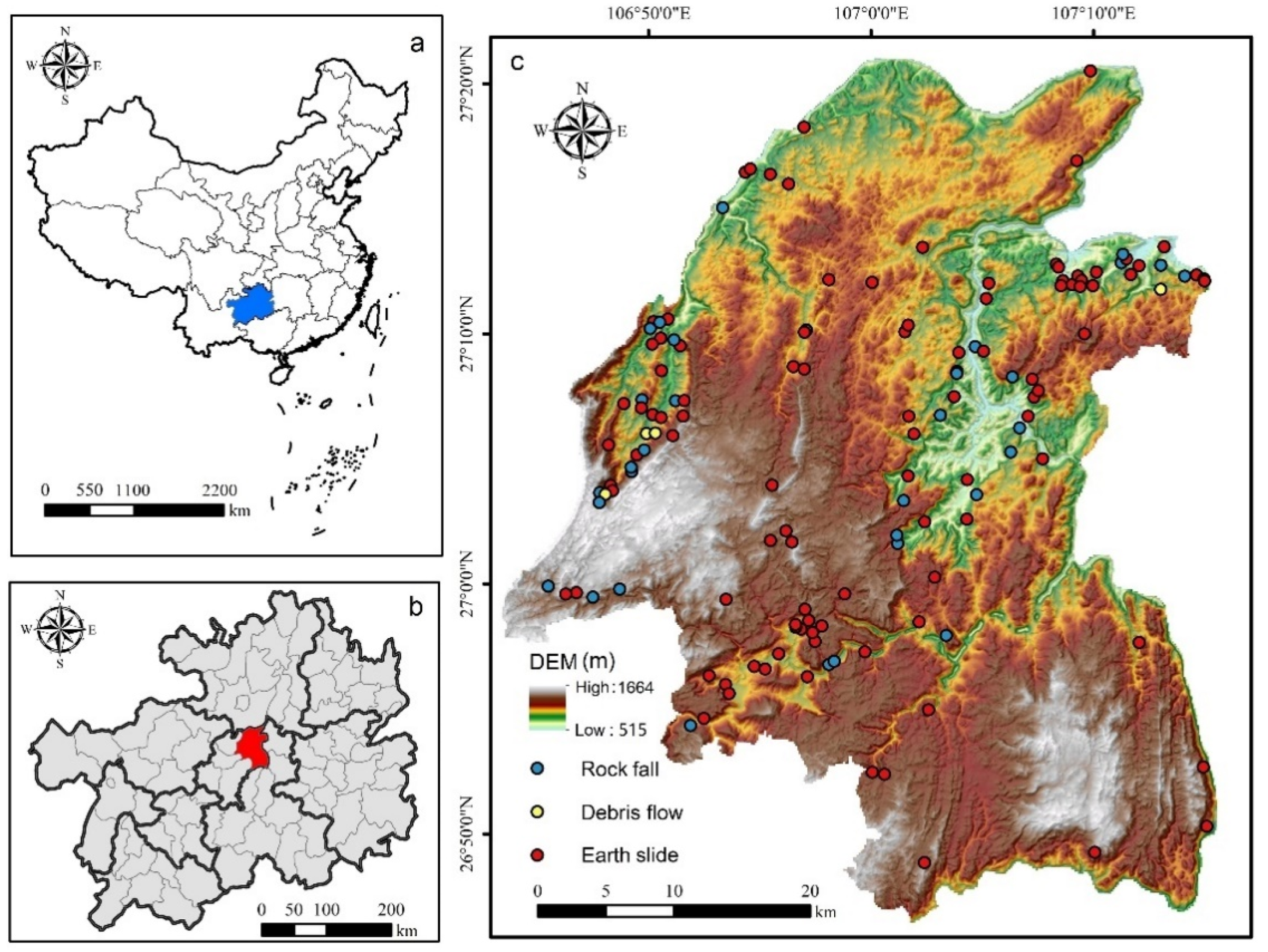
2.1. Study Area
2.2. Methodology
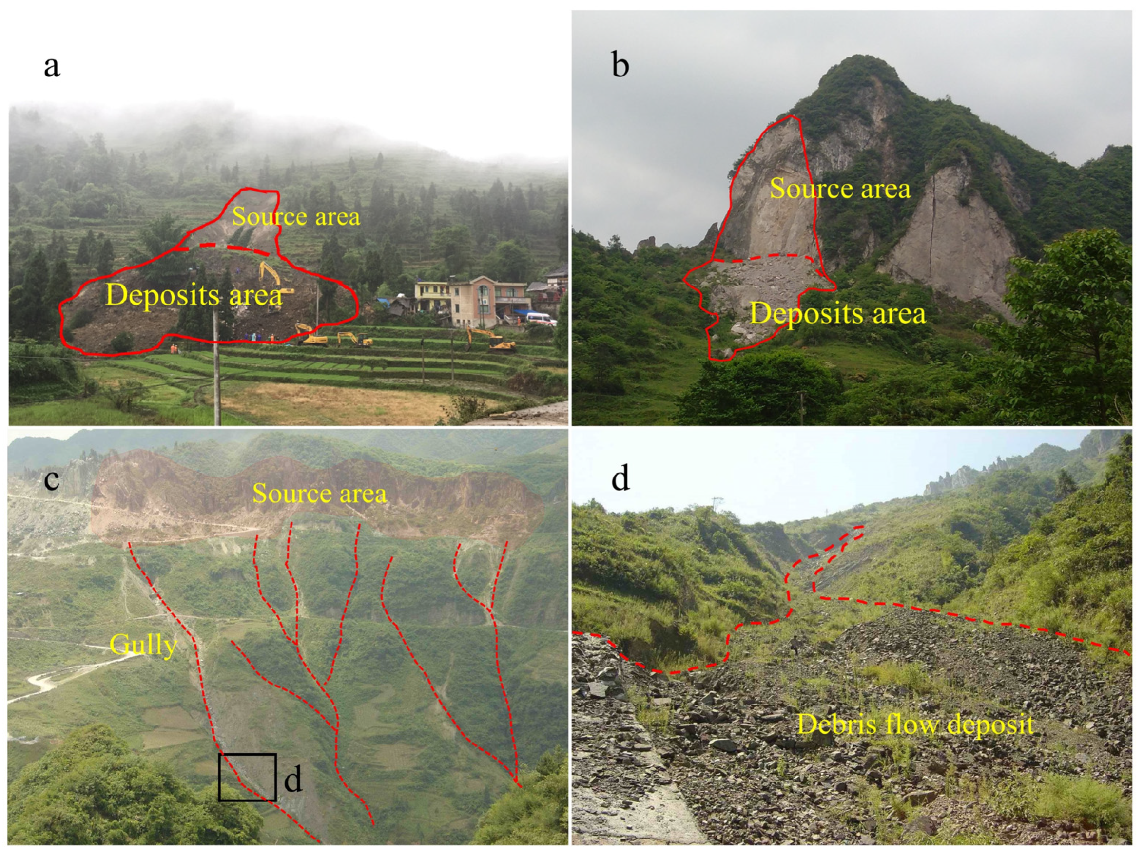
2.3. Landslide Inventory Map
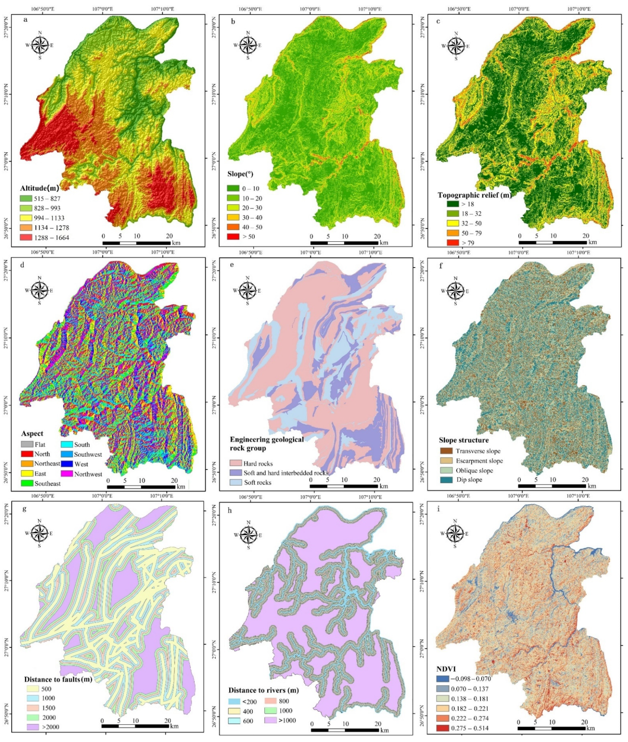
Landslide Conditioning Factors
2.4. Correlations between Landslides and Their Conditioning Factors
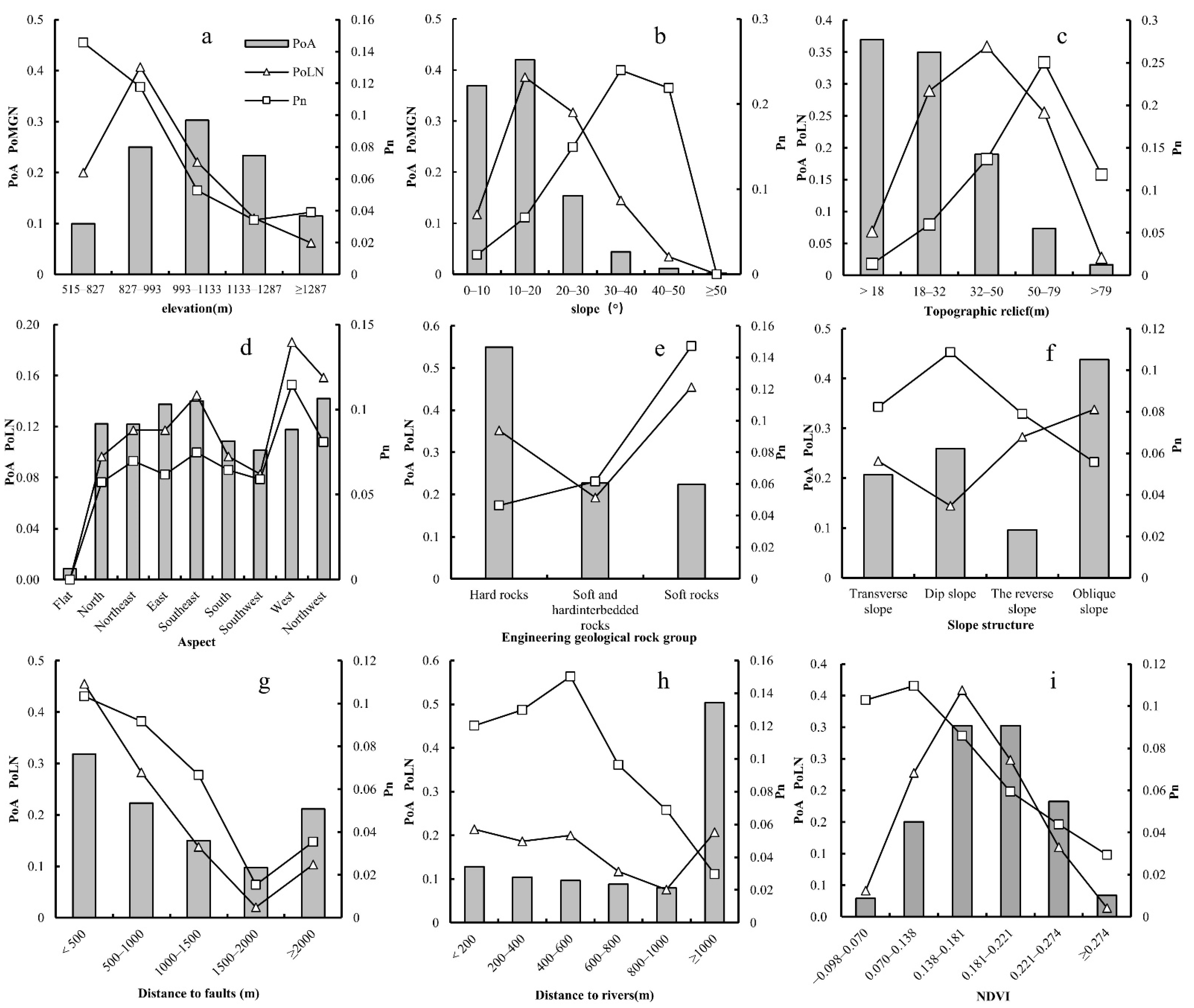
2.4.1. Altitude
2.4.2. Slope
2.4.3. Topographic Relief
2.4.4. Aspect
2.4.5. Engineering Geological Rock Group
2.4.6. Slope Structure
2.4.7. Distance to Faults
2.4.8. Distance to Rivers
2.4.9. Normalized Difference Vegetation Index (NDVI)
2.5. Correlations Analysis of Landslide Conditioning Factors
2.6. Susceptibility Mapping Models
2.6.1. Certainty Factor (CF) Model
2.6.2. Analytic Hierarchy Process (AHP)
2.6.3. Logistic Regression (LR) Model
2.6.4. CF-AHP Integrated Model
2.6.5. CF-LR Integrated Model
3. Results and Discussion
3.1. Certainty Factor (CF) Model
3.2. AHP
3.3. LR Model
3.4. CF-AHP Integrated Model
3.5. CF-LR Integrated Model
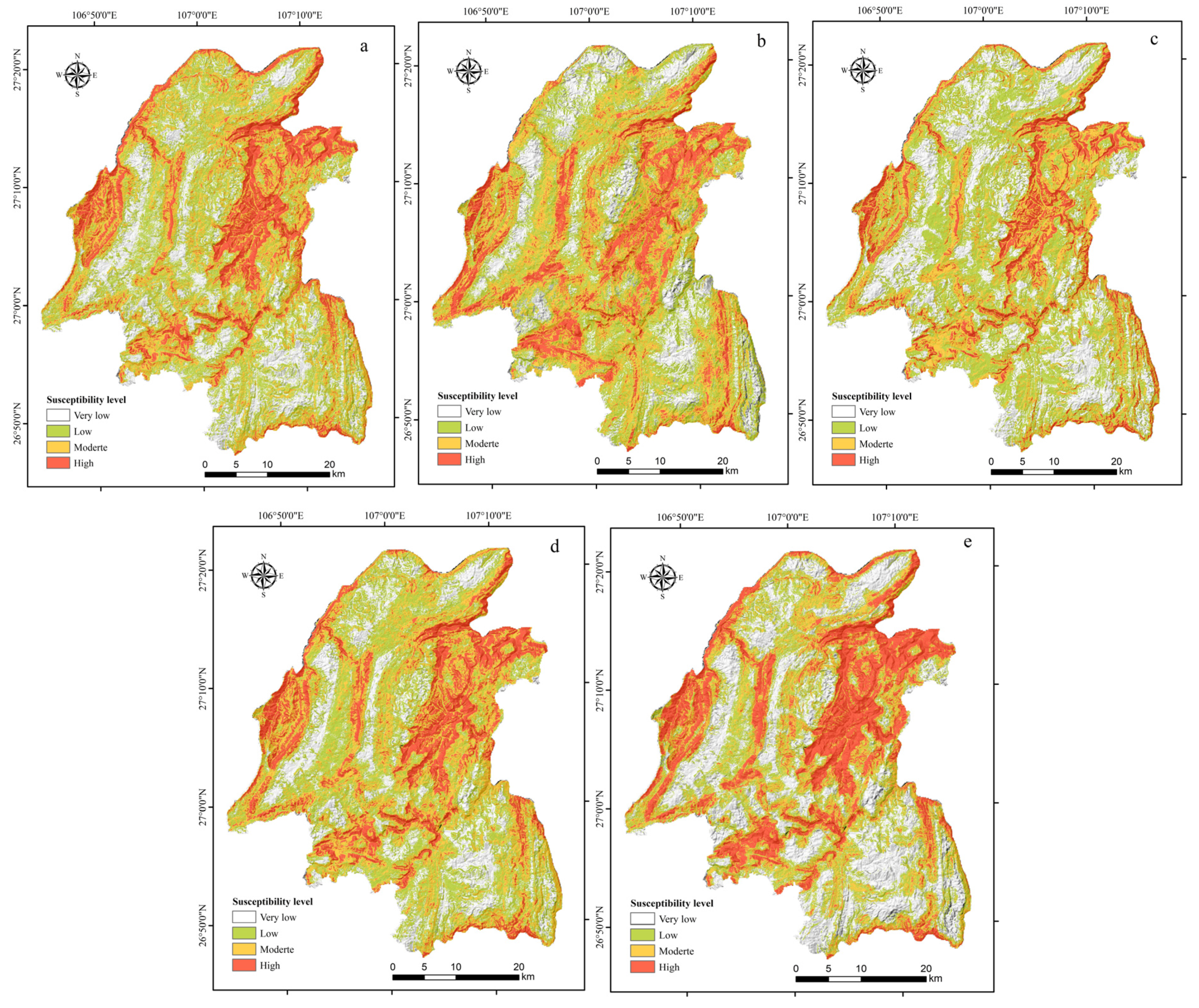
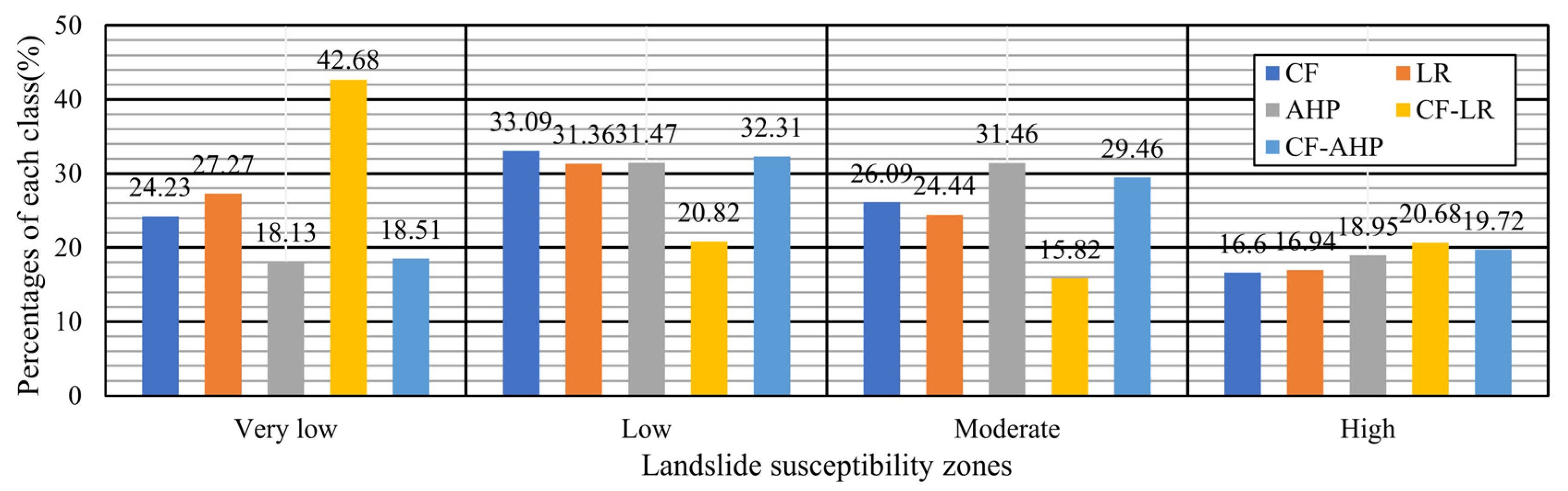
3.6. Landslide Susceptibility Mapping
3.7. Validation of the Susceptibility Models
3.7.1. Distribution of Landslides
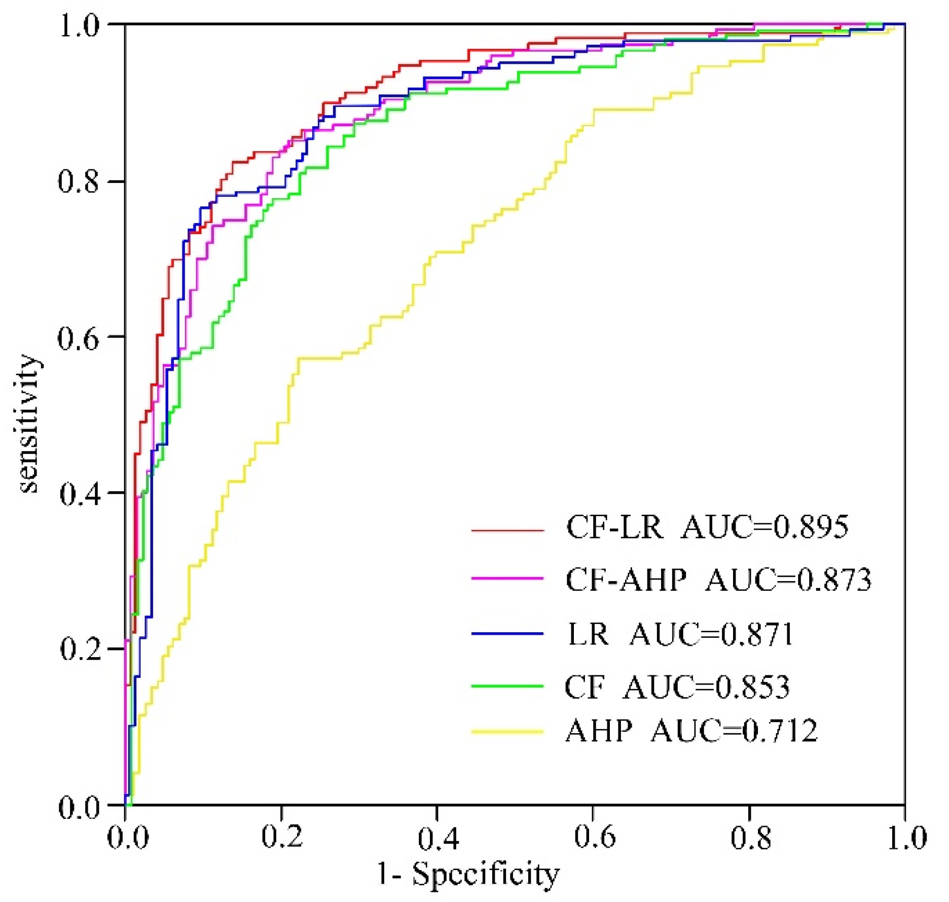
3.7.2. Receiver Operating Characteristic Curves
3.8. Uncertainty Analysis
4. Conclusions
Author Contributions
Funding
Institutional Review Board Statement
Informed Consent Statement
Acknowledgments
Conflicts of Interest
References
- Varnes, D.J. Landslide hazard zonation: A review of principles and practice. Nat. Hazards 1984, 3, 63. [Google Scholar] [CrossRef]
- Jeong, S.; Kassim, A.; Hong, M.; Saadatkhah, N. Susceptibility Assessments of Landslides in Hulu Kelang Area Using a Geographic Information System-Based Prediction Model. Sustainability 2018, 10, 2941. [Google Scholar] [CrossRef]
- Nguyen, V.-T.; Tran, T.H.; Ha, N.A.; Ngo, V.L.; Nadhir, A.-A.; Tran, V.P.; Duy Nguyen, H.; Ma, M.; Amini, A.; Prakash, I.; et al. GIS Based Novel Hybrid Computational Intelligence Models for Mapping Landslide Susceptibility: A Case Study at Da Lat City, Vietnam. Sustainability 2019, 11, 7118. [Google Scholar] [CrossRef]
- Harrison, J.F.; Chang, C.-H. Sustainable Management of a Mountain Community Vulnerable to Geohazards: A Case Study of Maolin District, Taiwan. Sustainability 2019, 11, 4107. [Google Scholar] [CrossRef]
- Lin, G.-W.; Chen, H.; Shih, T.-Y.; Lin, S. Various links between landslide debris and sediment flux during earthquake and rainstorm events. J. Asian Earth Sci. 2012, 54–55, 41–48. [Google Scholar] [CrossRef]
- Ma, T.; Li, C.; Lu, Z.; Bao, Q. Rainfall intensity–duration thresholds for the initiation of landslides in Zhejiang Province, China. Geomorphology 2015, 245, 193–206. [Google Scholar] [CrossRef]
- Wang, L.-J.; Guo, M.; Sawada, K.; Lin, J.; Zhang, J. Landslide susceptibility mapping in Mizunami City, Japan: A comparison between logistic regression, bivariate statistical analysis and multivariate adaptive regression spline models. Catena 2015, 135, 271–282. [Google Scholar] [CrossRef]
- Xu, C.; Xu, X.; Shyu, J.B.H.; Zheng, W.; Min, W. Landslides triggered by the 22 July 2013 Minxian–Zhangxian, China, Mw 5.9 earthquake: Inventory compiling and spatial distribution analysis. J. Asian Earth Sci. 2014, 92, 125–142. [Google Scholar] [CrossRef]
- Fell, R.; Corominas, J.; Bonnard, C.; Cascini, L.; Leroi, E.; Savage, W.Z. Guidelines for landslide susceptibility, hazard and risk zoning for land use planning. Eng. Geol. 2008, 102, 85–98. [Google Scholar] [CrossRef]
- Saha, A.K.; Gupta, R.P.; Sarkar, I.; Arora, M.K.; Csaplovics, E. An approach for GIS-based statistical landslide susceptibility zonation?with a case study in the Himalayas. Landslides 2005, 2, 61–69. [Google Scholar] [CrossRef]
- Trigila, A.; Iadanza, C.; Esposito, C.; Scarascia-Mugnozza, G. Comparison of Logistic Regression and Random Forests techniques for shallow landslide susceptibility assessment in Giampilieri (NE Sicily, Italy). Geomorphology 2015, 249, 119–136. [Google Scholar] [CrossRef]
- Jiang, W.; Rao, P.; Cao, R.; Tang, Z.; Chen, K. Comparative evaluation of geological disaster susceptibility using multi-regression methods and spatial accuracy validation. J. Geogr. Sci. 2017, 27, 439–462. [Google Scholar] [CrossRef]
- Champati ray, P.K.; Dimri, S.; Lakhera, R.C.; Sati, S. Fuzzy-based method for landslide hazard assessment in active seismic zone of Himalaya. Landslides 2006, 4, 101–111. [Google Scholar] [CrossRef]
- Kanungo, D.P.; Arora, M.K.; Gupta, R.P.; Sarkar, S. Landslide risk assessment using concepts of danger pixels and fuzzy set theory in Darjeeling Himalayas. Landslides 2008, 5, 407–416. [Google Scholar] [CrossRef]
- Pradhan, B. Application of an advanced fuzzy logic model for landslide susceptibility analysis. Int. J. Comput. Intell. Syst. 2010, 3, 370–381. [Google Scholar] [CrossRef]
- Chen, W.; Li, W.; Chai, H.; Hou, E.; Li, X.; Ding, X. GIS-based landslide susceptibility mapping using analytical hierarchy process (AHP) and certainty factor (CF) models for the Baozhong region of Baoji City, China. Environ. Earth Sci. 2015, 75, 63. [Google Scholar] [CrossRef]
- Demir, G.; Aytekin, M.; Akgün, A.; İkizler, S.B.; Tatar, O. A comparison of landslide susceptibility mapping of the eastern part of the North Anatolian Fault Zone (Turkey) by likelihood-frequency ratio and analytic hierarchy process methods. Nat. Hazards 2013, 65, 1481–1506. [Google Scholar] [CrossRef]
- Shahabi, H.; Khezri, S.; Ahmad, B.B.; Hashim, M. Landslide susceptibility mapping at central Zab basin, Iran: A comparison between analytical hierarchy process, frequency ratio and logistic regression models. Catena 2014, 115, 55–70. [Google Scholar] [CrossRef]
- Yalcin, A.; Reis, S.; Aydinoglu, A.C.; Yomralioglu, T. A GIS-based comparative study of frequency ratio, analytical hierarchy process, bivariate statistics and logistics regression methods for landslide susceptibility mapping in Trabzon, NE Turkey. Catena 2011, 85, 274–287. [Google Scholar] [CrossRef]
- Hepdeniz, K. Using the analytic hierarchy process and frequency ratio methods for landslide susceptibility mapping in Isparta-Antalya highway (D-685), Turkey. Arab. J. Geosci. 2020, 13. [Google Scholar] [CrossRef]
- Senouci, R.; Taibi, N.-E.; Teodoro, A.C.; Duarte, L.; Mansour, H.; Yahia Meddah, R. GIS-Based Expert Knowledge for Landslide Susceptibility Mapping (LSM): Case of Mostaganem Coast District, West of Algeria. Sustainability 2021, 13, 630. [Google Scholar] [CrossRef]
- Chen, W.; Zhang, G.-N.; Xu, L.-M.; Gu, R.; Xu, Z.-H.; Wang, H.-J.; He, Z.-B. Low temperature processed, high-performance and stable NiOx based inverted planar perovskite solar cells via a poly(2-ethyl-2-oxazoline) nanodots cathode electron-extraction layer. Mater. Today Energy 2016, 1–2, 1–10. [Google Scholar] [CrossRef]
- Oh, H.-J.; Lee, S. Landslide susceptibility mapping on Panaon Island, Philippines using a geographic information system. Environ. Earth Sci. 2011, 62, 935–951. [Google Scholar] [CrossRef]
- Ozdemir, A.; Altural, T. A comparative study of frequency ratio, weights of evidence and logistic regression methods for landslide susceptibility mapping: Sultan Mountains, SW Turkey. J. Asian Earth Sci. 2013, 64, 180–197. [Google Scholar] [CrossRef]
- Sharma, M.; Kumar, R. GIS-based landslide hazard zonation: A case study from the Parwanoo area, Lesser and Outer Himalaya, H.P. India. Bull. Eng. Geol. Environ. 2008, 67, 129–137. [Google Scholar] [CrossRef]
- Juliev, M.; Mergili, M.; Mondal, I.; Nurtaev, B.; Pulatov, A.; Hübl, J. Comparative analysis of statistical methods for landslide susceptibility mapping in the Bostanlik District, Uzbekistan. Sci. Total Environ. 2019, 653, 801–814. [Google Scholar] [CrossRef] [PubMed]
- Yan, F.; Zhang, Q.; Ye, S.; Ren, B. A novel hybrid approach for landslide susceptibility mapping integrating analytical hierarchy process and normalized frequency ratio methods with the cloud model. Geomorphology 2019, 327, 170–187. [Google Scholar] [CrossRef]
- Bostjančić, I.; Filipović, M.; Gulam, V.; Pollak, D. Regional-Scale Landslide Susceptibility Mapping Using Limited LiDAR-Based Landslide Inventories for Sisak-Moslavina County, Croatia. Sustainability 2021, 13, 4543. [Google Scholar] [CrossRef]
- Devkota, K.C.; Regmi, A.D.; Pourghasemi, H.R.; Yoshida, K.; Pradhan, B.; Ryu, I.C.; Dhital, M.R.; Althuwaynee, O.F. Landslide susceptibility mapping using certainty factor, index of entropy and logistic regression models in GIS and their comparison at Mugling–Narayanghat road section in Nepal Himalaya. Nat. Hazards 2013, 65, 135–165. [Google Scholar] [CrossRef]
- Chen, W.; Liu, S. Microstructural topology optimization of viscoelastic materials for maximum modal loss factor of macrostructures. Struct. Multidiscip. Optim. 2016, 53, 1–14. [Google Scholar] [CrossRef]
- Zêzere, J.L.; Pereira, S.; Melo, R.; Oliveira, S.C.; Garcia, R.A.C. Mapping landslide susceptibility using data-driven methods. Sci. Total Environ. 2017, 589, 250–267. [Google Scholar] [CrossRef] [PubMed]
- Tang, R.-X.; Yan, E.C.; Wen, T.; Yin, X.-M.; Tang, W. Comparison of Logistic Regression, Information Value, and Comprehensive Evaluating Model for Landslide Susceptibility Mapping. Sustainability 2021, 13, 3803. [Google Scholar] [CrossRef]
- Lee, S.; Ryu, J.-H.; Min, K.; Won, J.-S. Landslide susceptibility analysis using GIS and artificial neural network. Earth Surf. Process. Landf. 2003, 28, 1361–1376. [Google Scholar] [CrossRef]
- Pham, B.T.; Tien Bui, D.; Dholakia, M.B.; Prakash, I.; Pham, H.V. A Comparative Study of Least Square Support Vector Machines and Multiclass Alternating Decision Trees for Spatial Prediction of Rainfall-Induced Landslides in a Tropical Cyclones Area. Geotech. Geol. Eng. 2016, 34, 1807–1824. [Google Scholar] [CrossRef]
- Yilmaz, I. The effect of the sampling strategies on the landslide susceptibility mapping by conditional probability and artificial neural networks. Environ. Earth Sci. 2010, 60, 505–519. [Google Scholar] [CrossRef]
- Mallick, J.; Alqadhi, S.; Talukdar, S.; AlSubih, M.; Ahmed, M.; Khan, R.A.; Kahla, N.B.; Abutayeh, S.M. Risk Assessment of Resources Exposed to Rainfall Induced Landslide with the Development of GIS and RS Based Ensemble Metaheuristic Machine Learning Algorithms. Sustainability 2021, 13, 457. [Google Scholar] [CrossRef]
- Chen, W.; Xu, S.; Zou, Y. Stabilization of hybrid neutral stochastic differential delay equations by delay feedback control. Syst. Control Lett. 2016, 88, 1–13. [Google Scholar] [CrossRef]
- Colkesen, I.; Sahin, E.K.; Kavzoglu, T. Susceptibility mapping of shallow landslides using kernel-based Gaussian process, support vector machines and logistic regression. J. Afr. Earth Sci. 2016, 118, 53–64. [Google Scholar] [CrossRef]
- Xu, C.; Dai, F.; Xu, X.; Lee, Y.H. GIS-based support vector machine modeling of earthquake-triggered landslide susceptibility in the Jianjiang River watershed, China. Geomorphology 2012, 145–146, 70–80. [Google Scholar] [CrossRef]
- Hong, H.; Pourghasemi, H.R.; Pourtaghi, Z.S. Landslide susceptibility assessment in Lianhua County (China): A comparison between a random forest data mining technique and bivariate and multivariate statistical models. Geomorphology 2016, 259, 105–118. [Google Scholar] [CrossRef]
- Park, S.; Hamm, S.-Y.; Kim, J. Performance Evaluation of the GIS-Based Data-Mining Techniques Decision Tree, Random Forest, and Rotation Forest for Landslide Susceptibility Modeling. Sustainability 2019, 11, 5659. [Google Scholar] [CrossRef]
- Costanzo, D.; Chacón, J.; Conoscenti, C.; Irigaray, C.; Rotigliano, E. Forward logistic regression for earth-flow landslide susceptibility assessment in the Platani river basin (Southern Sicily, Italy). Landslides 2014, 11, 639–653. [Google Scholar] [CrossRef]
- Lee, S. Comparison of landslide susceptibility maps generated through multiple logistic regression for three test areas in Korea. Earth Surf. Process. Landf. 2007, 32, 2133–2148. [Google Scholar] [CrossRef]
- Nourani, V.; Pradhan, B.; Ghaffari, H.; Sharifi, S.S. Landslide susceptibility mapping at Zonouz Plain, Iran using genetic programming and comparison with frequency ratio, logistic regression, and artificial neural network models. Nat. Hazards 2014, 71, 523–547. [Google Scholar] [CrossRef]
- Chen, W.; Xie, X.; Wang, J.; Pradhan, B.; Hong, H.; Bui, D.T.; Duan, Z.; Ma, J. A comparative study of logistic model tree, random forest, and classification and regression tree models for spatial prediction of landslide susceptibility. Catena 2017, 151, 147–160. [Google Scholar] [CrossRef]
- Fan, W.; Wei, X.S.; Cao, Y.B.; Zheng, B. Landslide susceptibility assessment using the certainty factor and analytic hierarchy process. J. Mt. Sci. 2017, 14, 906–925. [Google Scholar] [CrossRef]
- Cao, Y.; Jia, H.; Xiong, J.; Cheng, W.; Li, K.; Pang, Q.; Yong, Z. Flash Flood Susceptibility Assessment Based on Geodetector, Certainty Factor, and Logistic Regression Analyses in Fujian Province, China. Isprs Int. J. Geo-Inf. 2020, 9, 748. [Google Scholar] [CrossRef]
- Chen, W.; Zhang, S.; Li, R.; Shahabi, H. Performance evaluation of the GIS-based data mining techniques of best-first decision tree, random forest, and naïve Bayes tree for landslide susceptibility modeling. Sci. Total Environ. 2018, 644, 1006–1018. [Google Scholar] [CrossRef]
- Pandey, V.K.; Pourghasemi, H.R.; Sharma, M.C. Landslide susceptibility mapping using maximum entropy and support vector machine models along the highway corridor, Garhwal Himalaya. Geocarto Int. 2018, 35, 168–187. [Google Scholar] [CrossRef]
- Zheng, D.; Frost, J.D.; Huang, R.Q.; Liu, F.Z. Failure process and modes of rockfall induced by underground mining: A case study of Kaiyang Phosphorite Mine rockfalls. Eng. Geol. 2015, 197, 145–157. [Google Scholar] [CrossRef]
- Conoscenti, C.; Ciaccio, M.; Caraballo-Arias, N.A.; Gómez-Gutiérrez, Á.; Rotigliano, E.; Agnesi, V. Assessment of susceptibility to earth-flow landslide using logistic regression and multivariate adaptive regression splines: A case of the Belice River basin (Western Sicily, Italy). Geomorphology 2015, 242, 49–64. [Google Scholar] [CrossRef]
- Hong, H.; Chen, W.; Xu, C.; Youssef, A.M.; Pradhan, B.; Tien Bui, D. Rainfall-induced landslide susceptibility assessment at the Chongren area (China) using frequency ratio, certainty factor, and index of entropy. Geocarto Int. 2016, 1–16. [Google Scholar] [CrossRef]
- Hussain, G.; Singh, Y.; Bhat, G.M. Landslide Susceptibility Mapping along the National Highway-1D, between Kargil and Lamayuru, Ladakh Region, Jammu and Kashmir. J. Geol. Soc. India 2018, 91, 457–466. [Google Scholar] [CrossRef]
- Chen, Z.; Song, D.; Juliev, M.; Pourghasemi, H.R. Landslide susceptibility mapping using statistical bivariate models and their hybrid with normalized spatial-correlated scale index and weighted calibrated landslide potential model. Environ. Earth Sci. 2021, 80. [Google Scholar] [CrossRef]
- Aditian, A.; Kubota, T.; Shinohara, Y. Comparison of GIS-based landslide susceptibility models using frequency ratio, logistic regression, and artificial neural network in a tertiary region of Ambon, Indonesia. Geomorphology 2018, 318, 101–111. [Google Scholar] [CrossRef]
- Çevik, E.; Topal, T. GIS-based landslide susceptibility mapping for a problematic segment of the natural gas pipeline, Hendek (Turkey). Environ. Geol. 2003, 44, 949–962. [Google Scholar] [CrossRef]
- Duan, G.; Zhang, J.; Zhang, S. Assessment of Landslide Susceptibility Based on Multiresolution Image Segmentation and Geological Factor Ratings. Int. J. Environ. Res. Public Health 2020, 17, 7863. [Google Scholar] [CrossRef]
- Bucci, F.; Santangelo, M.; Cardinali, M.; Fiorucci, F.; Guzzetti, F. Landslide distribution and size in response to Quaternary fault activity: The Peloritani Range, NE Sicily, Italy. Earth Surf. Process. Landf. 2016, 41, 711–720. [Google Scholar] [CrossRef]
- Chen, C.Y.; Huang, W.L. Land use change and landslide characteristics analysis for community-based disaster mitigation. Environ. Monit. Assess 2013, 185, 4125–4139. [Google Scholar] [CrossRef]
- Zhang, H.; Chi, T.; Fan, J.; Hu, K.; Peng, L. Spatial Analysis of Wenchuan Earthquake-Damaged Vegetation in the Mountainous Basins and Its Applications. Remote Sens. 2015, 7, 5785–5804. [Google Scholar] [CrossRef]
- O’brien, R.M. A Caution Regarding Rules of Thumb for Variance Inflation Factors. Qual. Quant. 2007, 41, 673–690. [Google Scholar] [CrossRef]
- Djukem, W.D.L.; Braun, A.; Wouatong, A.S.L.; Guedjeo, C.; Dohmen, K.; Wotchoko, P.; Fernandez-Steeger, T.M.; Havenith, H.B. Effect of Soil Geomechanical Properties and Geo-Environmental Factors on Landslide Predisposition at Mount Oku, Cameroon. Int. J. Environ. Res. Public Health 2020, 17, 6795. [Google Scholar] [CrossRef]
- Xiong, J.; Ye, C.; Cheng, W.; Guo, L.; Zhou, C.; Zhang, X. The Spatiotemporal Distribution of Flash Floods and Analysis of Partition Driving Forces in Yunnan Province. Sustainability 2019, 11, 2926. [Google Scholar] [CrossRef]
- Booth, G.D.; Niccolucci, M.J.; Schuster, E.G.; Station, I. Identifying proxy sets in multiple linear-regression—An aid to better coefficient interpretation. J. Appl. Physiol. 1994, 89, 807–822. [Google Scholar] [CrossRef]
- Shortliffe, E.H.; Buchanan, B.G. A model of inexact reasoning in medicine. Math. Biosci. 1975, 23, 351–379. [Google Scholar] [CrossRef]
- Heckerman, D. Probabilistic Interpretation for MYCIN’s Certainty Factors. Mach. Intell. Pattern Recognit. 1986, 4, 167–196. [Google Scholar] [CrossRef]
- Lan, H.X.; Zhou, C.H.; Wang, L.J.; Zhang, H.Y.; Li, R.H. Landslide hazard spatial analysis and prediction using GIS in the Xiaojiang watershed, Yunnan, China. Eng. Geol. 2004, 76, 109–128. [Google Scholar] [CrossRef]
- Pourghasemi, H.R.; Moradi, H.R.; Fatemi Aghda, S.M. Landslide susceptibility mapping by binary logistic regression, analytical hierarchy process, and statistical index models and assessment of their performances. Nat. Hazards 2013, 69, 749–779. [Google Scholar] [CrossRef]
- Saaty, T.L.; Kearns, K.P. Systems Characteristics and The Analytic Hierarchy Process. Anal. Plan. 1985, 4, 63–86. [Google Scholar] [CrossRef]
- Ayalew, L.; Yamagishi, H.; Marui, H.; Kanno, T. Landslides in Sado Island of Japan: Part II. GIS-based susceptibility mapping with comparisons of results from two methods and verifications. Eng. Geol. 2005, 81, 432–445. [Google Scholar] [CrossRef]
- Saaty, T.L. Analytic hierarchy process. In Encyclopedia of Operations Research and Management Science; Gass, S.I., Harris, C.M., Eds.; Springer: New York, NY, USA, 2001; pp. 19–28. [Google Scholar] [CrossRef]
- Saaty, T.L. A scaling method for priorities in hierarchical structures. J. Math. Psychol. 1977, 15, 234–281. [Google Scholar] [CrossRef]
- Ayalew, L.; Yamagishi, H. The application of GIS-based logistic regression for landslide susceptibility mapping in the Kakuda-Yahiko Mountains, Central Japan. Geomorphology 2005, 65, 15–31. [Google Scholar] [CrossRef]
- Van Den Eeckhaut, M.; Vanwalleghem, T.; Poesen, J.; Govers, G.; Verstraeten, G.; Vandekerckhove, L. Prediction of landslide susceptibility using rare events logistic regression: A case-study in the Flemish Ardennes (Belgium). Geomorphology 2006, 76, 392–410. [Google Scholar] [CrossRef]
- Nefeslioglu, H.A.; Gokceoglu, C.; Sonmez, H. An assessment on the use of logistic regression and artificial neural networks with different sampling strategies for the preparation of landslide susceptibility maps. Eng. Geol. 2008, 97, 171–191. [Google Scholar] [CrossRef]
- Bai, S.-B.; Wang, J.; Lü, G.-N.; Zhou, P.-G.; Hou, S.-S.; Xu, S.-N. GIS-based logistic regression for landslide susceptibility mapping of the Zhongxian segment in the Three Gorges area, China. Geomorphology 2010, 115, 23–31. [Google Scholar] [CrossRef]
- Hosmer, D.; Lemeshow, S. Addendum. Appl. Logist. Regres. 2000, 354. [Google Scholar] [CrossRef]


| Conditioning Factors | TOL | |
|---|---|---|
| NDVI | 0.936 | 1.068 |
| Topographic relief | 0.254 | 3.943 |
| Distance to faults | 0.966 | 1.035 |
| Distance to rivers | 0.790 | 1.265 |
| Altitude | 0.761 | 1.313 |
| Slope | 0.267 | 3.740 |
| Aspect | 0.955 | 1.048 |
| Slope structure | 0.966 | 1.035 |
| Engineering geological rock group | 0.899 | 1.112 |
| Conditioning Factors | NDVI | Topographic Relief | Distance to Faults | Altitude | Slope | Aspect | Distance to Rivers | Slope Structure | Engineering Geological Rock Group |
|---|---|---|---|---|---|---|---|---|---|
| NDVI | 1.000 | −0.044 | 0.097 | 0.021 | −0.027 | −0.196 | −0.094 | −0.002 | −0.114 |
| Topographic relief | 1.000 | 0.063 | −0.218 | 0.204 | −0.093 | −0.062 | −0.267 | 0.079 | |
| Distance to faults | 1.000 | −0.022 | 0.105 | −0.082 | −0.078 | 0.026 | −0.029 | ||
| Altitude | 1.000 | −0.112 | −0.116 | 0.203 | 0.125 | −0.128 | |||
| Slope | 1.000 | −0.066 | −0.065 | −0.215 | 0.142 | ||||
| Aspect | 1.000 | −0.046 | 0.034 | −0.001 | |||||
| Distance to rivers | 1.000 | −0.017 | 0.114 | ||||||
| Slope structure | 1.000 | −0.097 | |||||||
| Engineering geological rock group | 1.000 |
| Scale Values | Meaning |
|---|---|
| 1 | Indicates that two factors are of equal importance compared to each other |
| 3 | The former is slightly more important than the latter |
| 5 | Indicates that the former is significantly more important than the latter |
| 7 | The former is more important than the latter |
| 9 | The former is more important than the latter |
| 2, 4, 6, 8 | Represents the median value of the above adjacent judgments |
| The bottom | Contrary to the above effects |
| Factors | Classes | Number of Landslide | Category Area/km2 | CF |
|---|---|---|---|---|
| Altitude (m) | 515–827 | 29 | 199.08 | 0.542624 |
| 828–993 | 59 | 501.26 | 0.415432 | |
| 994–1133 | 32 | 606.43 | 0.28567 | |
| 1134–1287 | 16 | 467.35 | 0.54544 | |
| 1288–1664 | 9 | 230.20 | 0.47827 | |
| Slope (°) | 0–10 | 17 | 740.02 | 0.6985 |
| 10–20 | 56 | 841.17 | 0.08543 | |
| 20–30 | 46 | 308.01 | 0.555807 | |
| 30–40 | 21 | 87.56 | 0.75283 | |
| 40–50 | 5 | 22.83 | 0.721837 | |
| >50 | 0 | 4.74 | −1 | |
| Topographic relief (m) | <18 | 10 | 740.84 | 0.82454 |
| 18–32 | 42 | 701.80 | 0.18375 | |
| 32–50 | 52 | 380.38 | 0.507525 | |
| 50–79 | 37 | 147.57 | 0.766945 | |
| >79 | 4 | 33.73 | 0.420283 | |
| Aspect (°) | Flat | 0 | 17.17 | −1 |
| North | 14 | 245.07 | 0.22311 | |
| Northeast | 17 | 244.03 | 0.03983 | |
| East | 17 | 275.35 | 0.15622 | |
| Southeast | 21 | 280.92 | 0.034762 | |
| South | 14 | 217.62 | 0.11835 | |
| Southwest | 12 | 203.60 | 0.1969 | |
| West | 27 | 235.79 | 0.396943 | |
| Northwest | 23 | 284.75 | 0.112494 | |
| Engineering geological rock group | Hard rocks | 51 | 1101.56 | 0.3775 |
| Soft and hard interbedded rocks | 28 | 454.47 | 0.15811 | |
| Soft rocks | 66 | 448.28 | 0.548293 | |
| Slope structure | Transverse slope | 34 | 413.55 193.2337 | 0.129424 0.360400631 |
| The reverse slope | 21 | 193.23 | 0.360401 | |
| Oblique slope | 49 | 878.25 | 0.242301 | |
| Dip slope | 41 | 519.28 | 0.090269 | |
| Distance to faults (m) | 500 | 66 | 638.59 | 0.323431 |
| 1000 | 41 | 447.41 | 0.22698 | |
| 1500 | 20 | 300.03 | 0.08417 | |
| 2000 | 3 | 194.69 | 0.79932 | |
| >2000 | 15 | 423.60 | 0.52926 | |
| Distance to rivers(m) | 200 | 31 | 257.65 | 0.429814 |
| 400 | 27 | 207.82 | 0.477728 | |
| 600 | 29 | 193.11 | 0.558687 | |
| 800 | 17 | 176.40 | 0.268756 | |
| 1000 | 11 | 159.91 | 0.05277 | |
| >1000 | 30 | 1009.43 | 0.60723 | |
| NDVI | 0.098–0.070 | 6 | 58.32 | 0.319929 |
| 0.070–0.137 | 33 | 301.28 | 0.365997 | |
| 0.138–0.181 | 52 | 605.14 | 0.170441 | |
| 0.182–0.221 | 36 | 606.19 | 0.19041 | |
| 0.222–0.274 | 16 | 365.38 | 0.41277 | |
| 0.275–0.514 | 2 | 67.98 | 0.61136 |
| Factor | Altitude | Slope | Aspect | Topographic Relief | Engineering Geological Rock Group | Slope Structure | Distance to Faults | Distance to Rivers | NDVI | Wi |
|---|---|---|---|---|---|---|---|---|---|---|
| Altitude | 1 | 1/3 | 2 | 1/3 | 1/3 | 1/3 | 1/2 | 1/3 | 2 | 0.0533 |
| Slope | 3 | 1 | 3 | 2 | 1/3 | 1/2 | 1/2 | 2 | 3 | 0.1191 |
| Aspect | 1/2 | 1/3 | 1 | 1/3 | 1/4 | 1/3 | 1/2 | 1/3 | 2 | 0.045 |
| Topographic relief | 3 | 1/2 | 3 | 1 | 1/3 | 1/2 | 1/2 | 2 | 2 | 0.0996 |
| Engineering geological rock group | 3 | 3 | 4 | 3 | 1 | 1/3 | 1/3 | 1/3 | 5 | 0.148 |
| Slope structure | 3 | 2 | 3 | 2 | 3 | 1 | 1/2 | 2 | 3 | 0.1785 |
| Distance to faults | 2 | 2 | 2 | 2 | 3 | 2 | 1 | 2 | 3 | 0.1961 |
| Distance to rivers | 3 | 1/2 | 3 | 1/2 | 3 | 1/2 | 1/2 | 1 | 2 | 0.1216 |
| NDVI | 1/2 | 1/3 | 1/2 | 1/2 | 1/5 | 1/3 | 1/3 | 1/2 | 1 | 0.0387 |
| Return to the Item | B | SE | Wals | df | Sig |
|---|---|---|---|---|---|
| Altitude | 0.311 | 0.156 | 3.984 | 1 | 0.046 |
| Slope | 0.445 | 0.325 | 1.879 | 1 | 0.017 |
| Topographic relief | 0.302 | 0.304 | 6.940 | 1 | 0.008 |
| Aspect | 0.026 | 0.070 | 0.141 | 1 | 0.040 |
| Engineering geological rock group | 0.468 | 0.185 | 6.429 | 1 | 0.011 |
| Slope structure | 0.289 | 0.156 | 3.425 | 1 | 0.026 |
| Distance to faults | 0.384 | 0.119 | 10.442 | 1 | 0.001 |
| Distance to rivers | 0.378 | 0.093 | 16.434 | 1 | 0.000 |
| NDVI | 0.281 | 0.154 | 3.326 | 1 | 0.038 |
| constant | 0.081 | 1.229 | 0.004 | 1 | 0.948 |
| Return to the Item | B | SE | Wals | df | Sig |
|---|---|---|---|---|---|
| Altitude | 0.795 | 0.417 | 3.639 | 1 | 0.036 |
| Slope | 0.610 | 0.497 | 1.507 | 1 | 0.020 |
| Topographic relief | 0.693 | 0.424 | 2.675 | 1 | 0.012 |
| Aspect | 0.207 | 0.803 | 0.067 | 1 | 0.049 |
| Engineering geological rock group | 1.727 | 0.466 | 13.727 | 1 | 0.000 |
| Slope structure | 0.753 | 0.803 | 0.878 | 1 | 0.034 |
| Distance to faults | 1.584 | 0.497 | 10.140 | 1 | 0.001 |
| Distance to rivers | 1.784 | 0.361 | 24.468 | 1 | 0.000 |
| NDVI | 1.336 | 0.609 | 4.808 | 1 | 0.028 |
| constant | 0.169 | 0.176 | 0.924 | 1 | 0.336 |
Publisher’s Note: MDPI stays neutral with regard to jurisdictional claims in published maps and institutional affiliations. |
© 2021 by the authors. Licensee MDPI, Basel, Switzerland. This article is an open access article distributed under the terms and conditions of the Creative Commons Attribution (CC BY) license (https://creativecommons.org/licenses/by/4.0/).
Share and Cite
Qin, Y.; Yang, G.; Lu, K.; Sun, Q.; Xie, J.; Wu, Y. Performance Evaluation of Five GIS-Based Models for Landslide Susceptibility Prediction and Mapping: A Case Study of Kaiyang County, China. Sustainability 2021, 13, 6441. https://doi.org/10.3390/su13116441
Qin Y, Yang G, Lu K, Sun Q, Xie J, Wu Y. Performance Evaluation of Five GIS-Based Models for Landslide Susceptibility Prediction and Mapping: A Case Study of Kaiyang County, China. Sustainability. 2021; 13(11):6441. https://doi.org/10.3390/su13116441
Chicago/Turabian StyleQin, Yigen, Genlan Yang, Kunpeng Lu, Qianzheng Sun, Jin Xie, and Yunwu Wu. 2021. "Performance Evaluation of Five GIS-Based Models for Landslide Susceptibility Prediction and Mapping: A Case Study of Kaiyang County, China" Sustainability 13, no. 11: 6441. https://doi.org/10.3390/su13116441
APA StyleQin, Y., Yang, G., Lu, K., Sun, Q., Xie, J., & Wu, Y. (2021). Performance Evaluation of Five GIS-Based Models for Landslide Susceptibility Prediction and Mapping: A Case Study of Kaiyang County, China. Sustainability, 13(11), 6441. https://doi.org/10.3390/su13116441