Effects of Receiver Parameters on Solar Flux Distribution for Triangle Cavity Receiver in the Fixed Linear-Focus Fresnel Lens Solar Concentrator

Abstract

The objective of the study is to investigate and optimize the solar flux uniformity of a fixed linear-focus Fresnel lens solar concentrator using a triangle cavity receiver. The effects of receiver parameters including the vertical distance from the cavity opening plane to the Fresnel lens f, receiver internal surface absorptivity α_ab, end reflection plane reflectivity ρ_r, solar declination angle δ and solar angle ω on the uniformity factor (UF) of a triangle cavity receiver were carried out. The effects of receiver parameters are evaluated with a significance test of critical factors. The results showed that the increase in f and δ would result in an increase in the UF. The average UF with f = 600, 625, 650, 675 and 700 mm, respectively, are 0.5030, 0.5858, 0.6337, 0.6576 and 0.6784 for ω in range of 0–60°. Moreover, the UF increases as α_ab decreases when other receiver parameters are constant for the δ of 0–8°. The ρ_r has a limited effect on the UF until δ becomes relatively larger and ω becomes relatively smaller. Furthermore, ω effects are most significant on the UF, followed by δ, f and α_ab. Setting a suitable f is the most economical and effective way to improve the UF.

1. Introduction

Based on the temperature of the heat transfer fluid, solar thermal collectors can be categorized into three categories: low temperature (50–80 °C), medium temperature (80–250 °C) and high temperature (400–1000 °C) solar thermal collectors [1]. High-temperature collectors require a high concentration of light (10–1000 X). Therefore, the cooling of these collectors is very important, because if the local temperature of the receiver is too high, it will cause the receiver to deform or even be burned [2,3]. The solar medium-temperature heat collection system has the characteristics of a simple structure, moderate energy density and flexible layout [4]. Combining it with buildings can effectively reduce the use of primary energy and improve land utilization [5,6]. In a solar energy medium-temperature heat collection system, the linear focusing devices, including parabolic trough collector, linear Fresnel reflector, linear Fresnel lens collector, etc., have been widely studied due to their relatively simple structure and easy manufacturing [7,8]. The efficiency and safe operation of the heat collection system are the two main research directions [9,10]. A main reason that threatens the safe operation of the system is the uneven distribution of the receiver flux.

To obtain a uniform solar flux distribution on the receiver surfaces, many design concepts of the linear concentrating solar collector have been studied by researchers. Qiu et al. [11] proposed an aiming strategy optimization approach to homogenize the flux distribution of the receiver in a linear Fresnel reflector. This method combines multi-objective optimization program with Monte Carlo ray tracing (MCRT) method. The results show that the non-uniformity of energy flow of the optimized receiver is greatly reduced, while the optical efficiency is only slightly reduced. The flux non-uniformity indices of the multi-tube cavity receiver are reduced by a factor of 37.5–17.17, and those of the single-tube receiver are reduced by a factor of 1.03–0.89 with a small drop of 0.2–3.8 percentage points in the optical efficiency in both the receivers. Prasad et al. [12] introduced a variable aim line concept for the primary mirrors of a linear Fresnel reflector for improving the flux uniformity. Additionally, the conjunction of linear Fresnel reflector and segmented parabolic secondary concentrator leads to high optical efficiency of 76.4% and a coefficient of flux variation value of 0.13. Wang et al. [13] proposed a band-focus Fresnel lens solar concentrator to increase the uniformity of solar energy concentration and optical efficiency by means of MCRT method. The results show better uniformity in solar flux and the proposed lens has good tolerance to small tracking errors. Pham et al. [14] constructed a linear Fresnel lens through the conservation of optical path length and edge ray theory to achieve uniform distribution of sunlight over the receiver. The proposed lens has a surface area with a square geometry and two groove surfaces (upper and lower groove surfaces) perpendicular to each other. As a result, the uniformity of irradiance distribution reached ~77% for both the horizontal and vertical groove surfaces.

Moreover, the performance characteristics of the linear concentrating solar collector with non-homogeneous flux under different optical and geometric parameters have been studied. Lin et al. [15] studied the impact of incidence angle on the optical efficiency and flux distribution of the linear Fresnel lens with various cavity receiver shapes. The cavity with triangular shape exhibited improved uniformity in the distribution of solar flux compared to arch or rectangular or semicircular shapes. Zhao et al. [16] analyzed the effects of installation errors and tracking errors on the flux distribution of a parabolic trough collector with different incident angles and geometric concentration ratios. Wang et al. [17] investigated the effect of critical operating parameters on the performance of a parabolic trough collector with non-homogeneous flux. Solar ray trace method is used to calculate the distribution of solar energy flux, and the influence of key operating parameters on the performance of the receiver is numerically studied. By a numerical method, the distribution of stress intensity and thermal deformation of the receiver are studied.

Much of the research was focused on the concentrating system of the horizontally placed reflector or Fresnel lens, but the parameters of the cavity receiver in a polar tracking Fresnel lens solar concentrator that can effectively reduce end loss were seldom studied. Therefore, this paper introduces a novel fixed linear-focus Fresnel lens solar concentrator (FLFLSC) combining polar axis tracking and sliding adjustment structure. A subsequent focus was on the solar flux distribution on the triangle cavity receiver and its migratory movement at various receiver positions, receiver internal surface absorptivity and end reflection plane reflectivity. Results and the analysis of the above parameters affecting the energy flow distribution are shown. Finally, as the solar flux distribution can be improved efficiently by finding and optimizing the most significant factors, the variance analysis of different receiver parameters on the solar flux uniformity was carried out.

2. Physical Model and Numerical Method

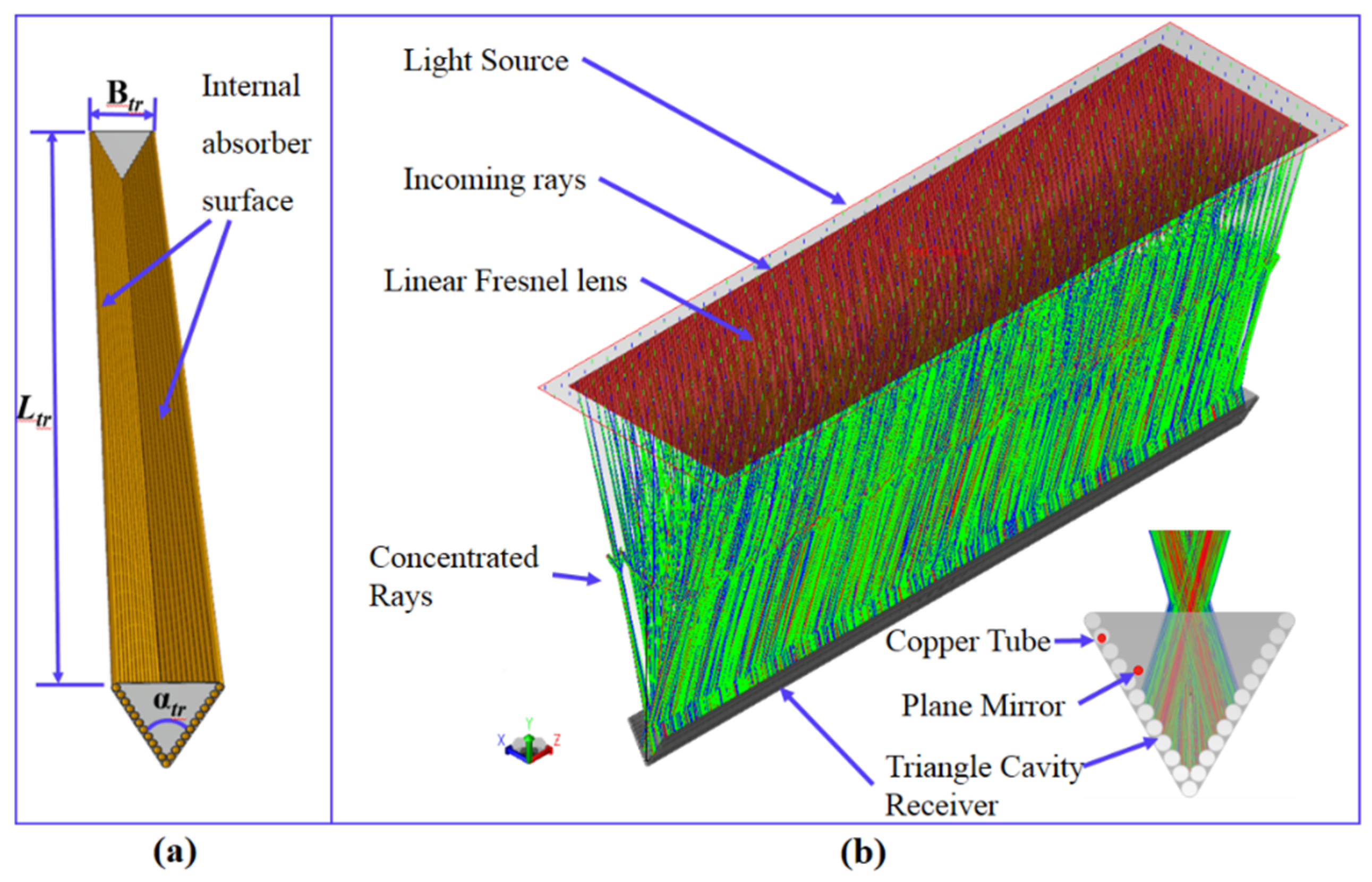
2.1. Physical Model

As illustrated in Figure 1, the FLFLSC was the integration of the sliding linear Fresnel lens with the fixed cavity receiver and the polar tracking system. It consists of a linear Fresnel lens, a fixed triangle cavity receiver, a sliding adjustment structure of lens element and a polar tracking system. The sunlight is focused on the internal surface of the fixed cavity receiver by the linear Fresnel lens with a sliding adjustment structure. The rotating polar axis in the tracking system is aligned parallel to the polar axis of the earth, and the linear focus of the linear Fresnel lens coincides with the polar axis to achieve a fixed focus line during sun tracking. The sun declination angle δ varies between −23.45° and +23.45° corresponding to the sun reaching its most southerly and northerly excursion relative to the celestial equator on the celestial sphere, respectively [18], and thus the incidence angle θ of direct solar radiation is less than 23.45°. As a polar tracking system was applied in the FLFLSC, that is, cos23.45° ≈ 0.917, the maximum cosine loss of the polar tracking method given by 1-cos23.45° will not exceed 8.3% [19], which means that the FLFLSC can effectively reduce the cosine loss of the system.

The key component, linear Fresnel lens is fabricated using polymethyl methacrylate (PMMA) through molding or extrusion with a clear texture. The digital photograph of FLFLSC shown is assembled from five small Fresnel lenses of length, width and thickness of 320, 400 and 2 mm, respectively. The groove pitch is 1 mm and the focal length is 650 mm. The grooves are placed facing downwards to reduce dust accumulation. The lenses are mounted in a slidable structure with sufficient rail length. Two triangular reflecting surfaces inside the triangular cavity are arranged as reflecting surfaces at both ends to reduce energy loss. Two surfaces inside the triangular cavity are arranged as receiving surfaces, which are two elongated rectangular surfaces. The cavity receiver absorbs the concentrated solar energy through the receiving surfaces that are made up of the outer surfaces of many copper tubes seamlessly joined together and transfers the heat to the working fluid through the copper tube. The working fluid flows in from the lower side of the cavity and flows out from the higher side, thereby taking away the heat. The geometric parameters include the lens element width B, lens element length L, focal length f₀ of FLFLSC, solar hour angle ω, sun declination angle δ and the horizontal angle of polar axis S₀. In this study, the S₀ is set to be 23°08′ based on the local latitude angle φ in Guangzhou, China.

The linear Fresnel lens is aligned in a north–south direction and rotates about the polaraxis to track the daily sun motion at the rotation angular velocity of the earth. In most operational conditions, direct solar radiation is not incidentally perpendicular to the surface of the linear Fresnel lens. Therefore, the incidence angle θ of direct solar radiation on the single-axis tracking array with a polar north–south-orientated, fixed linear-focus Fresnel lens solar concentrator, as shown in Figure 1, is obtained by the following formula [20,21]:

$$\cos \theta =\sin \delta \sin (\phi -S_0)+\cos \delta \cos (\phi -S_0)\cos \omega$$

(1)

Note that S₀ is equal to the φ, i.e., S₀ = φ. Moreover, the ω of direct solar radiation on the surface of the linear Fresnel lens is tracked all the time under ideal tracking conditions, i.e., ω = 0°. Applying the known conditions for Formula (1) we have:

$$\cos \theta =\cos \delta$$

(2)

Furthermore, the δ for any day of the year (N) can be presented approximately as [22,23],

$$\delta =23°27\prime \times \sin [\frac{360}{365}(284+N)]$$

(3)

For seasonal tracking, the element position of the linear Fresnel lens is manually adjusted with the aid of a screw rod mechanism. The lens element slips along the edge of the lens frame according to the δ until the offset linear focus does not exceed the end of the cavity receiver. For clarity, the principle sliding adjustment of Fresnel lens with change in incident angle of solar radiation is shown in Figure 2. When the sun rays shoot in with an oblique angle caused by the change of solar declination angle, the Fresnel lens is slid parallel until the concentrated sun rays reach one end of the triangle cavity receiver. Based on the linear Fresnel lens described in

Table 1. Parameters of FLFLSC using triangle cavity receiver for comparison.

Component	Parameter	Symbol	Value
Fixed linear linear-focus Fresnel lens solar concentrator	Lens element width	B	400 mm
	Lens element length	L	1500 mm
	Focal length	f0	650 mm
Triangle cavity receiver	Opening width	Btr	80 mm
	Opening length	Ltr	1500 mm
	Apex angle	αtr	60°
Solar source	Direct solar radiation value	Id	800 W/m2

, offset distance changes of the linear focal spot on the focal plane with the δ as the values shown in

Table 2. Offset distance changes of the linear focal spot with solar declination angle.

Item	Sun Declination Angle δ	Offset Distance (mm)
1	0°	0
2	8°	87
3	16°	183
4	23.45°	286

. The above models and methods can be transferred and applied to other countries and regions by adjusting design parameters and changing operating conditions.

2.2. Numerical Simulation Model

To estimate the solar flux distribution of triangle cavity receiver in the FLFLSC, commercial software TracePro^® using MCRT method was applied. It is an optomechanical software that provides professional service for design, optimization and evaluation for the optical and illumination systems [24]. Researchers use this tool extensively in solar optics applications [25]. The receiver employed in this study is a triangle cavity receiver constructed with a coated copper tube through which the heat transfer fluid flows, as shown in Figure 3a. The symbol B_tr, L_tr and α_tr denote the opening width, the opening length and the apex angle of the triangle cavity receiver, respectively. Various 3D models of the FLFLSC with different receiver positions, solar declination angles and solar hour angles are firstly modeled and assembled in UG 10.0 [26] and then imported into the TracePro^® to simulate the ray tracing process. In the proposed model, the surface reflectivity, transmittance and absorptivity characteristics of the triangle cavity receiver are set for each of the specific simulation conditions. However, the above surface characteristics of the linear Fresnel lens are set as constant.

It is necessary to establish some hypotheses before conducting the parametric study on the solar flux distribution of the solar concentrator since the optical performance research in this study is carried out in the perfect case. Engineering errors are not considered, including the slope, specular and contour errors of Fresnel lens; the alignment error of the triangular cavity receiver; and the tracking error of the system, etc. [27,28]. Once set the surface and geometry characteristics of the triangular cavity receiver will not change with the circumstances. To build a model close to reality, the half angular width of the sun is considered to be about 0.27° during simulation [29].

Figure 3b shows the ray-tracing analysis of a specific case. The ray-tracing process of a fixed linear-focus Fresnel lens coupled with a triangular cavity receiver can be seen clearly. The sunrays are refracted by the linear Fresnel lens and projected on the internal absorption surface of the triangle cavity receiver. Most of the incoming solar radiation energy can be absorbed after several reflections in the cavity. Finally, it is transferred to the working fluid through the copper tube after the absorption on the internal absorption surface. To minimize the optical loss at the end of the triangle cavity receiver, plane mirrors are arranged at both the ends of the triangle cavity receiver. The related parameters of FLFLSC using the triangle cavity receiver are listed in Table 1.

2.3. Optical Work Validation

To ensure the accuracy of the simulation, it is necessary to confirm the effectiveness of the simulation results based on the MCRT method by verifying the physical processes and methods used in this study. An indirect measurement system was designed for performance testing under real weather conditions to verify the simulation results.

In the experiment, the linear Fresnel lens is rotated to ensure that the solar radiation is incident vertically on the lens. The diffuse receiver is placed under the Fresnel lens parallel to the lens, or in other words, vertical to the direction of solar radiation. In order to verify the simulation results, an indirect measurement method was designed for performance testing under real weather conditions as shown in Figure 4. In the experiment, the linear Fresnel lens is rotated to ensure that the solar radiation is incident vertically with Fresnel lens grooves facing downwards. The target is a white Lambert board with dimensions of 300 mm by 320 mm square produced by Labsphere Company of U.S. The diffuse receiver is placed under the Fresnel lens parallel to the lens, or in other words, vertical to the direction of sunlight. The CCD camera is a detector with 2048 by 4096 pixels enabling high resolution images of focal line. There are two types of indirect measuring methods including on-axis and off-axis. The former means that the symmetry axis of the CCD camera overlaps with the vertical lines of the receiver plane. The other one is to make the vertical line of the receiving surface at a small angle to the central axis of the CCD camera. In order to avoid forming a CCD camera shadow on the diffuse receiver, the off-axis measurement is done. The deflection angle β is limited to 3° by which way the error caused by Lambert attributes can be ignored [30].

We calibrated the angle and position of the CCD camera before taking the shot, and then captured the focused linear facula. The flux distribution of the focus facula can be obtained by the data acquisition system, which can correct the distortion of the image, change the coordinate unit and convert the grayscale of the image into the flux intensity [29]. The flux distribution of the focus facula measured under actual conditions is shown in Figure 5a. Referring to Figure 5b, it will be understood that the simulated flux distribution has a similar result, the width of the main facula and the facula, respectively, are about 26 mm and 84 mm. When the direct radiation value is 796 W/m², the maximum flux density on the planar receiver according to the experimental and simulated results are 18,137 and 19,052 W/m², respectively.

In order to compare the experimental and simulation results, the flux distribution at five horizontal lines of the focus facula was selected for analysis, and the curves of the average flux density on five horizontal lines are shown in Figure 6 [31]. In the area within the main facula, the experimental and simulation results are basically consistent with each other. The areas enclosed by the experimental and simulated curves, respectively, are S₀ and S₀’. The relative error between them is 3.24%. In the area within the width of the facula, the experimental results of side facula are larger than that of simulation, but the error is not significant. The areas enclosed by the experimental and simulated curves, respectively, are S₁ and S₁’, and the relative error between them is 15.35%. It may be due to a manufacturing error, surface scattering and the teeth rounded edges of the linear Fresnel lens and the disparity between the response of the solar spectrum and the CCD camera, etc. The present numerical procedure matched closely with the experimental data.

TracePro^® is incorporated into the simulation of the flux distribution on the triangular cavity receiver. As the resulting precision is decided by the total number of trace rays emitted by the light source, it is necessary to find out the most appropriate number of rays. Initial ray numbers of 7300, 32,100, 72,100, 128,900 and 203,900 were set during the simulation on the optical efficiency of the FLFLSC using a triangular cavity receiver with θ = 0°. For each of rays, the total energy is the same. As the total energy of sun rays for five different ray numbers is the same, the energy allocated to each ray is different. The less the number of sun rays, the more energy each ray carries, and the more likely it is to cause a high concentration of energy. Furthermore, the fewer the number of sun rays, the greater the possibility of error. Conversely, if the number of sun rays is larger, the less likely it is to cause errors, and the more the simulation result closes to the real situation. Figure 7 shows the flux distribution along the width of the receiver internal surface. Compared to other numbers of rays, the value of heat flux for 7300 rays is more than twice due to the more carried energy of each ray causing a high concentration of energy.

Figure 8 shows the relative deviation of heat flux distribution values between the results of the 203,900 rays and the other four number of rays. It can be distinguished easily that most of the ray numbers showed little deviations with the number of 203,900 in the flux distribution except for 7300 rays. The maximal relative deviation of heat flux detected in Figure 8 is about 0.126, when 128,900 rays are set. Moreover, the calculated optical efficiency of the FLFLSC using the triangular cavity receiver in the case of θ = 0° in the 128,900 rays and the 203,900 rays is 77.93%. Therefore, 128,900 rays are used to simulate the optical performance of FLFLSC using a triangular cavity receiver.

2.4. Uniformity Factor (UF)

For comparison, the flux uniformity of the receiver internal surface is defined by a uniformity factor (UF) as indicated below [32]:

$$UF=1-\frac{MaximumFlux-AverageFlux}{MaximumFlux}$$

(4)

The maximum flux is defined as the peak value collected during the experiment or simulation, while the average flux is calculated by dividing the incident and absorbed energy by the area of receiver internal surface.

2.5. Simulation Method

The simulation process is completed by the software TracePro^®. During the process, the parameters such as solar declination angle δ, solar hour angle ω, the vertical distance between the opening plane of the cavity and the Fresnel lens f, the internal surface absorptivity α_ab and the end plane reflectivity ρ_r are changed individually. The value of δ varies from −23.45° to +23.45° throughout the year. Due to symmetry factors, only δ values in the range of 0 to +23.45° are studied. The observation points are set at an interval of 8°. Thus, the δ is set as 0°, +8°, +16° and +23.45°. The performance of the FLFLSC is examined for planning to explore the performance of the small FLFLSC during the four hours before and after noon, which means a total of eight hours of sunlight during the day. Similarly, due to symmetry, the solar hour angle range of 0°–60° is investigated. The observation points are set at an interval of 15°. Thus, the solar hour angle is set as 0°, 15°, 30°, 45° and 60°. Since the focal length of the Fresnel lens is 650 mm, the vertical distance between the opening plane of the cavity and the Fresnel lens f is set as 600 mm, 625 mm, 650 mm, 675 mm and 700 mm. In order to simulate the real situation as much as possible, the internal surface absorptivity α_ab is set as 0.75, 0.85 and 1.00. The end plane reflectivity ρ_r is set as 0.75, 0.85 and 1.00.

For each case, the controlling variable method is adopted. For example, when the date varies to a specific day, the value of δ is +8°and the solar hour angle is gradually varied, with other parameters kept constant. The software is run, and the light distribution and the cavity receiver energy distribution are obtained through the built-in program. The energy distribution on the area of two elongated rectangular surfaces inside the triangle cavity is counted. The performance of the small FLFLSC on a specific day can be obtained in this way. The influence of every parameter can be acquired by changing the parameter value and rerunning the software. Note that when the δ changes, the Fresnel lens is slipped parallel for an appropriate distance to make sure that the focal line slide does not exceed the cavity receiver.

3. Results and Discussion

The primary purpose of this study is to investigate the solar flux uniformity of the triangle cavity receiver in FLFLSC under various sunlight incidence angles and to find the optimal parameters of the receiver aiming to improve the UF of the triangle cavity receiver. The parameters are receiver position (f), receiver internal surface absorptivity (α_ab) and end reflection plane reflectivity (ρ_r). The ω and the δ have been taken into consideration in the following cases for showing the effect of receiver parameters on the UF of the triangle cavity receiver objectively.

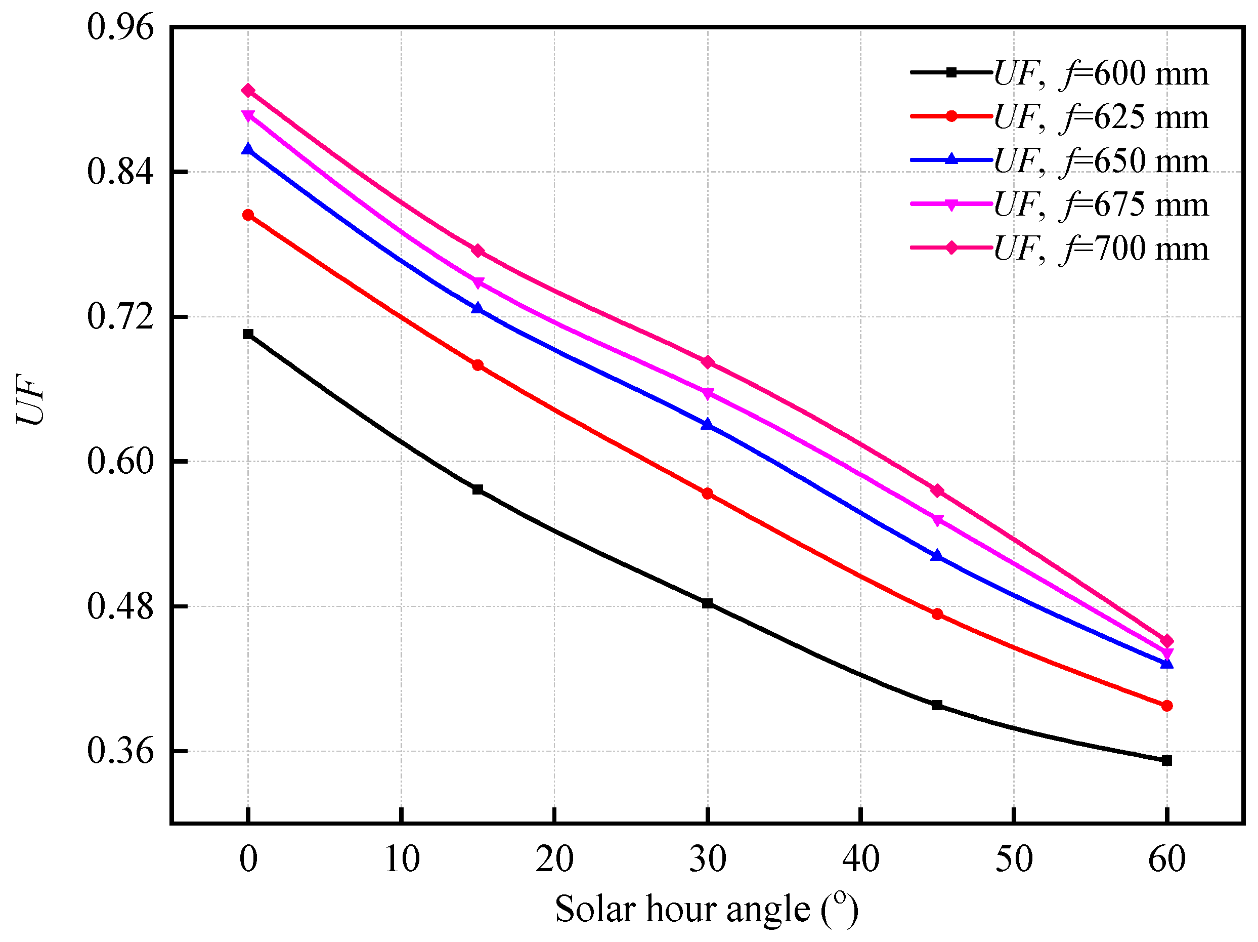
3.1. Effect of Receiver Position f

The effect of shifting the receiver position is intensely investigated. Figure 9, Figure 10, Figure 11 and Figure 12 show the results of five studied positions for the triangle cavity receiver when the α_ab and ρ_r are both 0.85. As shown in Figure 9, when the δ is 0°, the effect of the receiver position is clearly seen. The UF has a sensitivity to various values of f as the UF between them is significantly different for ω of 0–60°. Moreover, the larger the value of f, the larger the UF is. As can be seen from the size of the interval between the curves that after f is greater than 650 mm, the UF rises faster. It may be explained that when f is in the range of 600–650 mm, the linear focus can be basically enclosed in the cavity, but when f exceeds 650 mm, the width of focused linear facula raises, resulting in a higher UF value.

It is worth noting that the interval between the f = 600 mm curve and other f mainly increase first for the ω of 0–15° and then decreases as ω further increases in the range of 15–60°, even if there is overlap between the curves f = 600 and 625 mm for ω of 35–60°. It is because that the focused light is initially distributed on the two absorption surfaces of the cavity, and then gradually concentrated on only one of the surfaces. The apex angle of triangle cavity receiver plays an essential role during the transferring since the sun rays concentrate here causing the low ebb on the curves of f = 600 and 625 mm. The low ebb can be observed only in the above two curves, which suggests that the concentrating effect should be considered while using a small f.

As mentioned previously, UF is positively correlated with f for the ω of 0–60°. The reason is that the larger f is, the farther the focal line is from the bottom of the triangular cavity. On the contrary, the smaller the f, the closer the focal line is to the apex angle of triangle cavity, which causes the received solar energy to accumulate since the bottom area of the triangular cavity is small. In other words, increasing f can make the energy flow density uniform. The UF curves with f = 600 and 625 mm decrease first for ω about 0–20°, then increase for ω about 20–30°, then finally decrease with the increasing of ω between 30° and 60°. It can be inferred that the amount of sun rays received by the two sides of the receiver’s internal surface is basically unchanged for ω about 20–30°, but the total area receiving the concentrated sun rays becomes larger, which leads to the decrease of the maximum flux. The average UF for the triangle cavity receiver with f = 600, 625, 650, 675 and 700 mm, respectively, are 0.3054, 0.3166, 0.3539, 0.4096 and 0.4813 for the ω of 0–60°. The triangle cavity receiver with f = 700 mm has the highest average UF in one day as the δ = 0°, compared to other receiver positions.

Similar behavior can also be observed in Figure 10, when the value of δ is 8°. Note that UF increases with f and the interval of the UF between two neighboring curves increases with f in the range of 600–700 mm for the ω of 0–50°. In addition, except for the UF curve of f = 600 mm, the other curves basically decrease as ω raises in the range of 0–60°. Additionally, the rate of decline is gradually slowed down. The UF curve with f = 700 mm drops approximately linearly. The overall change in the trend of each curve with a δ value of 8° is similar to the curve with a δ value of 0°, but there are slight differences. It is observed that the value of δ also influences UF in Figure 9 and Figure 10. Additionally, the average UF for the triangle cavity receiver with f = 600, 625, 650, 675 and 700 mm, respectively, are 0.3081, 0.3316, 0.3860, 0.4460 and 0.5173 under the ω between 0° and 60° when the value of δ is 8°. They are higher than the corresponding average UF values when the δ is 0°. This is because when the sun declination angle increases, the focal line has an upward displacement making the focal line farther from apex at the bottom, but this may result in a decrease in optical efficiency.

In the same way, Figure 11 shows the effect of changing the triangle cavity receiver position under different ω when the δ is 16°. As can be observed, the UF is sensitive to the different preset f as the difference between UF curves are significant for ω about 0–60°. The interval between the curves is different before and after a ω value of 30°. The δ is inferred to play a crucial role on the UF. The intervals of the UF between f = 600 mm curves and other f values increase firstly for the ω of 0–15° and then decrease in the range of 15–60°. The interesting thing is that can be found that the larger the f is, the larger the decrease in UF for ω in 0–60° range. It can be seen that the curves are dispersed at the beginning and converge gradually. When ω is 60°, the curves are relatively close to each other, especially the curves with f values of 650, 675 and 700 mm. This is because the focal line moves up further with the increase of δ. This upward movement combined with the reflection of the cavity reduces the influence of f. The average UF values for the triangle cavity receiver with f = 600, 625, 650, 675 and 700 mm, respectively, are 0.3534, 0.4143, 0.4818, 0.5341 and 0.5865 for the ω of 0–60° with a δ value of 16°.

Figure 12 illustrates the effect of changing the triangle cavity receiver position under different ω when the δ is 23.45°. It can be found that the UF is sensitive to the different preset f for ω in the range of 0–60°. Additionally, the intervals in the UF between two neighboring curves decrease with the increasing of the f in the range of 600–700 mm. It is because the linear focus is outside the triangle cavity receiver for the f of 600–700 mm, the area receiving the concentrated sun rays on internal absorption surface does not increase significantly with the increase of the f in the range of 600–700 mm. It is worth noting that the differences of the UF between f = 600 mm and other f mainly increase firstly for the ω of 0–30° and then decrease in the range of 30–60°, but the size of the interval hardly fluctuates. In addition, the UF curves basically decrease linearly with the increase in ω for the range of 0–60°. Moreover, the average UF for the triangle cavity receiver with f = 600, 625, 650, 675 and 700 mm, respectively, are 0.5030, 0.5858, 0.6337, 0.6576 and 0.6784 under the ω between 0° and 60° with a δ value of 23.45°. From the changes in the UF at different δ in Figure 9, Figure 10, Figure 11 and Figure 12, it can be found that the solar flux uniformity of triangle cavity receiver improves as the δ increases, and deteriorates as the ω increases.

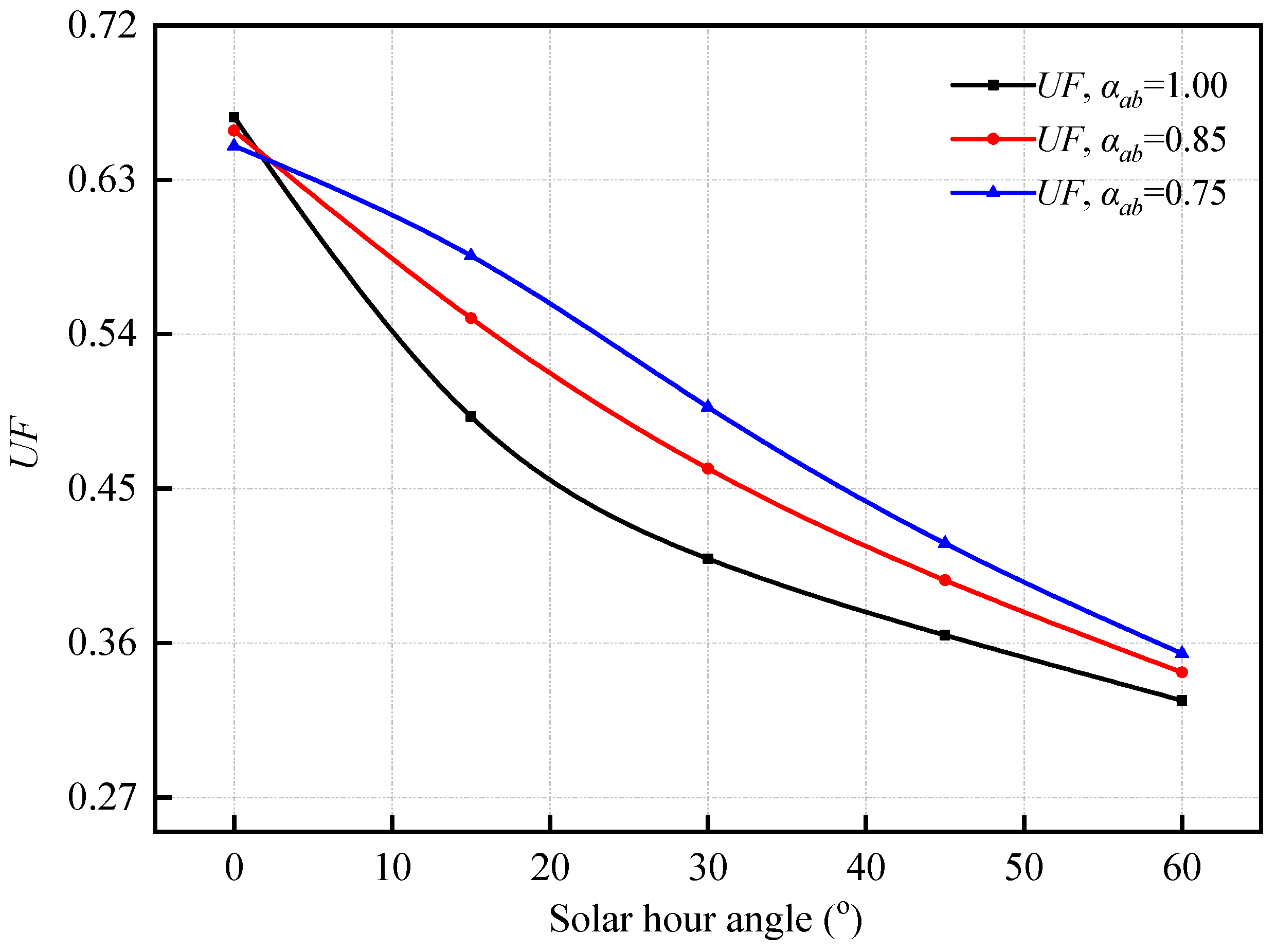
3.2. Effect of Receiver Internal Surface Absorptivity α_ab

Figure 13 and Figure 14 show the results of the receiver internal surface absorptivity influences for the UF of triangle cavity receiver based on ρ_r = 0.85 and f = 650 mm. Figure 13 illustrates the effect of α_ab on the UF of triangle cavity receiver under various ω, when the δ is 0°. The simulation results were obtained with α_ab values of 1.00, 0.85 and 0.75. It can be detected that the different preset α_ab of the triangle cavity receiver has an influence on the UF as the values of UF between them are significantly different. Note that the interval of the UF between α_ab values of 1.00 and 0.85 is larger than that between α_ab values of 0.85 and 0.75 for the ω in the range of 0–60°. Moreover, the differences of the UF between α_ab value of 1.00 and other α_ab mainly increase first for the ω of 0–25° and then decrease in the range of 25–60°. It is because that the concentrated sun rays can be basically received after many times of absorption and reflection between the two sides of the receiver internal surface in the triangle cavity receiver when the ω is between 0° and 25°. Since the triangular cavity has two receiving surfaces, the light concentrates on one of the receiving surfaces when the value of ω changes. By lowering the value of α_ab, more energy can be reflected to the other receiving surface, improving the uniformity of energy receiving and thus increasing the UF. The improvement was more pronounced when the light was more concentrated on one surface. In addition, the concentrated sun rays are mainly concentrated on one side of the receiver internal surface for the ω in the range of 25–60°, sun rays that have not been absorbed for one time begin to escape from the triangle cavity receiver and the number of escaped sun rays increases with the increasing of ω. Thus, the influence of α_ab on the UF decreases gradually with the increase of ω. It may be revealed that the ω also influences UF.

It also can be found that the UF decreases with the increase of α_ab for the ω in the range of 0–60°. This was because the concentrated sun rays are mainly received, absorbed and reflected between the two sides of the receiver internal surface in the triangle cavity receiver, thus, the lower the α_ab, the more the number of concentrated sun rays reflected and absorbed, and the greater the distribution of the concentrated sun rays absorbed on the receiver internal surface. The UF of different value of α_ab firstly falls sharply and decreases slowly with the increase of ω before and after a ω value of 30°. It may be inferred that the influence of ω on the UF before the ω reaches 30° is stronger than when it exceeds 30°. The average UF for the triangle cavity receiver of α_ab = 1.00, 0.85 and 0.75, respectively, are 0.3302, 0.3539 and 0.3719 under the ω between 0° and 60°.

Similar behavior also can be noticed in Figure 14, when the δ is 8°. The introduced triangle cavity receivers of different α_ab have an influence on the UF as the differences of UF between them are significant. The differences in the UF between α_ab = 1.00 and 0.85 are larger than that between α_ab = 0.85 and 0.75 for the ω of 0–60°. Moreover, the differences of the UF between α_ab = 1.00 and other α_ab mainly increase first for the ω of 0–25° and then decrease with the increasing of ω in the range of 25–60°. It also can be seen that the UF decreases as the α_ab increases for the ω of 0–60°. Additionally, the UF of different α_ab first falls sharply and decreases slowly with the increase of ω before and after a ω value of 30°. The average UF for the triangle cavity receiver of α_ab = 1.00, 0.85 and 0.75, respectively, are 0.3552, 0.3818 and 0.4005 under the ω between 0° and 60°. In short, the curves of the UF with different α_ab when the δ is 8° are basically the same as that when the δ is 0°. It means that the increase in the δ cannot significantly improve the UF based on ρ_r = 0.85 and f = 650 mm when the δ is between 0° and 8°. In other words, the δ has little influence on UF when δ is 0–8°.

Likewise, Figure 15 shows the effect of changing receiver internal surface absorptivity of the triangle cavity receiver under different ω when the δ is 16°. The different preset α_ab of triangle cavity receivers has an influence on the UF as the differences of UF between them are significant. Note that the differences of the UF between α_ab 1.00 and other α_ab mainly decrease first for the ω of 0–3°, then increase for the ω of 3–25°, and finally decrease with the increasing of ω in the range of 25–60°. It also can be seen that the UF increases and decreases, respectively, as the α_ab increases before and after the ω value of 3°. It may be because that when the δ is 16°, the concentrated sun rays after being refracted by the linear Fresnel lens obliquely enter the triangle cavity receiver, and the inclination angles of the concentrated sun rays are relatively large, causing the sun rays to be concentrated toward the end of receiver internal surface after being reflected. When the ω is fixed, the lower the α_ab, the more obvious this situation is.

However, as the ω increases, the concentrated sun rays gradually gather from two sides to one side of receiver internal surface, thus the above situation is weakened. It may be inferred that the ω has a more significant influence on the UF, compared to the δ. Moreover, the UF of α_ab = 1.00 and 0.85 firstly falls sharply and decreases slowly with the increasing of ω before and after a ω value of 30°. The average UF for the triangle cavity receiver of α_ab = 1.00, 0.85 and 0.75, respectively, are 0.4517, 0.4818 and 0.5009 under the ω between 0° and 60°.

Figure 16 shows the effect of changing receiver internal surface absorptivity of the triangle cavity receiver at different ω when the δ is 23.45°. It can be found that the UF has a sensitivity to the introduced triangle cavity receiver of various α_ab as the UF between them are significant for ω about 0–60°. However, the differences of the UF between α_ab = 1.00 and other α_ab mainly decrease first for the ω of 0–10°, then increase for the ω of 10–30°, and finally decrease as the ω increases in the range of 30–60°. It also can be seen that the UF increase and decrease, respectively, with the increasing of α_ab before and after the ω value of 10°. It means that more sun rays have been concentrated toward the end of receiver internal surface after being reflected when the δ is 23.45°.

Besides, the UF curves decrease with the increasing of ω in the range of 0–60°, but the downward trend of the UF curves with α_ab = 1.00, 0.85 and 0.75, respectively, decreases when unchanged and increases with the increase of ω in the range of 0–60°. It means that the δ also influences UF. Moreover, the average UF for the triangle cavity receiver of α_ab = 1.00, 0.85 and 0.75, respectively, are 0.6024, 0.6277 and 0.6397 under the ω between 0° and 60°. From the changes in the UF at different δ in Figure 13, Figure 14, Figure 15 and Figure 16, it can be concluded that the solar flux uniformity is improved by the lower α_ab as the concentrated sun rays are reflected mainly on both sides of the receiver internal surface.

3.3. Effect of End Reflection Plane Reflectivity ρ_r

Figure 17 and Figure 18 present the effect of end reflection plane reflectivity ρ_r on the UF of the triangle cavity receiver under various values of ω at four different solar declination angle δ = 0°, 8°, 16° and 23.45°, respectively. In Figure 17, the effect of changing ρ_r under different ω can be observed as the δ is set to 0° and 8°. The different preset ρ_r of triangle cavity receiver does not influence the UF because the UF curves of them basically coincide. Moreover, the UF of different ρ_r first falls sharply and decreases slowly with the increasing of ω before and after a ω value of 30°, respectively. However, the differences of the UF between the triangle cavity receivers with different ρ_r are significant for ω about 0–30° and 0–40° when the δ, respectively, are 16° and 23.45°, as shown in Figure 18. It may be inferred that the concentrated sun rays are mainly reflected and absorbed between the two sides of receiver internal surface when the δ is between 0° and 8°.

However, the concentrated sun rays gradually concentrate toward the end of receiver internal surface after being reflected as the δ increases. Some sun rays are absorbed by the end of receiver internal surface after being reflected by the end reflection plane. When the δ and ω are fixed, the lower the ρ_r, the more pronounced this situation is. There is a difference in the effect of ρ_r on UF at a δ value of 16° and 23.45° at a ω value of 0°. It means that as the value of δ increases, the number of sun rays reflected from the end of receiver internal surface to the end reflection plane increases, resulting in an increase in the number of sun rays reflecting back to the end of receiver internal surface through the end reflection plane, increasing the local energy flow density, and finally resulting in a decrease in UF. Nevertheless, as the ω increases, the concentrated sun rays gradually gather from both sides to one side of receiver internal surface, thus the above situation is weakened. It may be inferred that the ω has a more significant influence on the UF, compared to the δ. In addition, the UF of different α_ab basically declines linearly with the increasing of ω between 0° and 60°. Nevertheless, for comparison’s sake, the average UF under different ρ_r were calculated when the δ were 0°, 8°, 16° and 23.45°. The average UF under different ρ_r for the triangle cavity receiver of δ = 0°, 8°, 16° and 23.45°, respectively, are 0.4074, 0.4403, 0.5550 and 0.7349 under the ω between 0° and 30°. Moreover, the average UF under different ρ_r for the triangle cavity receiver of δ = 0°, 8°, 16° and 23.45°, respectively, are 0.3539, 0.3810, 0.4809 and 0.7349 under the ω between 0° and 60°.

3.4. Analysis of Variance

Though the UF of FLFLSC using triangle cavity receiver is the-larger-the-better, it is also affected by various factors. To evaluate the level of each impact factor on the UF of triangle cavity receiver and provide a more intuitive judgment basis for the significance of various factors, the analysis of variance (ANOVA) was used.

Table 3. Controlling factors of the analysis of variance and their levels.

Level	Experiment Factor
	f (A)	αab (B)	ρr (C)	δ (D)	ω (E)
1	600 mm	1.00	1.00	0°	0°
2	625 mm	0.85	0.85	8°	15°
3	650 mm	0.75	0.75	16°	30°
4	675 mm	/	/	23.45°	45°
5	700 mm	/	/	/	60°

shows the design of various controlling factors and corresponding levels based on the full-factorial orthogonal array. Five factors that include one 4-level factor (δ), two 5-level factors (f and ω) and two 3-level factors (α_ab and ρ_r) can be seen in it. Therefore, the experiment was conducted 4 × 5² × 3² times (i.e., 900 times).

Table 4. Analysis of variance for uniformity factor.

Source	SS #	df	MS	F-Value	p-Value
Model	19.401 a	15	1.293	127.954	<0.0001
A	2.788	4	0.697	68.957	<0.0001 *
B	0.337	2	0.169	16.678	<0.0001 *
C	0.006	2	0.003	0.278	0.757
D	4.744	3	1.581	156.445	<0.0001 *
E	11.552	4	2.888	285.702	<0.0001 *
Error	8.926	883	0.010	/	/
Total	210.753	900	/	/	/

^# SS—sum of squares; df—degree of freedom; MS—mean square. ^a R² = 0.685, R² (adjusted) = 0.680. * means significant (p-Value < 0.01).

lists the ANOVA of the quadratic model on UF. Adequate precision measures the signal to noise ratio, and R² indicates the coefficient of multiple determination [33,34]. R² = 0.685 indicates that the quadratic model can explain 68.5% of the variance in the response. The large F-value of the model (127.954) implies the great significance of the regression model. The associated p-value is less than 0.05 and greater than 0.1, respectively, indicating that the model item is statistically significant and the effects of the model terms are not significant. Therefore, in addition to the factor C (ρ_r), other factors have a very significant impact on UF.

According to the SS in Table 4, factor E (ω) has the most significant influence on the UF, followed by factor D (δ), factor A (f) and factor B (α_ab). Though δ and ω affect the most in the UF, by the time the solar concentrator is completed, the δ and ω have been fixed, and the high α_ab of the coating material will lead to high costs of solar concentrator production. Thus, combined with the annual and temporal variability of solar radiation in the location of the solar energy system, placing the triangle cavity receiver in an appropriate position is a means that considers both economy and effectiveness to improve the UF. Consequently, the FLFLSC using triangle cavity receiver with a α_ab value of 0.85 and a ρ_r value of 0.75 is selected, and the average UF for the ω of 0–60° at different f and different δ is calculated, as shown in Figure 19.

It can be found that when the f is fixed, the average UF increases with the increasing of the δ, but the average UF increases with the increasing of the f when the δ is fixed, except for the δ value of 23.45°. Note that when the δ is 23.45°, the average UF firstly increases then decreases and finally increases with the increasing of the f. It is mainly because when the f is between 600 and 650 mm, some areas at the concentrated side of triangle cavity receiver have no incident concentrated sun rays, but it decreases as f increases, resulting in an increase in average UF. When the f is between 650 and 675 mm, the area of no incident concentrated sun rays at the non-concentrated side of triangle cavity receiver increases with the increasing of the f, resulting in a decrease in average UF. When the f is between 600 and 650 mm, although the area of no incident concentrated sun rays at the non-concentrated side of triangle cavity receiver is further increased. However, the density of incident concentrated sun rays decreases with the increase of the f, resulting in a decrease in the maximum flux density formed at the concentrated side of triangle cavity receiver, which in turn leads to an increase in average UF.

4. Conclusions

In the present research, based on the application of linear Fresnel lens in the linear concentrating solar collector, a fixed linear-focus Fresnel lens solar concentrator (FLFLSC) is proposed. In order to investigate and optimize the solar flux uniformity of FLFLSC using triangle cavity receiver under various sun incidence angles, the effects of receiver parameters were studied. The main results are summarized as follows:

(1) The increase in the f will gradually weaken the solar flux uniformity improvement with the increasing of δ. When the δ is 0°, the average UF for the triangle cavity receiver with f = 600, 625, 650, 675 and 700 mm, respectively, are 0.3054, 0.3166, 0.3539, 0.4096 and 0.4813 under the ω between 0° and 60°. When the δ is 23.45°, the average UF for the triangle cavity receiver with f = 600, 625, 650, 675 and 700 mm, respectively, are 0.5030, 0.5858, 0.6337, 0.6576 and 0.6784 under the ω between 0° and 60°.

(2) The UF of triangle cavity receiver increases with the decreases of α_ab when other receiver parameters are fixed, but the influence of α_ab on it gradually weakens with the increase of δ and even produces the opposite effect. When the δ is 0°, the average UF for the triangle cavity receiver of α_ab = 1.00, 0.85 and 0.75, respectively, are 0.3302, 0.3539 and 0.3719 under the ω between 0° and 60°. When the δ is 23.45°, the average UF for the triangle cavity receiver of α_ab = 1.00, 0.85 and 0.75, respectively, are 0.6024, 0.6277 and 0.6397 under the ω between 0° and 60°.

(3) The ρ_r cannot affect the solar flux uniformity of the triangle cavity receiver, unless the δ are relatively large and the ω are relatively small, causing some concentrated sun rays to be reflected by the plane mirror. The average UF under different ρ_r for the triangle cavity receiver of δ = 0°, 8°, 16° and 23.45°, respectively, are 0.3539, 0.3810, 0.4809 and 0.7349 under the ω between 0° and 60°.

(4) From the significance test of critical factors on the UF of FLFLSC using triangle cavity receiver, the ω has the most significant influence on the UF, followed by δ, f and α_ab. Choosing the appropriate position of the triangle cavity receiver is the most cost-effective means to improve the UF due to the determined δ and ω when the design of the solar concentrator is completed and the coating materials having excessively high α_ab lead to an increase in the costs of solar concentrator production.

References

1. Bhusal, Y.; Hassanzadeh, A.; Jiang, L.; Winston, R. Technical and economic analysis of a novel low-cost concentrated medium-temperature solar collector. Renew. Energy 2020, 146, 968–985. [Google Scholar] [CrossRef]
2. Sarwar, J.; Shad, M.R.; Hasnain, A.; Ali, F.; Kakosimos, K.E.; Ghosh, A. performance analysis and comparison of a concentrated photovoltaic system with different phase change materials. Energies 2021, 14, 2911. [Google Scholar] [CrossRef]
3. Pasupathi, M.K.; Alagar, K.; P, M.J.S.; M.M, M.; Aritra, G. Characterization of hybrid-nano/paraffin organic phase change material for thermal energy storage applications in solar thermal systems. Energies 2020, 13, 5079. [Google Scholar] [CrossRef]
4. Diao, R.; Sun, L.; Yang, F.; Lin, B. Performance of building energy supply systems using renewable energy. Int. J. Energy Res. 2020, 44, 9960–9973. [Google Scholar] [CrossRef]
5. Liu, B.; Zhang, X.; Ji, J. Review on solar collector systems integrated with phase-change material thermal storage technology and their residential applications. Int. J. Energy Res. 2021, 45, 8347–8369. [Google Scholar] [CrossRef]
6. Mukhtar, M.; Ameyaw, B.; Yimen, N.; Quixin, Z.; Bamisile, O.; Adun, H.; Dagbasi, M. Building retrofit and energy conservation/efficiency review: A techno-environ-economic assessment of heat pump system retrofit in housing stock. Sustainability 2021, 13, 983. [Google Scholar] [CrossRef]
7. Gulaliyev, M.G.; Mustafayev, E.R.; Mehdiyeva, G.Y. Assessment of solar energy potential and its ecological-economic efficiency: Azerbaijan case. Sustainability 2020, 12, 1116. [Google Scholar] [CrossRef] [Green Version]
8. Fuqiang, W.; Ziming, C.; Jianyu, T.; Yuan, Y.; Yong, S.; Linhua, L. Progress in concentrated solar power technology with parabolic trough collector system: A comprehensive review. Renew. Sustain. Energy Rev. 2017, 79, 1314–1328. [Google Scholar] [CrossRef]
9. Sing, C.K.L.; Lim, J.S.; Walmsley, T.G.; Liew, P.Y.; Goto, M.; Salim, S.A.Z.B.S. Time-dependent integration of solar thermal technology in industrial processes. Sustainability 2020, 12, 2322. [Google Scholar] [CrossRef] [Green Version]
10. Zhai, H.; Dai, Y.; Wu, J.; Wang, R.; Zhang, L. Experimental investigation and analysis on a concentrating solar collector using linear Fresnel lens. Energy Convers. Manag. 2010, 51, 48–55. [Google Scholar] [CrossRef]
11. Qiu, Y.; Li, M.; Wang, K.; Liu, Z.; Xue, X. Aiming strategy optimization for uniform flux distribution in the receiver of a linear Fresnel solar reflector using a multi-objective genetic algorithm. Appl. Energy 2017, 205, 1394–1407. [Google Scholar] [CrossRef] [Green Version]
12. Prasad, G.C.; Reddy, K.S.; Sundararajan, T. Optimization of solar linear Fresnel reflector system with secondary concentrator for uniform flux distribution over absorber tube. Sol. Energy 2017, 150, 1–12. [Google Scholar] [CrossRef]
13. Wang, G.; Chen, Z.; Hu, P.; Cheng, X. Design and optical analysis of the band-focus Fresnel lens solar concentrator. Appl. Therm. Eng. 2016, 102, 695–700. [Google Scholar] [CrossRef]
14. Pham, T.T.; Vu, N.H.; Shin, S. Novel design of primary optical elements based on a linear Fresnel lens for concentrator photovoltaic technology. Energies 2019, 12, 1209. [Google Scholar] [CrossRef] [Green Version]
15. Lin, M.; Sumathy, K.; Dai, Y.; Zhao, X. Performance investigation on a linear Fresnel lens solar collector using cavity receiver. Sol. Energy 2014, 107, 50–62. [Google Scholar] [CrossRef]
16. Zhao, D.; Xu, E.; Wang, Z.; Yu, Q.; Xu, L.; Zhu, L. Influences of installation and tracking errors on the optical performance of a solar parabolic trough collector. Renew. Energy 2016, 94, 197–212. [Google Scholar] [CrossRef]
17. FuQiang, W.; Jianyu, T.; Lanxin, M.; Chengchao, W. Effects of glass cover on heat flux distribution for tube receiver with parabolic trough collector system. Energy Convers. Manag. 2015, 90, 47–52. [Google Scholar] [CrossRef]
18. Jamil, B.; Bellos, E. Development of empirical models for estimation of global solar radiation exergy in India. J. Clean. Prod. 2019, 207, 1–16. [Google Scholar] [CrossRef]
19. Yao, Y.; Hu, Y.; Gao, S.; Yang, G.; Du, J. A multipurpose dual-axis solar tracker with two tracking strategies. Renew. Energy 2014, 72, 88–98. [Google Scholar] [CrossRef]
20. Herrera-Romero, J.V.; Colorado-Garrido, D.; Soberanis, M.E.; Flota-Bañuelos, M. Estimation of the optimum tilt angle of solar collectors in Coatzacoalcos, Veracruz. Renew. Energy 2020, 153, 615–623. [Google Scholar] [CrossRef]
21. Al-Taani, H.; Arabasi, S. Solar irradiance measurements using smart devices: A cost-effective technique for estimation of solar irradiance for sustainable energy systems. Sustainability 2018, 10, 508. [Google Scholar] [CrossRef] [Green Version]
22. Eldin, S.S.; Abd-Elhady, M.S.; Kandil, H.A. Feasibility of solar tracking systems for PV panels in hot and cold regions. Renew. Energy 2016, 85, 228–233. [Google Scholar] [CrossRef]
23. Almutairi, K.; Mostafaeipour, A.; Jahanshahi, E.; Jooyandeh, E.; Himri, Y.; Jahangiri, M.; Issakhov, A.; Chowdhury, S.; Dehshiri, S.H.; Dehshiri, S.H.; et al. Ranking locations for hydrogen production using hybrid wind-solar: A Case Study. Sustainability 2021, 13, 4524. [Google Scholar] [CrossRef]
24. Pavlovic, S.; Bellos, E.; Loni, R. Exergetic investigation of a solar dish collector with smooth and corrugated spiral absorber operating with various nanofluids. J. Clean. Prod. 2018, 174, 1147–1160. [Google Scholar] [CrossRef]
25. Abed, N.; Afgan, I. An extensive review of various technologies for enhancing the thermal and optical performances of parabolic trough collectors. Int. J. Energy Res. 2020, 44, 5117–5164. [Google Scholar] [CrossRef] [Green Version]
26. Li, S.; Xu, G.; Luo, X.; Quan, Y.; Ge, Y. Optical performance of a solar dish concentrator/receiver system: Influence of geometrical and surface properties of cavity receiver. Energy 2016, 113, 95–107. [Google Scholar] [CrossRef]
27. Wang, H.; Huang, J.; Song, M.; Yan, J. Effects of receiver parameters on the optical performance of a fixed-focus Fresnel lens solar concentrator/cavity receiver system in solar cooker. Appl. Energy 2019, 237, 70–82. [Google Scholar] [CrossRef]
28. Li, C.; Lyu, Y.; Li, C.; Qiu, Z. Energy performance of water flow window as solar collector and cooling terminal under adaptive control. Sustain. Cities Soc. 2020, 59, 102152. [Google Scholar] [CrossRef]
29. Wang, H.; Huang, J.; Song, M.; Hu, Y.; Wang, Y.; Lu, Z. Simulation and experimental study on the optical performance of a fixed-focus Fresnel lens solar concentrator using polar-axis tracking. Energies 2018, 11, 887. [Google Scholar] [CrossRef] [Green Version]
30. Wu, G.; Zheng, H.; Ma, X.; Kutlu, C.; Su, Y. Experimental investigation of a multi-stage humidification-dehumidification desalination system heated directly by a cylindrical Fresnel lens solar concentrator. Energy Convers. Manag. 2017, 143, 241–251. [Google Scholar] [CrossRef]
31. Jiang, Y.; Yan, H.; Zhang, X. Beam-shaping method for uniform illumination by superposition of tilted Gaussian beams. Opt. Eng. 2010, 49, 044203. [Google Scholar] [CrossRef]
32. Daabo, A.M.; Mahmoud, S.; Al-Dadah, R.K. The effect of receiver geometry on the optical performance of a small-scale solar cavity receiver for parabolic dish applications. Energy 2016, 114, 513–525. [Google Scholar] [CrossRef] [Green Version]
33. Pushkar, S. Modeling the substitution of natural materials with industrial byproducts in green roofs using life cycle assessments. J. Clean. Prod. 2019, 227, 652–661. [Google Scholar] [CrossRef]
34. Gao, T.; Erokhin, V. Capturing a Complexity of nutritional, environmental, and economic impacts on selected health parameters in the Russian high north. Sustainability 2020, 12, 2151. [Google Scholar] [CrossRef] [Green Version]
Figure 1. Schematic diagram of the FLFLSC (Inset: Digital photograph of FLFLSC).
Sustainability 13 06139 g001
Figure 2. Schematic of sliding adjustment with a change in the incident angle.
Sustainability 13 06139 g002
Figure 3. Numerical simulation. (a): Triangle cavity receiver; (b): fixed linear-focus Fresnel lens solar concentrator (FLFLFS) with triangle cavity receiver.
Sustainability 13 06139 g003
Figure 4. An indirect measurement method of the solar radiation concentrating properties of the linear Fresnel lens. f0, the focal length of linear Fresnel lens. Llens, the length of linear Fresnel lens. Wlens, the width of linear Fresnel lens. Ltarget, the length of Lambert target. Wtarget, the width of Lambert target. β, the deflection angle of CCD camera.
Sustainability 13 06139 g004
Figure 5. The flux distribution of focus facula of linear Fresnel lens: (a) experimental and (b) simulation results.
Sustainability 13 06139 g005
Figure 6. The flux distribution at the center horizontal line of focus facula in the experiment and simulation.
Sustainability 13 06139 g006
Figure 7. Heat flux plotted as a function of the width for five different ray numbers. (The direct radiation value Id = 800 W/m2).
Sustainability 13 06139 g007
Figure 8. Relative deviation of heat flux distribution values of other four ray number results from the 203,900 rays.
Sustainability 13 06139 g008
Figure 9. UF plotted as a function of the solar hour angle, ω, at different values of receiver positions, f, with a δ value of 0°.
Sustainability 13 06139 g009
Figure 10. UF plotted as a function of the solar hour angle, ω, at different values of receiver positions, f, with a δ value of 8°.
Sustainability 13 06139 g010
Figure 11. UF plotted as a function of the solar hour angle, ω, at different values of receiver positions, f, with a δ value of 16°.
Sustainability 13 06139 g011
Figure 12. UF plotted as a function of the solar hour angle, ω, at different values of receiver positions, f, with a δ value of 23.45°.
Sustainability 13 06139 g012
Figure 13. UF plotted as a function of the solar hour angle, ω, at different values of receiver internal surface absorptivity, αab, with a δ value of 0°.
Sustainability 13 06139 g013
Figure 14. UF plotted as a function of the solar hour angle, ω, at different values of receiver internal surface absorptivity, αab, with a δ value of 8°.
Sustainability 13 06139 g014
Figure 15. UF plotted as a function of the solar hour angle, ω, at different values of receiver internal surface absorptivity, αab, with a δ value of 16°.
Sustainability 13 06139 g015
Figure 16. UF plotted as a function of the solar hour angle, ω, at different values of receiver internal surface absorptivity, αab, with a δ value of 23.45°.
Sustainability 13 06139 g016
Figure 17. UF plotted as a function of the solar hour angle, ω, at different values of end reflection plane reflectivity, ρr, when the δ are 0° and 8°.
Sustainability 13 06139 g017
Figure 18. UF plotted as a function of the solar hour angle, ω, at different values of end reflection plane reflectivity, ρr, when the δ are 16° and 23.45°.
Sustainability 13 06139 g018
Figure 19. The average UF of FLFLSC using triangle cavity receiver at different f and different δ.
Sustainability 13 06139 g019