Abstract
The landscape is considered a strategic asset by the Tuscan regional government, also for its economic role, meaning that a specific Landscape Plan has been developed, dividing the region into 20 Landscape Units and representing the main planning instrument at the regional level. Following the aims of the Landscape Plan and the guidelines of the European Landscape Convention, it is necessary to develop an adequate assessment of the landscape, evaluating the main typologies and their characteristics. The aim of this research is to carry out an assessment of the landscape diversity in Tuscany based on 20 study areas, analyzing land uses and landscape mosaic structures through the application of landscape metrics: number of land uses, mean patch size (MPS), Hill’s diversity number, edge density (ED), patch density (PD), land use diversity (LUD). The results highlight a correlation between the landscape typologies (forest, agricultural, mixed, periurban) and the complexity of the landscape structure, especially in relation to MPS and PD, while the combination of PD and LUD calculated on the basis of a hexagonal grid allows obtaining landscape complexity maps. Despite the phenomena of reforestation and urban sprawl of recent decades, Tuscany still preserves different landscape typologies characterized by a good level of complexity. This is particularly evident in mixed landscapes, while agricultural landscapes have a larger variability because of different historical land organization forms. The methodology applied in this study provided a large amount of data about land uses and the landscape mosaic structure and complexity and proved to be effective in assessing the landscape structure and in creating a database that can represent a baseline for future monitoring.
1. Introduction
European rural areas still preserve a wide range of cultural rural landscapes, which in recent decades are receiving a renewed interest thanks to their multifunctional role, as Europe is moving from a rural development model based on agricultural modernization to an integrated model based both on rural areas’ multifunctionality and their ecosystem services, also at the institutional and planning levels [1,2,3,4,5]. Most European and Mediterranean cultural landscapes assume an important role for rural development due to the values and opportunities related to biodiversity [6,7,8,9], cultural and biocultural heritage [10,11,12,13], local identity [14], soil conservation and reduction in hydrogeological risks and typical products and esthetic quality attracting tourists [15,16,17,18]. This new and integrated approach to rural landscapes is also recognized at the global level by international initiatives such as the Globally Important Agricultural Heritage Systems (GIAHS) program established by the FAO [19].
Tuscany is probably one the best examples of a region known all over the world for its rural landscape quality, and, like most of Southern Europe, the variety of geographical conditions, the diversity of agriculture and forest activities and the level of integrity of historical settlements contribute to preserving a high-quality landscape [20]. The regional territory is mostly classified as rural (93%), and even if nowadays the population (3,753,000 people) mainly lives in urban areas, the rural territory is the result of centuries of human agro-silvo-pastoral activities [21]. Despite the fact that agricultural production has a minor role in the GDP (1.8%), landscape has a crucial economic role for the rural economy, since it is strongly linked to traditional food products and to rural tourism [22]. Tuscany is the first region of Italy for agritourism [23], meaning that rural tourism represents an important resource for the rural economy, witnessing an impressive increase during the last decade (+367% between 1997 and 2012) compared to other economic sectors, with farmhouses representing the most preferred choice of tourists traveling to Tuscany after five-star hotels [24]. The attractiveness of the rural landscape is also associated with the high quality of rural settlements and of typical foods, and the market price of cultivated land in some areas is higher than the price of the land used for urban development.
For these reasons, landscape and territorial planning are considered by the Tuscan regional government as strategic assets, so that Tuscany has been the first Italian region to develop a specific landscape plan according to the National Code for Cultural Heritage [25], integrating urban and territorial planning with landscape planning. The Landscape Plan of Tuscany is an act required by the National Code for Cultural Heritage that invites each Italian region to develop a landscape plan, which represents the main planning instrument at the regional level. The regional council of Tuscany decided to integrate the ordinary territorial plan with the Landscape Plan, resulting in one single act [26], aimed at achieving sustainable development controlling the transformations induced by economic activities, fostering the maintenance, reuse, restoration and creation of new landscapes. The Landscape Plan considers the rural landscape as a common good, recognizing equal rights to the citizens in terms of use and fruition, as well as its contribution to the life quality of present and future generations. In addition, the plan defines the landscape as the whole set of structures resulting from the long-term coevolution between nature and human society and its conservation, and together with the protection of the cultural and natural heritage of the region represents the main vision of the plan. From the legal point of view, the Landscape Plan prevails over all other regional and municipal planning instruments as they must take into account the rules set by the plan.
Landscape represents one of the main resources for the economy of the region, especially for the touristic and the alimentary industry. Therefore, it is necessary to develop an adequate assessment of this crucial resource to better evaluate the current situation and to set up a monitoring system of landscape changes. Moreover, it is important to check the effectiveness of territorial planning instruments, as one of the aims of the Regional Landscape Observatory established by the law n. 65 of 2014 is to “monitor the effectiveness of the landscape plan”. It is also even the European Landscape Convention (ELC) that invites each country to identify its own landscapes throughout its territory, to analyze their characteristics and the forces and pressures transforming them and to take note of changes [27]. Therefore, there is the need to analyze the landscape structure of the different landscape typologies of Tuscany.
Landscape structure is the manifestation of various biotic and abiotic processes, and in recent decades, research focusing on landscape structures greatly increased due to the growing importance and multifunctionality of the landscape. These studies applied different methods and a wide range of indexes to evaluate the landscape structure according to the different aims of the research [28], such as in the patch mosaic model (PMM) in which landscapes are conceptualized and analyzed as mosaics of discrete patches [29]. Despite the fact that, in recent years, some researches have highlighted limitations in the use of landscape metrics for the understanding of ecological processes [30], the use of spatial indexes and the PMM have proved to be successful and crucial for landscape assessment, evaluation and, especially, monitoring [31,32].
The aim of this research is to carry out an assessment of the landscape diversity in Tuscany based on fixed study areas, analyzing (i) land uses and (ii) landscape mosaic structures through the application of landscape metrics. Landscape analysis results in being an important aspect in landscape planning, so that the present research has the aim to provide a framework of the different landscape typologies spread all over the regional territory. In fact, since the Landscape Plan includes detailed descriptions of the characteristics and of the vulnerabilities of the different Tuscan landscapes, but without any data or measurement, it is necessary to provide scientific and quantitative data for the future improvement of planning, management and protection strategies. This study is part of a bigger project aimed at establishing a regional landscape monitoring system, in order to evaluate the transformations in terms of land uses and the landscape mosaic structure at regular intervals of time. Monitoring the transformations of the Tuscan landscape through a monitoring system based on fixed study areas will allow the identification of peculiar landscape characteristics as well as the evaluation of the effectiveness of the policies for the maintenance and valorization of the traditional landscape. In this paper, results regarding the current landscape structure and the land uses of these fixed study areas will be presented.
2. Materials and Methods
2.1. The Study Areas
The Landscape Plan of the Tuscany Region is the main act of territorial planning at the regional level [33]. In fact, each Italian region, as established by the National Code of Cultural Heritage and Landscape, must develop a landscape plan which sets out the guidelines for the planning, management and enhancement of the territory.
The Tuscan plan divides the regional territory into 20 landscape units (LU) (Figure 1), homogenous areas with common characteristics and objectives regarding landscape and environment. A specific regulation and adequate quality objectives have been developed for each unit. For the identification of the landscape units, the following elements were jointly assessed:
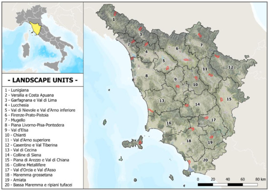
Figure 1.
The 20 study areas (in red) selected for each landscape unit identified by the regional Landscape Plan.
- Hydro-geomorphological systems;
- Eco-systemic characters;
- The long-term configuration of the settlements and of the infrastructures;
- The characters of the rural territory;
- The perception of the territory;
- The sense of belonging of the communities;
- The local socio-economic systems;
- The settlement dynamics and the forms of intercommunality.
In the Landscape Plan logic, landscape units are therefore homogeneous areas for what concern the geomorphological characteristics, the features and values of the rural landscape and the socio-economic system. For the definition of the landscape units, in order to increase the territorial policies’ effectiveness and in respect of the sense of belonging of the local communities, the municipal borders were generally used as boundaries.
The first phase of the project was the identification of a representative area for each landscape unit, according to the information reported in their description inside the plan. After the 20 monitoring areas’ identification (Figure 1, Table 1), the boundaries were shaped using well-recognizable territorial features, such as roads, ridges and rivers. It was decided to realize monitoring areas with a surface established in 1000 hectares to make the results easily comparable between the different areas. The choice of this surface was made because it is large enough to be considered representative of the landscape features of the area and, at the same time, it is contained in order to allow a very high level of detail regarding the land uses and the landscape structure. Moreover, a surface that is not too large allows an update of the periodic monitoring in short times.

Table 1.
Landscape units, municipalities and coordinates of the central point for all the 20 selected study areas.
The boundaries of the monitoring areas were identified and shaped through the open source GIS software Quantum GIS, using as a cartographic base the Regional Technical Map (CTR) 1:10,000 and the 2016 orthophoto with resolution equal to 20 cm. These cartographic sources are freely consultable through Geoscopio, the official Web Map Service (WMS) of the Tuscan region.
2.2. The Methodology
After the study areas selection, land use mapping through video-based photo interpretation was carried out. This part of the study was conducted with Quantum GIS software and with 20 cm-resolution 2016 orthophotos available through the WMS of the Tuscany region. Due to the high resolution of the orthophotos, it was possible to obtain detailed land use maps, with a minimum cartographic unit of 500 m2, in order to detect all the characteristics of the analyzed landscape and the structure of its mosaic. Some standard parameters were applied for the delimitation of roads or for woods. Roads were considered as polygons if the width was greater than 10 m, while woods were classified as such if the surface was greater than 2000 m2 and the width greater than 20 m. The legend was designed to effectively describe the great variety of land uses in the regional territory. Beside land uses, also the presence of protected areas of different types was evaluated for each study area: national parks, regional natural parks, regional natural reserves, Natura 2000 sites, RAMSAR, Protected Areas of Local Interest (ANPIL).
The third step was the analysis of the landscape structure through the application of some synthetic indexes that provide information on the level of complexity of the mosaic, on fragmentation and, in general, on its structure (Table 2). Cultural landscape-focused research is, in fact, commonly based on the evaluation of two different aspects: the land use system and the landscape mosaic structure, as land use and cover are considered primary factors affecting ecosystems [28,34,35,36,37]. Starting from the 1990s, the use of landscape metrics became common in landscape ecology-related studies [38,39], as the quantification of spatial heterogeneity helped in correlating ecological processes and spatial patterns. The use of different state indicators is, in fact, useful to describe in a synthetic way the main characteristics of the landscape structure [40]. Despite the fact that a great variety of landscape metrics have been developed over the last thirty years [41], it is important to choose the metrics to be applied in order to properly describe the landscape characteristics according to the aim of the research. The choice of the indexes used in our research was carefully evaluated, analyzing previous review studies, especially the ones that related the use of landscape metrics to landscape planning [39,41,42,43,44,45]. The choice of the indexes was also based on the fact that the proposed methodology was developed also with the aim of providing a simple methodology easily replicable in other cultural landscapes, both in in Italy and abroad, as a support to territorial and landscape planning and monitoring. The use of the selected indexes, which, at the same time, are limited in number and easy to calculate, allows this methodology to be replicated with reduced costs for the organizations in charge of landscape planning, which, in this way, could take advantage of a standard methodology to monitor over time and space the effects of its landscape policies, and therefore to adjust them to the situation. Therefore, it was decided to use the following landscape metrics: number of land uses, number of patches (NP), mean patch size (MPS), Hill’s diversity number, edge density (ED).
Table 2.
Description of the applied landscape metrics [47,48].
After that, a 1-hectare hexagon grid was realized using Quantum GIS with the MMQGIS plug-in, for all of the region. Only the hexagons overlapping the study areas were selected and extracted to perform the following analysis. For each hexagon, the number of patches totally or partially included and the variety of land uses (number of different land uses) were measured. Therefore, this tessellation of the study areas allowed calculating two further indexes: patch density (PD) and land use diversity (LUD). These metrics are expressed as the number of patches per hectare and the number of different land uses per hectare, respectively, allowing representing the complexity of the landscape on a map for each study area. The results were then shown using a bivariate legend, creating one map for each study area, and further analyzed to investigate the landscape mosaic structure according to the different typologies of the prevailing landscape. Finally, the data regarding the PD and the LUD for each hexagon and for each study area were elaborated with the IBM SPSS Statistics 27 software to produce the graphs.
The use of hexagons to carry out regular tessellations for landscape structure analysis is due to the fact that this kind of grid can offer different advantages: any given point inside a hexagon is closer to the center of that hexagon than any given point in an equal-area square or triangle would be, and hexagons are the only geometric shape for regular tessellations that shares a real border with every neighbor [46]. To achieve homogenous spatial units for proper statistical analysis, we produced a hexagon grid and clipped samples from the land cover dataset. Since changes in the extent of the hexagons can produce unpredictable behavior of landscape metrics, we tested two different grids (1 ha, 3 ha), finding that the grid of 1-ha hexagons guaranteed a representative sample of patches and of the land uses number per hexagon for our study areas.
3. Results
Data on land uses were merged into three macro-categories (cultivations, forests, built-up areas), in order to make the comparison between the 20 study areas more immediate and to identify the main landscape typology for each area (Figure 2). Results are presented according to the main landscape typology identified, while Table 3 reports all the metrics, and Figure 3 shows all the landscape complexity maps of the 20 study areas with the patch density and land use diversity for each hexagon.
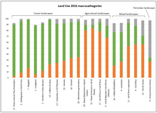
Figure 2.
Percentage of the main land use macro-categories for 2016 for each study area: forests and shrublands (green), agricultural areas (orange) and built-up areas (gray).
Table 3.
Land use macro-categories’ percentages, percentage of protected surface and the different landscape structure indexes calculated for the 20 study areas.
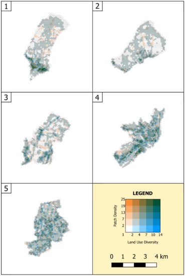
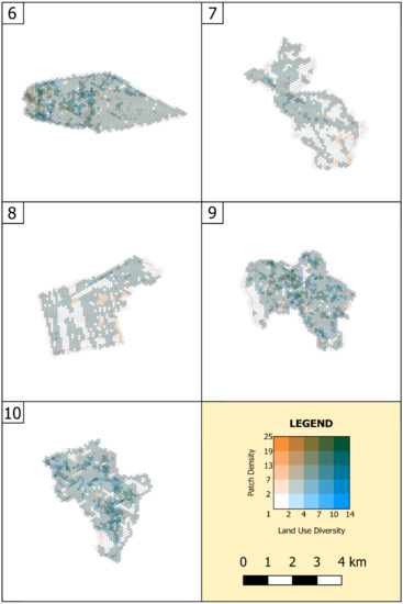
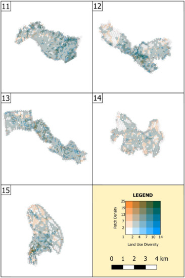
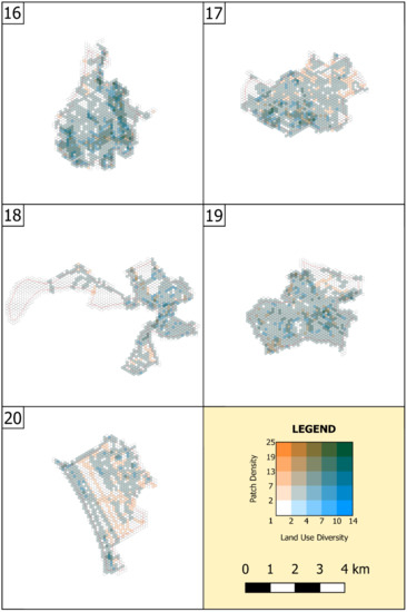
Figure 3.
Maps of the 20 study areas with the patch density and land use diversity for each hexagon. The bivariate legend shows the two different index intensities per hexagon, and thus the landscape complexity distribution.
3.1. Forest Landscapes
The study areas where forests are located on more than 60% of the total surface are ten. Among these, the Plain of Pisa-Livorno-Pontedera (LU8) stands out with 87% of wooded areas, as it is located within the natural parks of Migliarino and San Rossore. Despite the fact that coastal pine forests represent a typical landscape of the area, they do not exhaustively describe a very heterogeneous LU, in which urban sprawl, in recent decades, has affected a considerable surface. Except in two areas (Garfagnana and Val di Lima (LU3), Maremma grossetana (LU18)), the study areas included in this typology are always affected by different types of protected areas. Regarding the number of land uses and Hill’s diversity number, medium-low values are found, a sign that mainly forest landscapes are dominated by a small number of land uses. With regard to the MPS, the values are very dissimilar, sometimes presenting very large patches, particularly in the Plain of Livorno-Pisa-Pontedera (LU8) (6.13 ha), while in the case of Casentino and Val Tiberina (LU12), the average value is less than 1 ha. This is mainly due to the fact that in some study areas, traditional agricultural activities are still carried out, contributing to lowering the value of the average surface. The trend, however, is to have a medium-wide-grained structure due to the homogeneity and continuity of forest surfaces, with the resulting reduced landscape diversity, also as a consequence of the increase in forest areas occurring in recent decades. The values of the ED reflect this issue: from 799 in the Hills of Siena (LU14) to over 2150 in Lunigiana (LU1). The prevalent types of woods are those with a prevalence of chestnut and a prevalence of deciduous oaks. Additionally, noteworthy is the presence of chestnut groves, formations of a high landscape, historical-cultural and biodiversity importance, often with monumental plants; the chestnut groves, in regression throughout the Apennines, were identified mainly in the study areas Amiata (LU19) and Mugello (LU7), where, in fact, chestnuts are considered a typical product. Finally, in the case of the study area Lucchesia (LU4), there are numerous Robinia pseudoacacia woods. By analyzing PD and LUD data (Figure 4a,b), forest areas show numerous outliers. This situation is the result of the spatial distribution of anthropogenic activities, since most of the area is covered by large forest tiles, while other activities—agricultural ones—are carried out in small and concentrated areas. As a result, most of the hexagonal tiles are occupied by few land uses, while only in a few of them—the outliers—are numerous land uses found.
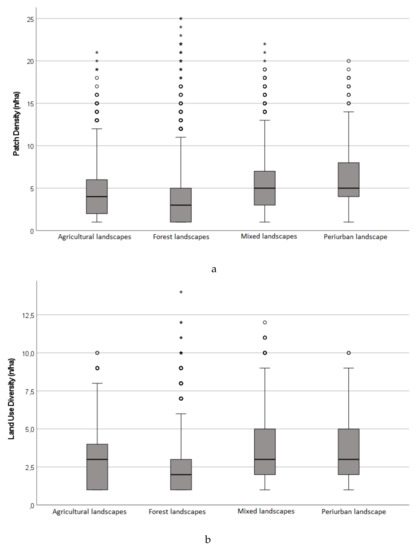
Figure 4.
Results of the patch density (a) and of the land use diversity (b) calculated for each study area based on the 1-hectare hexagonal grid, according to the prevailing landscape typology.
3.2. Agricultural Landscapes
The study areas occupied mainly by agricultural landscapes (agricultural area > 60% of the total surface) total four, with the maximum coverage of these land uses in the Plain of Arezzo and Val di Chiana (LU15) exceeding 84%. Only one of these areas is affected by protected areas, the Val d’Orcia and Val d’Asso (LU17), almost entirely included in the ANPIL Val d’Orcia. Regarding the number of land uses, there is a large difference between the total number of identified land uses and Hill’s diversity number. This fact is attributable to the spread of wide specialized monocultures, especially of olive trees and vines, that dominate the agricultural landscape, despite the fact that there are still many sparse and small patches that preserve traditional agricultural typologies, such as mixed crops or associations between olive trees and vines. This is the case of the Lower Maremma (LU20), dominated by simple arable land, where the MPS is very high (2.96 ha) and Hill’s diversity number is very low (4.8) compared to the total number of land uses (28). ED values of this landscape typology are generally low, a sign that the level of complexity of the landscape mosaic is low, with a landscape dominated mainly by patches of a regular shape, typical of arable crops. The simplification of the agricultural network and the expansion of monocultures, a phenomenon particularly identifiable in these study areas, have greatly changed the structure of the landscape mosaic, even if traditional land uses are still present. The situation regarding the MPS and, in general, the landscape mosaic structure is instead very diversified, as highlighted by the PD and LUD elaborations (Figure 4a,b), with wider interquartile ranges and min–max distance. The study area Val di Nievole and lower Val d’Arno (LU5) has one of the lower MPSs (0.52 ha) due to the presence of specialized cultivations (arable land and vineyards) but on small patches, probably due to the parcelization of the properties, resulting in a diversified landscape. In other study areas, the situation is heterogeneous, as there are large arable land fields in the valley floors, while slopes are balanced by the presence of small olive groves on the slopes. In Val d’Orcia and Val d’Asso (LU17), the forest component of the landscape takes on a more incisive role (about 16% of the total surface), which, in combination with an abundant presence of arable land and vineyards with medium-small tiles, slightly reduces the complexity of the landscape, with an MPS of 1.17 ha. By comparing the data related only to the vineyards of this area to the ones of Chianti (LU10), which, despite being predominantly wooded, is also crucial for wine production, it is possible to notice that the average surfaces of the vineyards for LU17 and LU10 are 0.79 and 1.32 ha, respectively. Chianti (LU10) is, in fact, characterized by a dense and complex landscape mosaic, essentially due to the presence of dry stone terraces, a particular feature of the area, which allow traditional agriculture to be maintained. The study area of Val d’Orcia and Val d’Asso (LU17), on the other hand, presents a landscape mosaic with a medium-large grain, where the cultivation of vines has been favored by the extensive and gentle hills that allow a superficial expansion of this crop, unlike the Chianti study area, whose slopes are steeper and, therefore, do not allow an intensive cultivation of vineyards. The data analyses about the PD and LUD show that the agricultural landscapes are characterized by a significantly higher PD than forest landscapes, while the LUD is similar. This is because, while in an agricultural system, the patches are usually smaller than in a forest system—and therefore the number of patches per hexagon increases—the land uses are rather similar, for example, in the case of numerous fields that share the same land use. Anthropic activities in these areas are also more dispersed throughout the territory, reducing the number of outliers. The interquartile is still wider than the forest landscapes because the wood patches are way more homogeneous and larger than the cultivated areas.
3.3. Mixed Landscapes
Five study areas are characterized by mixed landscape, where no macro-category exceeds 60% of the surface, with a substantial balance between forests and agricultural areas. In three cases, agricultural areas cover more than half of the surface, while in Lucchesia (LU4) and in the Metalliferous Hills (LU16), it is the forest areas that cover more than half of the surface (from 50% to 57%). Val d’Elsa (LU9), Upper Val d’Arno (LU11) and Val di Cecina (LU13) have an agricultural area between 53% and 57%, with small tiles that form a fine-grained agricultural landscape. The forests present in LU9 and LU11 are fragmented, mainly made of small forest surfaces interspersed with agricultural ones, forming a landscape characterized by an interesting mosaic of cultivations on small-medium patches surrounded by forests; in Val di Cecina (LU13), woods are mainly made up of coastal pine forests and small regional forest reserves in the hinterland. The study area Val di Cecina (LU13) is also characterized by diffused anthropized areas along the coast, due to the spread of the touristic hamlet of Donoratico. The values of the indexes of these five areas are particularly heterogeneous. The number of land uses varies from 27 in Val d’Elsa (LU9) to 46 in Val di Cecina (LU13), while Hill’s diversity number values are medium-high, with a particular peak in the Val d Cecina (LU13) area reaching 17.1. The MPS is between 0.5 and 0.79 ha, a sign of a very fragmented mosaic, also due to the presence of numerous land use categories which increases the complexity and diversity of the landscape, but with predominantly regular-shaped tesserae, as evidenced by the ED values. Mixed and periurban landscapes show similar PD and LUD values; although the first ones are found to have a lower inter-quantile PD than the second ones, the median value is the same. The greater complexity of these landscapes is thus evident from these analyses as well, and the intertwining of forest and agricultural areas leads to higher PD and LUD values.
3.4. Periurban Landscapes
The situation of the study area Florence-Prato-Pistoia (LU6) is particular, since it is an area with a predominantly urbanized landscape. Given the characteristics of this landscape unit, the choice of the study area appears highly representative of the landscape dynamics and of the critical issues affecting periurban landscapes. Despite the fact that this area is mainly urbanized, there still are numerous vegetable gardens, family orchards and small cultivated areas, often with traditional crops, as testified by the number of land uses and by the MPS. These cultivated plots, although small in terms of overall surface, are very important for various reasons (agrobiodiversity, landscape, historical-cultural, social, ecological). This situation is also confirmed by the PD and LUD elaborations (Figure 4a,b), especially by the fact that the interquartile range is more compact and is located in the lower part of the graphs, but at the same time, there is a high number of outliers reaching high values.
4. Discussion
The methodology applied in this study was chosen due to the need for assessing and describing different landscape typologies that characterize the Tuscan territory. The use of a hexagonal grid has already been applied with success in other researches to correlate maps, spatial analysis and statistics [49] and proved to be particularly effective for the study of fine-scale Mediterranean landscape mosaics [45,50,51,52]. The applied methodology resulted in being effective in assessing the landscape mosaic structure of different typologies of the landscape in Tuscany and also in creating a database that can represent a crucial baseline for a monitoring system based on fixed study areas that can be easily updated, similarly to what has already been conducted at the national level in Italy [53] and in other European countries [54,55]. The combination of PD and LUD calculated on the basis of the hexagonal grid allows obtaining landscape complexity maps. In fact, according to Plexida et al. [56], there is no need to use too many landscape metrics to properly describe landscape heterogeneity and complexity; some of them, such as patch density, are suitable to describe Mediterranean landscape patterns irrespective of the scale [56], while the MPS provides data about the grain of the landscape [44]. Providing quantitative spatial data related to the different landscape structures through the measurements of appropriate landscape metrics can be extremely useful to transfer the concepts of landscape ecology to sustainable landscape planning and monitoring [42,43,57,58].
Regarding the prevailing landscape typology and the choice of the study areas, it is not surprising that 10 out of 20 areas fall into the forest landscape typology, as more than 50% of the regional surface is covered by forests [59]. In this regard, the choice of the study areas perfectly represents the different main landscape typologies of Tuscany. As highlighted by Slámová et al. [60], investigating the different landscape typologies and their landscape structure and complexity contributes to understanding their multifunctional role. Investigating different landscape structures and complexity is also crucial as they can have different roles for biodiversity [61].
The results highlight a correlation between the landscape typologies and the complexity of the landscape structure, especially in relation to the MPS and the PD. These two indexes, together with other landscape metrics, are considered useful parameters to assess the complexity of the landscape structure of rural areas and are commonly used [62].
According to the MPS, study areas with prevailing mixed landscapes are all fine-grained, with a very complex mosaic made of various land use category alternations, which increases the complexity and diversity of the landscape, a characteristic also common to other Mediterranean countries [63]. The periurban area shows a very fine grain too, due to the presence of vegetable gardens, family orchards and other small cultivated areas that survived the urbanization process. Forested areas are mainly constituted by a landscape structure with a medium-large grain, with a few big forested patches surrounding small cultivated fields near the rural settlements. Agricultural areas have a larger variability, due to the fact that they include both flat and wide cultivated areas in southern Tuscany, as well as small cultivated terraced fields in the hills, as a result of different historical land organization forms. Landscape typologies characterized by a widespread presence of forests are the ones with a lower LUD and a higher PD, and therefore a lower complexity. The reason can also be found in the fact that forests have largely been abandoned by traditional management in the last 70 years. This trend, common in European countries [64], has led to the simplification of forest areas, as the various forest types that were common in the past evolved towards bigger and homogeneous forest patches with lower biodiversity and lower landscape and historical-cultural value.
According to the results of this research, agricultural and especially mixed landscapes are the typologies characterized by higher levels of complexity, as highlighted by the higher number of land uses and of patches per hectare, and by the lower average size of the patches.
On the basis of the results obtained, it is possible to state that the agricultural landscape of Tuscany is dominated by a medium-fine-grain landscape structure, except for the southern part of the region (provinces of Siena and Grosseto) that are characterized by a medium-large-grain landscape structure. International surveys at the European level, such as the Land Use/Cover Area Frame Survey (LUCAS) 2012, propose four different categories of landscape structure fragmentation based on the field size: <0.5 ha, 0.5–1 ha, 1–10 ha and >10 ha [65]. According to our results, the class 1–10 ha is too wide and not appropriate to describe the fragmentation of Southern Europe cultural landscapes, usually characterized by small-scale agriculture [66]. Therefore, we propose the following classification according to the average patch surface for Southern Europe cultural landscapes:
- Small-grain landscape structure: <1 ha;
- Medium-grain landscape structure: 1–2 ha;
- Large-grain landscape structure: >2 ha.
Regarding the presence of protected areas, it is evident that most of the monitoring areas are characterized by an almost complete protection of the surface (five areas have at least 80% of the surface under environmental protection) or no protection at all (nine areas). Few areas have an intermediate situation. The monitoring areas characterized by a high presence of protected areas are often the ones with a higher coverage of forests. Environmental protections have largely been applied in recent decades to forest areas considered more natural, without taking into consideration the fact that in Italy, forests have been regularly managed by man through the centuries. The presence of protected areas, in fact, means that the landscape is associated with “natural values” [67], often without considering the specific history and origin of the actual vegetation. Examples can be found in LU2 and LU8, the first one being historically characterized by chestnut groves and the second one by coastal pine woods planted after land reclamation [68,69]. Both of them largely suffered from abandonment of human activities, and protections have not preserved the characteristic type of forest from evolving towards other types. A large part of the current forest surfaces in Italy, preserved according to national and regional laws, are, for a large part, the result of the abandonment of traditional agro-pastoral practices [70]. This trend is also common to other European countries, even in protected areas [71], and is causing a simplification and homogenization of the rural landscape. As demonstrated by a recent study by Piras et al. [72], 30% of the Tuscan forests currently included in protected areas are the result of secondary successions and most of the total forest area has been shaped by human interventions for what concern species composition and vertical and horizontal structures. This suggests that the protection laws and regulations currently applied are not adequate for preserving these cultural forests as they were developed mainly to protect “natural environments”.
5. Conclusions
Tuscany is a very heterogeneous region in terms of morphology and climate, which is also reflected by a significant diversity of texture. As an accomplice of morphology, it is the human history in this area, as well as in most Mediterranean countries, which has led traditions and customs, sometimes very distant from each other, to modify the territory and, therefore, the landscape and its structure. Assessing the structures of the different landscapes characterizing a region is crucial as they are an integral part of every country’s heritage that significantly contribute to the increase and preservation of biodiversity, landscape diversity and cultural diversity [73].
The evolutionary trends affecting the regional territory are of different types: (i) the abandonment of mountain areas leads to the expansion of forests, typically composed of large and not very diversified patches; (ii) the expansion of fields due to mechanization, which involves the areas in the plains, also leads to an increase in grain size and to a decrease in the overall complexity; (iii) the phenomenon of urbanization, which mainly involves areas previously used for agricultural activities in the plains, that leads to a fragmentation of the landscape mosaic, thanks also to the survival of small vegetable gardens and family orchards.
The main limitation of this research, as well as similar ones, is due to the fact that the choice of the study areas may affect the results. While casual sampling methods, commonly used for forest inventories or similar studies [74], could lead to more objective results and data, in this research this would not have necessarily provided more reliable data, as the sample points should not necessarily be representative of the landscape characteristics of the different LU. For these reasons, we preferred to base the choice of the study areas on the different features of the landscape units as they are described in the Regional Landscape Plan, trying to represent the variability in terms of land uses, morphology and altitude.
Thanks to the results obtained with the present research, it was possible to highlight the characteristics of the structure and complexity of the main Tuscan landscape typologies, providing a crucial baseline for future monitoring and for assessing the effectiveness of planning policies. This turns out to be useful to improve and address planning, management and protection strategies respecting all the local differences, since the awareness of the history and of the current landscapes’ features is not just scientifically interesting but can also change our perspective on future planning, management and protection [75]. The most important contribution to the future planning instruments of the Tuscan region comes from the fact that, through this research, it was possible to provide scientific and quantitative data for each landscape unit, as the current Landscape Plan includes detailed descriptions of the characteristics and of the vulnerabilities of the different landscape units, but without any data or measurement. This will allow updating and adjusting the planning and protection strategies according to the results of this research and the expected future steps. In fact, as already stated, it is planned to set up a complete monitoring of the Tuscan landscape, based on a regular update of the land use maps and of the landscape metrics of the twenty LU, and on analysis of the historical landscape through photo interpretation of past aerophotos. This will allow obtaining a large amount of data in particularly high detail, on the trend and on the current state of this fundamental resource of the regional territory. Finally, the applied methodology can be easily replicated in other contexts characterized by cultural landscapes in Italy or abroad, for planning or monitoring purposes, as it is capable of providing quantitative data about land uses, landscape structure complexity, characteristics and vulnerabilities, without large commitments of time and money for the public bodies in charge of territorial and landscape planning.
Author Contributions
Conceptualization, A.S., M.V. and F.P.; methodology, A.S., F.P., F.C. and B.F.; software, A.S., F.P. and F.C.; writing, A.S., M.V., F.C. and B.F.; supervision, A.S., M.V. and M.A. All authors have read and agreed to the published version of the manuscript.
Funding
This research received no external funding.
Institutional Review Board Statement
Not Applicable.
Informed Consent Statement
Not Applicable.
Data Availability Statement
The data presented in this study are available on request from the corresponding author.
Conflicts of Interest
The authors declare no conflict of interest.
References
- Van der Ploeg, J.D.; Roep, D. Multifunctionality and rural development: The actual situation in Europe. Multifunct. Agric. 2003, 3, 37–54. [Google Scholar]
- Fischer, J.; Meacham, M.; Queiroz, C. A plea for multifunctional landscapes. Front. Ecol. Environ. 2017, 15, 59. [Google Scholar] [CrossRef]
- Mouchet, M.; Paracchini, M.; Schulp, C.; Stürck, J.; Verkerk, P.; Verburg, P.; Lavorel, S. Bundles of ecosystem (dis)services and multifunctionality across European landscapes. Ecol. Indic. 2017, 73, 23–28. [Google Scholar] [CrossRef]
- European Commission. Our Life Insurance, Our Natural Capital: An EU Biodiversity Strategy to 2020; COM (2011) 244; European Commission: Brussels, Belgium, 2011. [Google Scholar]
- Song, B.; Robinson, G.M.; Bardsley, D.K. Measuring Multifunctional Agricultural Landscapes. Land 2020, 9, 260. [Google Scholar] [CrossRef]
- Angelstam, P. Conservation of Communities—The Importance of Edges, Surroundings and Landscape Mosaic Structure. In Ecological Principles of Nature Conservation; Springer Science and Business Media LLC: Boston, MA, USA, 1992; pp. 9–70. [Google Scholar]
- Assandri, G.; Bogliani, G.; Pedrini, P.; Brambilla, M. Beautiful agricultural landscapes promote cultural ecosystem services and biodiversity conservation. Agric. Ecosyst. Environ. 2018, 256, 200–210. [Google Scholar] [CrossRef]
- Molnár, Z.; Berkes, F. Role of traditional ecological knowledge in linking cultural and natural capital in cultural landscapes. In Reconnecting Natural and Cultural Capital: Contributions from Science and Policy; Paracchini, M.L., Zingari, P.C., Blasi, C., Eds.; Publications Office of the European Union: Luxembourg, 2018; pp. 183–193. [Google Scholar]
- Santoro, A.; Venturi, M.; Ben Maachia, S.; Benyahia, F.; Corrieri, F.; Piras, F.; Agnoletti, M. Agroforestry Heritage Systems as Agrobiodiversity Hotspots. The Case of the Mountain Oases of Tunisia. Sustainability 2020, 12, 4054. [Google Scholar] [CrossRef]
- Scazzosi, L. Rural Landscape as Heritage: Reasons for and Implications of Principles Concerning Rural Landscapes as Herit-age. ICOMOS-IFLA 2017. Built Herit. 2018, 2, 39–52. [Google Scholar] [CrossRef]
- Eriksson, O. What is biological cultural heritage and why should we care about it? An example from Swedish rural land-scapes and forests. Nat. Conserv. 2018, 28, 1–32. [Google Scholar] [CrossRef]
- Rotherham, I.D. Bio-cultural heritage and biodiversity: Emerging paradigms in conservation and planning. Biodivers. Conserv. 2015, 24, 3405–3429. [Google Scholar] [CrossRef]
- Del Lungo, S.; Sabia, C.A.; Pacella, C. Landscape and Cultural Heritage: Best Practices for Planning and Local Development: An Example from Southern Italy. Procedia Soc. Behav. Sci. 2015, 188, 95–102. [Google Scholar] [CrossRef]
- Sooväli, H.; Palang, H.; Külvik, M. The role of rural landscapes in shaping Estonian national identity. European Landscapes: From Mountain to Sea. In Proceedings of the Permanent European Conference for the Study of the Rural Landscape at London and Aberystwyth, Huma, Tallin, Estonia, 10–17 September 2000; pp. 114–121. [Google Scholar]
- Torquati, B.; Tempesta, T.; Vecchiato, D.; Venanzi, S.; Paffarini, C. The value of traditional rural landscape and nature pro-tected areas in tourism demand: A study on agritourists’ preferences. Landsc. Online 2017, 53, 1–18. [Google Scholar] [CrossRef]
- Daugstad, K. Negotiating landscape in rural tourism. Ann. Tour. Res. 2008, 35, 402–426. [Google Scholar] [CrossRef]
- Villanueva-Álvaro, J.J.; Mondéjar-Jiménez, J.; Sáez-Martínez, F.J. Rural tourism: Development, management and sustainability in rural establishments. Sustainability 2017, 9, 818. [Google Scholar] [CrossRef]
- Kneafsey, M. Tourism, Place Identities and Social Relations in the European Rural Periphery. Eur. Urban Reg. Stud. 2000, 7, 35–50. [Google Scholar] [CrossRef]
- Koohafkan, P.; Altieri, M.A. Globally Important Agricultural Heritage Systems. A Legacy for the Future; Food and Agriculture Organization of the United Nations: Rome, Italy, 2011. [Google Scholar]
- Agnoletti, M.; Santoro, A. Rural landscape planning and forest management in Tuscany (Italy). Forests 2018, 9, 473. [Google Scholar] [CrossRef]
- Agnoletti, M. Paesaggio Rurale. Strumenti per la Pianificazione Strategica; Edagricole: Bologna, Italy, 2010. [Google Scholar]
- Randelli, F.; Martellozzo, F. Is rural tourism-induced built-up growth a threat for the sustainability of rural areas? The case study of Tuscany. Land Use Policy 2019, 86, 387–398. [Google Scholar] [CrossRef]
- ISTAT. Le Aziende Agrituristiche in Italia: Rapporto 2015; ISTAT: Rome, Italy, 2016.
- IRPET. Rapporto sul Turismo in Toscana; IRPET: Florence, Italy, 2016. [Google Scholar]
- Decreto Legislativo 22 Gennaio 2004, n. 42. Codice dei Beni Culturali e del Paesaggio. Gazzetta Ufficiale n. 45 del 24 Febbraio 2004, s.o. n. 28. Available online: https://www.camera.it/parlam/leggi/deleghe/testi/04042dl.htm (accessed on 11 May 2021).
- Giunta Regionale Toscana. Legge per il Governo n. 65/2014. Available online: http://raccoltanormativa.consiglio.regione.toscana.it/articolo?urndoc=urn:nir:regione.toscana:legge:2014-11-10;65&pr=idx,0;artic,1;articparziale,0 (accessed on 11 May 2021).
- Council of Europe. The European Landscape Convention; Council of Europe: Strasbourg, France, 2000. [Google Scholar]
- Lausch, A.; Blaschke, T.; Haase, D.; Herzog, F.; Syrbe, R.U.; Tischendorf, L.; Walz, U. Understanding and quantifying land-scape structure—A review on relevant process characteristics, data models and landscape metrics. Ecol. Model. 2015, 295, 31–41. [Google Scholar] [CrossRef]
- Frazier, A.E.; Kedron, P. Landscape Metrics: Past Progress and Future Directions. Curr. Landsc. Ecol. Rep. 2017, 2, 63–72. [Google Scholar] [CrossRef]
- Li, H.; Wu, J. Use and misuse of landscape indices. Landsc. Ecol. 2004, 19, 389–399. [Google Scholar] [CrossRef]
- McGarigal, K.; Tagil, S.; Cushman, S.A. Surface metrics: An alternative to patch metrics for the quantification of landscape structure. Landsc. Ecol. 2009, 24, 433–450. [Google Scholar] [CrossRef]
- Walz, U. Landscape Structure, Landscape Metrics and Biodiversity. Living Rev. Landsc. Res. 2011, 5, 1–35. [Google Scholar] [CrossRef]
- Giunta Regionale Toscana. Piano di Indirizzo Territoriale con valenza di Piano Paesaggistico; Regione Toscana: Florence, Italy, 2015. [Google Scholar]
- Müller, D.; Munroe, D.K. Current and future challenges in land-use science. J. Land Use Sci. 2014, 9, 133–142. [Google Scholar] [CrossRef]
- Verburg, P.H.; van de Steeg, J.; Veldkamp, A.; Willemen, L. From land cover change to land function dynamics: A major challenge to improve land characterization. J. Environ. Manag. 2009, 90, 1327–1335. [Google Scholar] [CrossRef] [PubMed]
- Schaich, H.; Bieling, C.; Plieninger, T. Linking Ecosystem Services with Cultural Landscape Research. GAIA Ecol. Perspect. Sci. Soc. 2010, 19, 269–277. [Google Scholar] [CrossRef]
- Cegielska, K.; Noszczyk, T.; Kukulska, A.; Szylar, M.; Hernik, J.; Dixon-Gough, R.; Jombach, S.; Valánszki, I.; Kovács, K.F. Land use and land cover changes in post-socialist countries: Some observations from Hungary and Poland. Land Use Policy 2018, 78, 1–18. [Google Scholar] [CrossRef]
- Turner, M.G. Spatial and temporal analysis of landscape patterns. Landsc. Ecol. 1990, 4, 21–30. [Google Scholar] [CrossRef]
- Haines-Young, R.; Chopping, M. Quantifying landscape structure: A review of landscape indices and their application to forested landscapes. Prog. Phys. Geogr. Earth Environ. 1996, 20, 418–445. [Google Scholar] [CrossRef]
- Sowińska-Świerkosz, B. Review of cultural heritage indicators related to landscape: Types, categorisation schemes and their usefulness in quality assessment. Ecol. Indic. 2017, 81, 526–542. [Google Scholar] [CrossRef]
- Uuemaa, E.; Antrop, M.; Roosaare, J.; Marja, R.; Mander, U. Landscape Metrics and Indices: An Overview of Their Use in Landscape Research. Living Rev. Landsc. Res. 2009, 3, 1–28. [Google Scholar] [CrossRef]
- Leitão, A.B.; Ahern, J. Applying landscape ecological concepts and metrics in sustainable landscape planning. Landsc. Urban Plan. 2002, 59, 65–93. [Google Scholar] [CrossRef]
- Herzog, F.; Lausch, A. Supplementing land-use statistics with landscape metrics: Some methodological considerations. Environ. Monit. Assess. 2001, 72, 37–50. [Google Scholar] [CrossRef]
- Herzog, F.; Lausch, A. Prospects and limitations of the application of landscape metrics for landscape monitoring. In Heter-ogeneity in Landscape Ecology: Pattern and Scale; Proceedings of the 8th Annual Conference of the International Association of Landscape Ecology, Bristol, UK, 6–8 September 1999; Maudsley, M., Marshall, J., Eds.; IALE: Scotland, UK, 1999; pp. 41–50. [Google Scholar]
- Schindler, S.; Poirazidis, K.; Wrbka, T. Towards a core set of landscape metrics for biodiversity assessments: A case study from Dadia National Park, Greece. Ecol. Indic. 2008, 8, 502–514. [Google Scholar] [CrossRef]
- Adamczyk, J.; Tiede, D. ZonalMetrics—A Python toolbox for zonal landscape structure analysis. Comput. Geosci. 2017, 99, 91–99. [Google Scholar] [CrossRef]
- Hill, M.O. Diversity and Evenness: A Unifying Notation and Its Consequences. Ecology 1973, 54, 427–432. [Google Scholar] [CrossRef]
- Turner, G.M.; Gardner, H.R.; O’Neill, V.R. Landscape Ecology in Theory and Practice; Springer: New York, NY, USA, 2001. [Google Scholar]
- Carr, D.B.; Olsen, A.R.; White, D. Hexagon Mosaic Maps for Display of Univariate and Bivariate Geographical Data. Cartogr. Geogr. Inf. Syst. 1992, 19, 228–236. [Google Scholar] [CrossRef]
- Rusche, K.; Reimer, M.; Stichmann, R. Mapping and Assessing Green Infrastructure Connectivity in European City Regions. Sustainability 2019, 11, 1819. [Google Scholar] [CrossRef]
- Wolff, S.; Lakes, T. Characterising Agricultural Landscapes using Landscape Metrics and Cluster Analysis in Brandenburg, Germany. GI_Forum 2020, 1, 89–98. [Google Scholar] [CrossRef]
- Mirici, M.E.; Satir, O.; Berberoglu, S. Monitoring the Mediterranean type forests and land-use/cover changes using appropri-ate landscape metrics and hybrid classification approach in Eastern Mediterranean of Turkey. Environ. Earth Sci. 2020, 79, 1–17. [Google Scholar]
- Agnoletti, M.; Emanueli, F.; Corrieri, F.; Venturi, M.; Santoro, A. Monitoring Traditional Rural Landscapes. The Case of Italy. Sustainability 2019, 11, 6107. [Google Scholar] [CrossRef]
- Dramstad, W.; Fry, G.; Fjellstad, W.; Skar, B.; Helliksen, W.; Sollund, M.-L.; Tveit, M.; Geelmuyden, A.; Framstad, E. Integrating landscape-based values—Norwegian monitoring of agricultural landscapes. Landsc. Urban Plan. 2001, 57, 257–268. [Google Scholar] [CrossRef]
- Ståhl, G.; Allard, A.; Esseen, P.-A.; Glimskär, A.; Ringvall, A.; Svensson, J.; Sundquist, S.; Christensen, P.; Torell Åsa, G.; Högström, M.; et al. National Inventory of Landscapes in Sweden (NILS)—scope, design, and experiences from establishing a multiscale biodiversity monitoring system. Environ. Monit. Assess. 2010, 173, 579–595. [Google Scholar] [CrossRef] [PubMed]
- Plexida, S.G.; Sfougaris, A.I.; Ispikoudis, I.P.; Papanastasis, V.P. Selecting landscape metrics as indicators of spatial heteroge-neity—A comparison among Greek landscapes. Int. J. Appl. Earth Obs. Geoinf. 2014, 26, 26–35. [Google Scholar] [CrossRef]
- Almenar, J.B.; Bolowich, A.; Elliot, T.; Geneletti, D.; Sonnemann, G.; Rugani, B. Assessing habitat loss, fragmentation and ecological connectivity in Luxembourg to support spatial planning. Landsc. Urban Plan. 2019, 189, 335–351. [Google Scholar] [CrossRef]
- Viana, C.M.; Rocha, J. Evaluating Dominant Land Use/Land Cover Changes and Predicting Future Scenario in a Rural Re-gion Using a Memoryless Stochastic Method. Sustainability 2020, 12, 4332. [Google Scholar] [CrossRef]
- Regione Toscana. Rapporto sullo Stato delle Foreste in Toscana; Regione Toscana e Compagnia delle Foreste S.r.l.: Florence, Italy, 2020. [Google Scholar]
- Slámová, M.; Kruse, A.; Belčáková, I.; Dreer, J. Old but Not Old Fashioned: Agricultural Landscapes as European Heritage and Basis for Sustainable Multifunctional Farming to Earn a Living. Sustainability 2021, 13, 4650. [Google Scholar] [CrossRef]
- Zarnetske, P.L.; Baiser, B.; Strecker, A.; Record, S.; Belmaker, J.; Tuanmu, M.-N. The Interplay Between Landscape Structure and Biotic Interactions. Curr. Landsc. Ecol. Rep. 2017, 2, 12–29. [Google Scholar] [CrossRef]
- Concepción, E.D.; Díaz, M.; Baquero, R.A. Effects of landscape complexity on the ecological effectiveness of agri-environment schemes. Landsc. Ecol. 2008, 23, 135–148. [Google Scholar] [CrossRef]
- Sertel, E.; Topaloğlu, R.H.; Şallı, B.; Algan, I.Y.; Aksu, G.A. Comparison of Landscape Metrics for Three Different Level Land Cover/Land Use Maps. ISPRS Int. J. Geo Inf. 2018, 7, 408. [Google Scholar] [CrossRef]
- FAO; UNEP. The State of the World’s Forests 2020. In Forests, Biodiversity and People; FAO and UNEP: Rome, Italy, 2020. [Google Scholar]
- Tieskens, K.F.; Schulp, C.J.; Levers, C.; Lieskovský, J.; Kuemmerle, T.; Plieninger, T.; Verburg, P.H. Characterizing European cultural landscapes: Accounting for structure, management intensity and value of agricultural and forest landscapes. Land Use Policy 2017, 62, 29–39. [Google Scholar] [CrossRef]
- Van Eetvelde, V.; Antrop, M. Analyzing structural and functional changes of traditional landscapes—two examples from Southern France. Landsc. Urban Plan. 2004, 67, 79–95. [Google Scholar] [CrossRef]
- Solecka, I.; Raszka, B.; Krajewski, P. Landscape analysis for sustainable land use policy: A case study in the municipality of Popielów, Poland. Land Use Policy 2018, 75, 116–126. [Google Scholar] [CrossRef]
- Agnoletti, M. L’Evoluzione del Paesaggio Nella Tenuta di MIGLIARINO fra XIX e XX Secolo; Tipografia Regionale: Florence, Italy, 2005. [Google Scholar]
- Agnoletti, M. Dinamiche del Paesaggio Biodiversità e Rischio Idrogeologico Nella Zona Della Pania di Cardoso Fra 1832 e 2002 (Parco Regionale Delle Alpi Apuane); Tipografia Regionale: Florence, Italy, 2005. [Google Scholar]
- Falcucci, A.; Maiorano, L.; Boitani, L. Changes in land-use/land-cover patterns in Italy and their implications for biodiversity conservation. Landsc. Ecol. 2007, 22, 617–631. [Google Scholar] [CrossRef]
- Oikonomakis, N.G.; Ganatsas, P. Secondary forest succession in Silver birch (Betula pendula Roth) and Scots pine (Pinus syl-vestris L.) southern limits in Europe, in a site of Natura 2000 network—An ecogeographical approach. For. Syst. 2020, 29, 81–96. [Google Scholar]
- Piras, F.; Venturi, M.; Corrieri, F.; Santoro, A.; Agnoletti, M. Forest Surface Changes and Cultural Values: The Forests of Tuscany (Italy) in the Last Century. Forests 2021, 12, 531. [Google Scholar] [CrossRef]
- Bugár, G.; Pucherová, Z.; Veselovská, K. Mosaic Landscape Structures in Relation to the Land Use of Nitra District. Ekológia 2020, 39, 277–288. [Google Scholar] [CrossRef]
- Gasparini, P.; Di Cosmo, L.; Cenni, E.; Pompei, E.; Ferretti, M. Towards the harmonization between National Forest Inventory and Forest Condition Monitoring. Consistency of plot allocation and effect of tree selection methods on sample statistics in Italy. Environ. Monit. Assess. 2012, 185, 6155–6171. [Google Scholar] [CrossRef]
- Renes, H.; Centeri, C.; Kruse, A.; Kučera, Z. The Future of Traditional Landscapes: Discussions and Visions. Land 2019, 8, 98. [Google Scholar] [CrossRef]


Publisher’s Note: MDPI stays neutral with regard to jurisdictional claims in published maps and institutional affiliations. |
© 2021 by the authors. Licensee MDPI, Basel, Switzerland. This article is an open access article distributed under the terms and conditions of the Creative Commons Attribution (CC BY) license (https://creativecommons.org/licenses/by/4.0/).