Abstract
The implementation of ecological projects can largely change regional land use patterns, in turn altering the local hydrological process. Articulating these changes and their effects on ecosystem services, such as water conservation, is critical to understanding the impacts of land use activities and in directing future land planning toward regional sustainable development. Taking Zhangjiakou City of the Yongding River as the study area—a region with implementation of various ecological projects—the impact of land use changes on various hydrological components and water conservation capacity from 2000 to 2015 was simulated based on a soil and water assessment tool model (SWAT). An empirical regression model based on partial least squares was established to explore the contribution of different land use changes on water conservation. With special focus on the forest having the most complex effects on the hydrological process, the impacts of forest type and age on the water conservation capacity are discussed on different scales. Results show that between 2000 and 2015, the area of forest, grassland and cultivated land decreased by 0.05%, 0.98% and 1.64%, respectively, which reduces the regional evapotranspiration (0.48%) and soil water content (0.72%). The increase in settlement area (42.23%) is the main reason for the increase in water yield (14.52%). Most land use covered by vegetation has strong water conservation capacity, and the water conservation capacity of the forest is particularly outstanding. Farmland and settlements tend to have a negative effect on water conservation. The water conservation capacity of forest at all scales decreased significantly with the growth of forest (p < 0.05), while the water conservation capacity of different tree species had no significant difference. For the study area, increasing the forest area will be an effective way to improve the water conservation function, planting evergreen conifers can rapidly improve the regional water conservation capacity, while planting deciduous conifers is of great benefit to long-term sustainable development.
1. Introduction
Since the 21st century, problems related to water resources, such as floods, droughts, and water shortages, have caused increasing problems for human production and life [1,2,3,4]. The conflict between water supply and demand has caused conflicts between national and local strategies [5].
The changes in water resources at the basin scale are significantly affected by climate change and human activities. Compared with the impact of climate on the water cycle and water availability, human activities play an increasingly important role in controlling the water quality and quantity of watersheds [2,6] The impact is mainly reflected in the different land use scenarios formed by changing the land cover types according to people’s needs, and these change the physical and chemical properties of the underlying surface, ultimately affecting hydrological components such as surface runoff [6], interflow [7], soil water content [6], and evapotranspiration [8,9] and threaten the water safety (quality and quantity) of the area. Changes in the proportion of different hydrological components to water expenditure have a direct impact on water conservation capacity. Therefore, analyzing the response of a watershed’s hydrological components to changes in land use is very important for the sustainable development of the watershed, which also actually addresses the interaction between Sustainable Development Goal (SDG) 6 (clean water and sanitation) and SDG 15 (life on land).
The Yongding River is the largest tributary of the Haihe River Basin, and the Guanting Reservoir watershed, upstream of Yongding River, is an important water supply area and ecological barrier in the Beijing–Tianjin–Hebei coordinated development zone. In its upstream, Shanxi and Hebei provinces are major industrial raw material production provinces [10,11], and in its downstream, Beijing’s settlement area expansion and growth of population are rapid. Furthermore, the imbalance between water supply and demand is increasing, and such human activities have increased this imbalance [12,13]. Zhangjiakou City in the watershed is located in the semi-arid and semi-humid transitional zone between Mongolian Plateau and the North China Plain, and sandstorms often have occurred in the Beijing–Tianjin area in the last century. Since 2000, the development of many afforestation ecological projects, such as returning farmland to forests and the Three North Shelterbelt Forest Project, have led to a drastic change in the regional land use [14]. Therefore, exploring the response of hydrological processes to changes in land use and the resulting changes in regional water conservation capacity is very important for the sustainable use of water resources.
The ecological processes and patterns are heterogeneous and complex in spatial distribution. There is heterogeneity among different land use. A distributed hydrological model that can explain spatial heterogeneity has higher accuracy in describing the impact of changes in land use distribution on hydrological processes [15]. The soil and water assessment tool (SWAT) model can dynamically adjust input parameters such as land use types and management operations, making it widely used in the work of evaluating the impact of changes in land use on the hydrological process of the watershed. Many studies have used the SWAT model to evaluate the hydrological effects of land use change. The main research has centered around watershed runoff simulation under different land cover conditions [16,17,18,19], effects of different land cover conditions on watershed water balance [20,21], and source pollution simulation and control under different land cover conditions [22,23,24,25]. Partial least squares (PLSR) is an appropriate method for evaluating hydrological effects of changes in land use. PLSR combines the functions of principal component analysis and multiple linear regression (MLR) [26,27]. When the predictors are highly correlated, PLSR has an accuracy advantage over standard MLR, and this can solve the problem of multicollinearity caused by the mutual conversion between different land uses.
Forest vegetation is an important part of the natural environment. Studies have shown that with the conversion of other land cover types into forests, annual surface runoff will decrease [28] and that regional soil interflow and base flow will have sustained growth [29]. The conversion of land cover types to forests upstream can reduce the downstream risk of flood disasters [30]. The uneven spatial distribution of the forest age structure is an important reason for the heterogeneity of the vertical structure of the forest [31]. Forest age changes the proportion of different components of the canopy, affecting its hydrological processes [32]. For example, the leaf area index changes with forest age and impacts the interception rate [33] and further influences evaporation and runoff. Studying the hydrological effects of forest age will help to explore the impact of regional hydrological composition changes on water conservation capacity. However, most of the studies on the hydrological effects of forest age are based on site survey data, and the spatial representation does not sufficiently reflect the impact of changes in hydrological composition on regional water conservation capacity. In addition, those studies on a large spatial scale rarely paid attention to the hydrological effects of different forest types and forest ages. Therefore, the objectives of this study are as follows. (1) Clarify the impact of long-term land use changes on various hydrological components affecting water conservation in the Zhangjiakou region of the Guanting Reservoir basin. (2) Explore the impact of different forest types and forest age on water conservation capacity on a larger spatial scale. This work provides a certain reference for formulating schemes to deal with water shortages and eventually achieve sustainable development of the basin.
2. Study Area and Data Collection
2.1. Study Area
The Yongding River is the largest tributary of the Haihe River Basin. The river flows through Shanxi Province, the Inner Mongolia Autonomous Region, Hebei Province, then flows to Beijing and Tianjin, and finally flows into the Bohai Sea. Most of the large-scale floods before the 20th century were caused by large-scale deforestation upstream of the Yongding River [34]. To reduce flooding, various water conservancy facilities were built in the basin, and the Guanting Reservoir built in 1954 is one of them. Guanting Reservoir is located in Guanting Village, Huailai County, Hebei Province, about 90 km northwest of Beijing. The Guanting Reservoir watershed belongs to the Yongding River system. There are three major rivers in the basin, Yanghe River, Sanggan River, and Guishui River, with a total area of 4,250,000 ha. The elevation in the basin is 222–2840 m. Zhangjiakou is located upstream of the Yongding River (113°50′–116°30′ E, 39°30′–42°10′ N) and is adjacent to Beijing in the southeast. This area has a continental monsoon climate in East Asia with an average annual temperature of 7.6 °C and annual precipitation of 330–400 mm, which means it is semi-arid.
Because the boundaries of watershed and administrative district are different, the sub-basins in the overlap area of administrative boundary and the watershed forms the study area (Figure 1). This operation maintains the characteristics of the dramatic changes in the land use of Zhangjiakou and quantifies the regional hydrological process without interrupting the boundaries of the catchment.
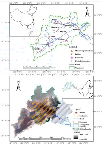
Figure 1.
Location and Digital Elevation Model (DEM) of the Guanting Reservoir watershed. The overlapping area of the Zhangjiakou administrative area and the watershed is the study area. The specific scope is determined by the intersect operation of the sub-watershed and research area.
2.2. Data Collection and Prepare
The input data of this study are meteorological data, hydrological data, and spatial data. Spatial data comprise terrain data, land use data, and soil type data.
Meteorological data are obtained from daily data sets of eight national weather stations provided by the National Meteorological Information Center; these data include average temperature, precipitation, average wind speed, relative humidity, and sunshine hours per day. Discharge data were obtained from the “Hydronomic Yearbook of the People’s Republic of China”. Table 1 shows location information of weather stations, hydrological stations, and reservoirs used in this study.

Table 1.
Location information of weather stations, hydrological stations, and reservoirs used in this study.
The topographic data are 90 m resolution Shuttle Radar Topography Mission (SRTM) DEM data provided by China Geospatial Data Cloud, and the real river network data was introduced to assist the generation of river channels in the watershed.
The distribution of land use was generated by China’s 1:250,000 land cover data produced by the Aerospace Information Research Institute, Chinese Academy of Sciences, and reclassified according to the SWAT land use input code (Figure 2). After reclassification, it mainly includes six land use types, namely, forest, grassland, farmland, settlement, waterbody, and barren land. Under each type, there are several sub-types, among which, forest is divided into four types: evergreen forest (FRSE), deciduous forest (FRSD), mixed forest (FRST), and shrubland (RNGB). Grassland is further divided into meadow grassland (PAST) and shrub grassland (RNGE); farmland (AGRL) is not divided into sub-types; settlements is divided into urban construction land (URHD) and rural settlements (URLD); waterbody is divided into wetlands (WETL) and water (WATR); and barren land (BARR) is not divided into sub-types.
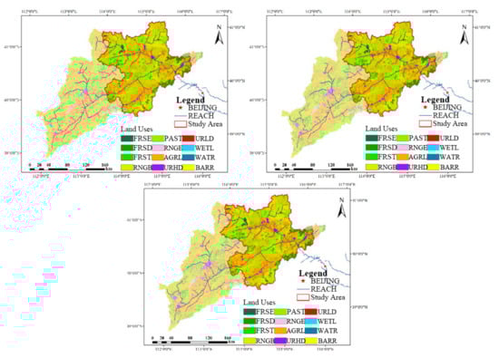
Figure 2.
The distribution of land use types in Guanting Reservoir watershed of 2000, 2010, and 2015 (from top left to bottom right), where the red frame is the research area and the translucent part is the remaining area of the Guanting Reservoir watershed.
Soil data (Figure 3) were obtained from the World Homogeneous Soil Database (HWSD) published by the International Food and Agriculture Organization, which provides a global soil-type distribution map with a resolution of 1 km and a database of different soil textures.
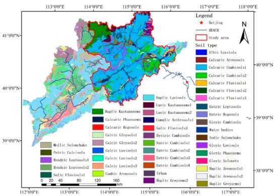
Figure 3.
The distribution soil types in the Guanting Reservoir watershed in 2015, where the red frame is the research area and the translucent part is the remaining area of the Guanting Reservoir watershed.
All input spatial data were processed into a uniform geographic coordinate and projection format to meet the requirements of the SWAT simulation using the WGS84-Albers projection.
3. Methodologies
This study was mainly conducted by the following three parts (Figure 4): (1) Based on the datasets described in Section 2.2, the SWAT model for the Guanting Reservoir watershed was built and used to reconstruct the runoff for the following application. (2) The calibrated SWAT model was used to clarify the contribution of land use change impacts on various hydrological components. (3) Aiming at the forest that has a greater impact on water conservation, the impact of its internal structure differences on water conservation capacity is analyzed.
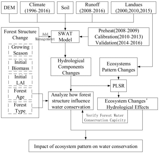
Figure 4.
Technical route.
3.1. SWAT Model
SWAT is a semi-distributed watershed scale model developed by the United States Department of Agriculture Agricultural Research Service. Its development purpose is to predict the impact of different land management schemes on the production of water, sediment, and agrochemicals in large and complex watersheds. The model divided the watershed into sub-basins and hydrologic response units (HRUs). Each HRU represents a unique combination of land use, soil type, and terrain condition, thus forming many different types of land uses. HRU is the basic unit to simulate the hydrological components, nutrients, and sediment production of each sub-basin and then connect them to the entire river network. The river network connects the emissions generated by the sub-basin according to the water balance equation and finally flows to the outlet of the catchment. The daily water balance equation used in the model is the following:
where (mm) is the final soil water content on day t, (mm) is the initial soil water content of the day before day t, (mm) is the precipitation amount on day i, (mm) is the amount of surface runoff on day i, (mm) is the evapotranspiration (ET) amount on day i, (mm) is the amount of water entering the vadose zone from the soil profile on day i, and (mm) is the amount of return flow on day i.
3.2. Parameter Sensitivity Analysis and Calibration
The SWAT model has many input parameters, and each parameter is greatly affected by spatial heterogeneity. Screening the sensitive parameters of different sub-basins through sensitivity analysis can reduce the workload of parameter calibration. In this study, 26 parameters affecting surface runoff, groundwater recharge, and soil water transport were selected, and the uncertainty and sensitivity of the parameters were analyzed by the SWAT calibration and uncertainty program (SWAT-CUP). Parameters’ initial ranges were determined according to the “Absolute SWAT Value” file provided by SWAT. The Latin hypercube sampling (LH-OAT) method was used for calibration, the sequential uncertainty fitting (SUFI-2) program was used to evaluate the sensitivity of the parameters, and the t value and p-value were used as sensitivity evaluation indexes. The t value is the coefficient of the parameter divided by its standard error, and a larger value indicates greater sensitivity. The p-value determines the significance of sensitivity, and a p-value closer to 0 indicates greater sensitivity. According to the results of the sensitivity analysis of the parameters, the following parameters (Table 2) were finally selected for calibration.
Table 2.
List of sensitive parameters and their ranges and fitted values.
In this study, the SWAT model was calibrated and verified in monthly steps. The warm-up period was set from 2008 to 2009, the calibration period from 2010 to 2013, and the verification period from 2014 to 2016. To evaluate the error between simulated values and observed values introduced by the input data or the initial database of the model, the applicability of the model was verified by comparing graphs and statistical standards. The Nash efficiency coefficient (NSE) [35] and goodness of fit (R2) are commonly used indicators to evaluate the fitting effect of the model. The calculation method of the two indicators are as follows:
where and are the observed and simulated values, respectively; and and are the average of the observed and simulated values, respectively. R2 describes the degree of deviation between the simulation results of the model and the measured results. Its value is between 0 and 1 and a larger value indicates better simulation; it is generally believed that a value of approximately 0.5 means an acceptable simulation result [36]. For the simulation of monthly step size, when 0.75 < NSE ≤ 1, the fitting effect is very good; when 0.65 < NSE ≤ 0.75, the fitting effect is good; when 0.50 < NSE ≤ 0.65, the fitting effect is satisfactory; and when 0.50 ≤ NSE, the fitting is not acceptable [37].
3.3. Evaluation Method for Hydrological Effects of Changes in Land Use
The meteorological data from 2008 to 2016 and the land use types in 2015 were used to establish a model and calibrate the parameters. After obtaining the optimal parameters and bringing them back to the model and running the simulation, the year with the best simulation effect was then chosen to analyze the contribution of different land uses to evapotranspiration, soil water content, surface runoff, soil interflow, base flow, and total runoff. Next, the meteorological data of the year with the best simulation used in the presented analysis and the land use of different years were selected as input data of the model, and the simulation results were used for subsequent analysis. Water body and barren land were not included in this study because of their small proportion in the study area.
The hydrological process under natural scenarios is jointly affected by changes in land use and climate (especially precipitation) change. The runoff coefficient can reflect the complex impact of different land uses on regional water resources in a given watershed. It is defined as the ratio of total runoff to total rainfall. This calculation method greatly weakens the impact of precipitation on the hydrological process. Referring to the runoff coefficient algorithm and previous researchers’ calculation method for water conservation [38], this study calculated the surface runoff coefficient and water conservation coefficient and analyzed the hydrological effects of changes in the land use from the perspective of water conservation. The calculation method of the two indicators is as follows:
where CSURQ and CWC represent the surface runoff coefficient and water conservation coefficient, respectively. SURQ, LATQ, GWQ, and PRECIP represent the surface runoff, interflow, base flow, and precipitation, respectively.
In this study, the percentage of the main land uses in each sub-basin of the study area in 2000, 2010, and 2015 was used as the predictor variable; the surface runoff coefficient and water conservation coefficient of each sub-basin calculated from the model simulation values were used as response variables, and the PLSR model was established. Then, we quantitatively analyzed the hydrological effects of land use changes. The general formula can be expressed as follows:
where Xi and Y are the area percentages of different land uses and different hydrological component evaluation indicators in different years, m is the variable in regression, bi is the regression coefficient, and b0 is the constant in regression.
The model building was divided into three parts. First, two land uses were chosen for modeling. Then, for the two different hydrological coefficients mentioned, the land uses that have a great impact on each hydrological coefficient for model establishment were selected. Finally, a model that includes all land uses was built. The standardized regression coefficients in the modeling results eliminate the influence of the dimension of the dependent variable and the independent variable and can be directly used to compare the direction and strength of the relationship between the predictor variable and the response variable. Then, the effects of simultaneous changes in land uses on the regional water conservation capacity were compared.
3.4. Analysis of the Hydrological Effects of Forest Structure Changes
The internal structure of the forest is complex, and the hydrological processes of different forest types and ages are quite different. To explore the changes in regional hydrological processes and the final impact on the water conservation capacity, this study used the scenario simulation method to analyze the potential hydrological effects of forest age and forest type. Keeping meteorological elements, land uses, soil conditions, and topographic elements unchanged, this work simulated a scenario similar to returning farmland to forest by adding plant operations to farmland in a sub-basin of the study area’s upstream area in the year with the best simulation under the 2015 land use. According to the field research information, the annual growing season was set from March 20 to October 25 (the average temperature reaches 5 °C), and 500 trees were planted per hectare. The age group spans from young forest to mature forest (5–70 years) [39], and the hydrological effects of the forest age of different forest types every 5 years on different spatial scales were studied. The leaf area index and biomass at the beginning of the growing season were set according to the age of the forest, and other parameters adopted the default values of the model. Because SWAT assumes the same precipitation in the same sub-basin, the water conservation capacity is expressed by the sum of soil water content, interflow, and base flow.
The main afforestation tree species in the study area are Larix principis and Pinus tabulaeformis. For deciduous conifer represented by Larch, the initial leaf area index was set to 0. For evergreen conifer represented by Chinese pine, the initial leaf area index was the leaf area index at the end of the previous year. The initial biomass was set according to the biomass equation [40], the diameter at breast height and tree height corresponding to the age in biomass equations were determined by the Richard equation [41,42]. The specific calculation method is as follows:
where and denote the diameter (cm) and height (m), respectively; subscripts E and D stand for evergreen conifers and deciduous conifers, respectively; T stands for forest age; W denotes biomass (kg); a is the coefficient related to the density of trees; b is the coefficient related to the growth environment; and the specific values of the equation coefficients are shown in Table 3.
Table 3.
Parameters of biomass equations for different forest types.
4. Results
4.1. Model Calibration
The results of the calibration are shown in Figure 5. We take Yanchi station, a hydrological station located downstream of Guanting Reservoir, as the final water outlet of the study area. The simulation results of Yanchi satisfying with R2 of 0.82 and NSE of 0.52, respectively.
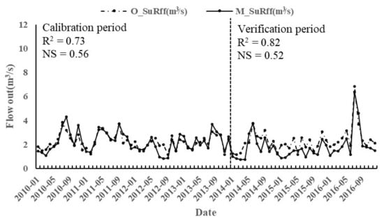
Figure 5.
Simulated (M_SuRff) and observed (O_SuRff) monthly runoff at Yanchi station.
Moreover, the simulation result is better in 2013 with R2 of 0.77, so when analyzing the relationship between land use and water balance components and the hydrological effects of forest structure changes later, simulation results of 2013 were chosen.
4.2. Statistical Characteristics of the Hydrological Components in Different Land Uses
The statistical result of simulation was shown in Figure 6. Except for settlements, the total runoff of the other four land uses was similar, fluctuating between 30 and 40 mm. Wetland had the largest total runoff (39.48 mm) but was much smaller than that of the settlements (88.74 mm). The surface runoff of farmland was greater than that of the other three land uses, while the surface runoff of settlements was 6.94 times larger than that of farmland and accounted for 90.51% of its total runoff.
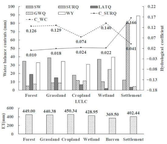
Figure 6.
Hydrological contents of different land use types in the Guanting Reservoir Basin. P denotes precipitation. C_SURQ and C_WC denote surface runoff coefficient and water conservation coefficient, respectively. SW, SURQ, LATQ, GWQ, and WY represent soil water content, surface runoff, interflow, base flow, and total runoff, respectively.
Subsurface runoff (lateral flow + base flow) of forests, grasslands, farmlands, and wetlands had opposite characteristics compared with surface runoff. The subsurface runoff in forests and wetlands was higher, at 26.37 and 26.87 mm, followed by grassland (23.79 mm). The subsurface runoff of farmland was lowest (17.88 mm), while the subsurface runoff of settlements was only 44.35% of that of farmland. In four land uses except for settlements, the sorting of interflow was opposite to that of base flow, which is related to the terrain conditions of different land uses.
Grassland had the highest soil water content (38.85 mm), followed by wetland (37.06 mm) and forest (34.73 mm), while the farmland’s soil water content (18.05 mm) was only 46.47% of that of grassland. The evapotranspiration of different land uses is relatively close, but the evapotranspiration of farmland is the largest, and the evapotranspiration of settlements is the smallest. Compared with farmland, forests and grasslands have less evapotranspiration and surface runoff and more subsurface runoff and soil water content, indicating that both can retain more precipitation.
4.3. Hydrological Effects of Land Use Changes
Table 4 shows the changes in hydrological components and land use areas from 2000 to 2015. The soil water content in the study area has decreased by 0.72% since 2000, and the decrease rate in 2010–2015 has an increasing trend compared with 2000–2010. The grassland area with the highest soil water content has been shrinking, shrinking by 0.99% from 2000 to 2015, and the forest area increasing first and then decreasing is the possible reason for the accelerated soil water content decrease. In 2000, 2010, and 2015, the subsurface runoff was 9.42 mm, 9.66 mm, and 9.86 mm, showing a growth trend. The growth rate of 2010–2015 (2.13%) is slower than that of 2000–2010 (2.57%). The interflow first decreased slightly (−0.07%) and then increased (+1.15%). The base flow has increased greatly, but the growth rate is reduced. The results show that the base flow is the main factor affecting the change of regional subsurface runoff, and the regional subsurface runoff’s change trend coincides with the decreased growth rate of the wetland, which had most base flow.
Table 4.
Water balances and Land use for the two basins in 2000 and changes (%) relative to the 2000 land use conditions.
The surface runoff continued to increase and the growth rate continued to accelerate, where the growth rate is the fastest among all increasing hydrological components. According to the statistical results, from 2000 to 2015, 3239 ha forest, 9286 ha grassland, 33,683 ha farmland, and 290 ha wetland were converted to settlements, the more impervious surface, the more surface runoff generated. Such changes have reduced the regional soil water content, and the water source conservation ability has reduced significantly. Evapotranspiration mainly comes from the evaporation of water intercepted by the vegetation canopy and soil water, while another part comes from the transpiration of vegetation. The reduction in grassland, farmland, and forest with a rich canopy structure and underlying soil structure has caused a decline in regional evapotranspiration from 2000 to 2015.
Overall, the reduction in vegetation-covered land use and increased settlement area have ensured that regional surface runoff has comprised a larger and larger proportion of the amount of water disbursed, and this has a negative impact on the regional water conservation capacity.
4.4. Impact of Land Use Changes on Regional Water Conservation Capacity
The presented analysis shows that forests, grasslands, and wetlands could increase groundwater and have a certain water conservation capacity, but their degree of impact on the water conservation capacity is not clear. Standardized regressions of the runoff coefficient models derived using PLSR are presented in Table 5, and the table also shows the unstandardized regression coefficients and standardized regression coefficients of each variable.
Table 5.
Fitted models and model performance of surface runoff coefficient by partial least squares (PLSR).
All 12 models show that the forest had a negative effect on the surface runoff coefficient, and settlements had a positive correlation with the surface runoff coefficient. Models (4), (7), (9), (10), and (12) have higher R2 and smaller p values. These five models had settlements as predictors, and the settlements’ regression coefficient is greater than 0 and the absolute value is large, demonstrating its importance to runoff generation in the study area. With an increased settlement area, the surface runoff also increased. In most models involving farmland, the standardized regression coefficient of farmland is greater than 0. The standardized regression coefficients of forests in all models were negative, indicating that forests have a negative effect on surface runoff coefficients, and forests can effectively reduce surface runoff. In most models, grassland had a negative impact on the surface runoff coefficient, but most of them were not necessary predictor variables according to cross-validation, indicating that grassland had the effect of reducing surface runoff, but its ability was weaker than that of forests.
Table 6 shows the impact of land use changes on water conservation coefficients. In all models, the standardized regression coefficient of the forest is greater than 0, and the absolute value is the largest among the land uses that have a positive impact on water conservation, indicating that forest has the strongest water conservation ability. The standardized regression coefficients of wetland and grassland are mostly greater than 0, and the standardized regression coefficients of wetland are generally greater than those of grassland, indicating that the water conservation capacity of wetlands is greater than that of grasslands. The standardized regression coefficient of farmland and settlements is less than 0, implying that increased farmland and settlement area will weaken the regional water conservation ability.
Table 6.
Fitted models and model performance of water conservation coefficient by PLSR.
4.5. Analysis of the Forest Structure’s Influence on Conservation Capacity of Different Spatial Scales
The forest has the best water conservation capacity, and its canopy structure changes with the age of the forest and affects the forest hydrological process, in turn affecting its water conservation capacity. There are differences in the forest growth process of different forest types. Trees in the forest have a great influence on the soil water content. The analysis of the water conservation capacity changing with the age of trees in different forest types helps in formulating regional ecological restoration policies.
The hydrological effects of forest ages of different tree species are very intuitively reflected on the HRU scale. The forest canopy can intercept precipitation to reduce surface runoff, and the pore-filled soil structure can increase the soil water content, resulting in a positive effect on regional water conservation. At the same time, the forest also has high evapotranspiration. Therefore, the canopy structure, which changes with the age of the forest, affects the different hydrological processes of the forest. The amount of water conservation, evapotranspiration, and total runoff are taken as indicators to study the changes of water conservation capacity under different forest types and ages.
Figure 7 shows that the water conservation amount of deciduous conifers continued to decrease with the age of the trees. The growth of leaves in the canopy intercepted more and more precipitation, reducing the amount of water reaching the underlying surface. As a result, the amount of water conservation decreased. Starting from about the age of 25 years (young forest), the rate of decrease gradually slowed down and stabilized, and when the trees matured, the water conservation amount stabilized at approximately 25 mm. The trend of soil water conservation of evergreen conifers was similar to that of deciduous conifers, but the trend of slowing down appeared at about 40 years (medium-aged forest), and the intersection of two curves appeared at 35 years (medium-aged forest). After that, less litter and more leaves make the water conservation of evergreen conifers decreased below that of deciduous conifers. By the end of the simulation, the difference between them was 3.74 mm. During the simulation period, the average water conservation of evergreen conifers (32.57 mm) was higher than that of deciduous conifers (30.23 mm).
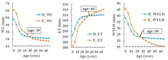
Figure 7.
Changes of hydrological components of different tree species in different forest ages on the hydrologic response unit (HRU) scale. D and E represent deciduous conifers and evergreen conifers, respectively.
Evapotranspiration shows an upward trend with forest aging. During the vegetation growth, the canopy leaves increase, resulting in more trapped water. The transpiration and evaporation of the plant leaves’ trapped water increases, ultimately increasing the amount of evapotranspiration. The growth trend of deciduous conifers’ evapotranspiration was significantly weakened in about 25 years (young forest), and the growth trend of evergreen conifers was similar to that of deciduous conifers. At the age of 40 years (middle-aged forest), the total amount of deciduous conifers’ evapotranspiration exceeded that of deciduous conifers. During the simulation period, the average evapotranspiration of deciduous conifers and evergreen conifers was 306.68 mm and 304.82 mm, respectively, and the evapotranspiration ability of deciduous conifers was slightly stronger.
Total runoff decreases with increased forest aging. The reason for the negative correlation with forest age is the changing forest canopy structure. The increase in leaves reduces the chance of precipitation penetrating through the canopy, and the increased litter also holds some precipitation, thereby reducing water yield ability. The intersection of curves of different tree species’ total runoff appeared at about 30 years. After 30 years, the total runoff of deciduous conifers tended to be stable and began to be greater than that of evergreen conifers. After 30 years, the total runoff of deciduous conifers tended to be stable and began to be greater than that of evergreen conifers. Eventually, the total runoff of evergreen conifers and deciduous conifers was about 15 mm and 21 mm, respectively, and this was still in a downward trend, but the downward trend was deaccelerating.
As a constituent unit of a sub-basin, the changing hydrological components in HRUs affect the hydrological components of the sub-basin. This study changed only some of the attributes of the HRUs in a sub-basin. The variation characteristics of the hydrological components in the sub-basin may differ from those in the HRUs. Studying the hydrological effects of forest age on the sub-basin scale is more similar to the scenario of returning farmland to forest and has more practical significance.
As shown in Figure 8, on the sub-basin scale, the changing trend of hydrological components of different forest types with the aging of trees is similar to that on the HRU scale but shows different characteristics. The intersection of the evapotranspiration curve disappeared, and the evapotranspiration of evergreen conifers on the sub-basin scale was always lower than that of deciduous conifers. There was not much difference in the evapotranspiration of different forest types after reaching maturity, and the difference was less than 1 mm. The patterns of changes in water conservation and total runoff were almost the same as those in HRUs. The patterns of changes in water conservation and total runoff were almost the same as those in HRUs. In the early stage, the two hydrological components of evergreen conifers were greater than those of deciduous conifers. At about 30 years, the relationship between the two began to change, the difference got larger, and the trend of becoming larger tended to be gentle. The long-term water conservation ability of deciduous conifers was slightly stronger.
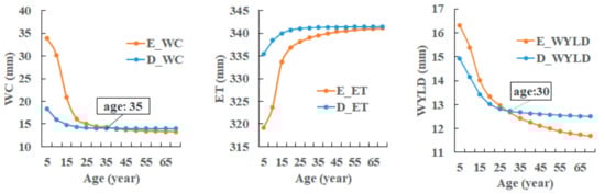
Figure 8.
Changes in hydrological components of different tree species in different forest ages on the sub-basin scale. D and E represent deciduous conifers and evergreen conifers, respectively.
According to People’s Republic of China Forestry Industry Standard and change pattern of curve in Figure 7 and Figure 8, we take trees younger than 40 as a young forest, and those older than 40 as a middle-aged forest and statistically analyze the hydrological effects of forest age and tree species changes on different spatial scale.
Table 7 demonstrates that the change of forest age significantly effects hydrological components on HRU scale, but the difference is slightly weaker on another scale. There are differences among various hydrological components of different tree species, but the differences are not statistically significant. In addition, compared with that on the HRU scale, the difference of hydrological components between different tree species on subbasin scale is more significant.
Table 7.
Analysis of variance of different tree species and different ages on different spatial scale.
5. Discussion
5.1. Discussion
At present, a hydrological model combined with statistical analysis is a common method to clarify the impact of land use changes on hydrological processes. In this study, the SWAT model was used to quantitatively estimate the impact of land use changes on different hydrological components in the Guanting Reservoir basin, and further analyzed the impact of changes in hydrological components on the regional water conservation function. Vegetation can prevent the rapid loss of water after precipitation by canopy interception, litter interception, and by changing the physical structure of the soil and its permeability [43]. Our results show that the declining vegetation coverage reduces evapotranspiration, soil water content, and increases surface runoff and water yield. Water conservation capacity of land uses covered by vegetation is better. This is consistent with previous research results [9]. Among them, forests can effectively reduce runoff and have the strongest water conservation capacity [44,45,46]. However, water conservation characteristics of farmland are different from other vegetation covered systems. Farmland tends to generate more runoff rather than conserve water, the increase in farmland area has a negative effect on regional water conservation, this may be because the use of agricultural machinery further exacerbates the soil compaction [47], and the increase in farmland area increases the surface runoff. Returning farmland to forest can effectively improve the regional water conservation performance [48].
Changes in tree species and forest age will affect the structure of forest, thereby affecting water conservation capacity. Through the method of scenario simulation, in HRU and sub-watersheds, we found that with the forest aging, evapotranspiration increased significantly (p < 0.05) and soil water content and water yield decreased significantly (p < 0.05). The mechanism provided by previous studies [49] shows that as the forest ages, the structure of the forest canopy will change greatly. More and more leaves intercept more precipitation, which makes the evapotranspiration gradually increase, and runoff and water content of the soil decreases. Compared with evergreen conifers, deciduous conifers accumulate more litter on the ground surface. The loose and porous structure results in the stronger water conservation capacity. However, the impact on the hydrological components of tree species change is not statistically significant. Such results are different from previous studies. For example, Gong et al. [38] evaluated the water conservation capacity of different ecosystem types in China, and the results showed that the water conservation capacity of evergreen conifers is higher than that of deciduous conifers. Fan et al. [46] studied the water conservation function of the terrestrial ecosystem at the northern foot of the Qinling Mountains which also showed the same results. It should be noted that most of the research time of the previous researchers was around 2010, which were not long after the implementation of Grain for Green project, and most forests were still young. Therefore, the water conservation capacity of evergreen conifer is stronger than that of deciduous conifer. However, according to the trend of various hydrological components with the aging of the forest, deciduous conifer, which could conserve more water and has similar evapotranspiration capacity to evergreen conifer, has stronger long-term water conservation capacity. Planting deciduous conifers under a rational scheme can improve long-term water conservation capacity.
5.2. Limitations and Future Work
This study has certain limitations in evaluating the impact of changes in land use on regional water conservation. These can be divided into two categories: (1) lack of regional hydrological data, and {2) regional ecological project characteristics. In the process of model calibration, the results show that the measured value of the Guanting station was lower than that of the upstream Xiangshuipu station (Figure 9). As a hydrological station in the Yongding River, under natural conditions, the runoff measured by the Guanting station should be greater than that measured by hydrological stations on the Yanghe River or Sanggan River. The reason for the low measured value of the total outlet is mainly because of the effect of human activities. There is a water transfer project in the study area along with water release from the reservoir, but unfortunately, the water transfer information that could have a great impact on model simulation results has not been collected. Therefore, the area between Shixiali, Xiangshuipu, and Guanting Reservoir was simulated using Xiangshuipu’s calibrated parameters. Figure 9 shows that the simulated value is higher than the measured value at Guanting station. However, the changing trend of the simulated value is consistent with the change of rainfall and is close to the sum of the measured values of Xiangshuipu and Shixiali stations. In the absence of water transfer data, the simulation of natural runoff is still acceptable.
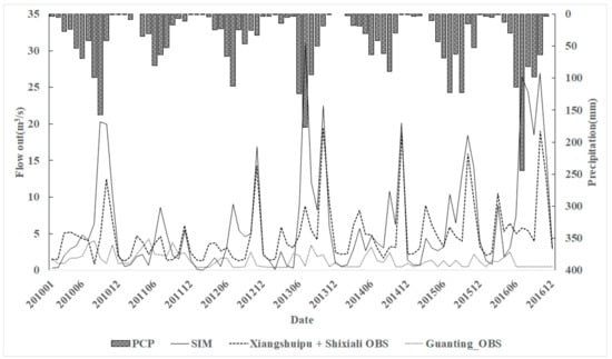
Figure 9.
Comparison between the simulated and observed values of the Guanting Reservoir. PCP denotes precipitation, and OBS and SIM denote observed value and simulated value, respectively.
The specific measures in implementing ecological projects in different regions are different. The afforestation tree species in the study area are mainly coniferous species, e.g., Larix principis and Pinus tabulaeformis. This gives the research on the hydrological effects of forest structure in this study certain limitations. For areas where drastic changes in land use happened, similar land use management methods can be adopted to achieve the sustainable development of water resources. However, for some regions, especially those outside China, the sustainable development of water resources may not necessarily be achieved through large-scale afforestation. Specific land use management methods are still worthy of further discussion. Research on different tree species, especially deciduous trees, will make up deficiencies of this research. When analyzing the influence of forest age on water conservation capacity, to control the terrain and meteorological elements, tree planting operations were added only to certain land uses in a sub-basin. The hydrological effect of forest age under different topographies and meteorological conditions remains to be studied.
6. Conclusions
The hydrological effects of land use changes are significant. In this study, the calibrated and validated SWAT model was used to simulate the changes of different hydrological components in the Zhangjiakou region of the Guanting Reservoir basin in the upper reaches of the Yongding River under the land use scenarios of 2000, 2010, and 2015. The results from the quantitative assessments on historical data indicated that change of land use has a great impact on regional water resources. Most land uses covered by vegetation have strong water conservation capacity. Forests have the strongest water conservation capacity. As the land use turns into forests, the regional water conservation capacity will be improved. Farmland and settlements have poor water conservation capacity, and excessive farmland or settlement area will have a negative impact on the regional water conservation capacity. In forests, water conservation capacity changes significantly with forest age, and there is a negative correlation between them. There are differences in water conservation capacity of different conifer species on different spatial scales, but the difference is not significant. Compared with the HRU scale, the water conservation capacities of different tree species have larger differences on the sub-basin scale. Young evergreen conifers have strong water conservation capacity, but deciduous broad-leaved forests have stronger water conservation capacity in the long term. For the study area, evergreen conifers can be planted to balance the short-term water conservation capacity degradation caused by land use changes, deciduous conifers are more suitable for long-term water conservation function adjustment and planting trees in the study area is an effective method to realize the sustainable development of regional water resources.
Author Contributions
Conceptualization, T.P., L.Z. and F.S.; methodology, T.P.; software, T.P.; validation, Z.Z. (Zijuan Zhu); data curation, Y.L.; writing—original draft preparation, T.P.; writing—review and editing, Z.Z. (Zengxiang Zhang) and X.Z.; visualization, T.P. All authors have read and agreed to the published version of the manuscript.
Funding
This work was funded by A sub-project of China’s National Water Pollution Control and Governance Major Project. Project number 2017ZX07101001005.
Data Availability Statement
The data used to support the findings of this study are available from the corresponding author upon request.
Acknowledgments
Sincerely express our heartfelt thanks to the reviewers and magazine editors for their efforts.
Conflicts of Interest
The authors declare no conflict of interest.
References
- Mittal, N.; Bhave, A.G.; Mishra, A.; Singh, R. Impact of human intervention and climate change on natural flow regime. Water Resour. Manag. 2016, 30, 685–699. [Google Scholar] [CrossRef]
- Palmer, M.A.; Reidy Liermann, C.A.; Nilsson, C.; Flörke, M.; Alcamo, J.; Lake, P.S.; Bond, N. Climate change and the world’s river basins: Anticipating management options. Front. Ecol. Environ. 2008, 6, 81–89. [Google Scholar] [CrossRef]
- Rose, S.; Peters, N.E. Effects of urbanization on streamflow in the Atlanta area (Georgia, USA): A comparative hydrological approach. Hydrol. Process. 2001, 15, 1441–1457. [Google Scholar] [CrossRef]
- Wang, R.; Kalin, L. Combined and synergistic effects of climate change and urbanization on water quality in the Wolf Bay watershed, southern Alabama. J. Environ. Sci. 2018, 64, 107–121. [Google Scholar] [CrossRef] [PubMed]
- Wang, M.; Du, L.; Ke, Y.; Huang, M.; Zhang, J.; Zhao, Y.; Li, X.; Gong, H. Impact of climate variabilities and human activities on surface water extents in reservoirs of Yongding River basin, China, from 1985 to 2016 based on Landsat observations and time series analysis. Remote Sens. 2019, 11, 560. [Google Scholar] [CrossRef]
- Woldesenbet, T.A.; Elagib, N.A.; Ribbe, L.; Heinrich, J. Hydrological responses to land use/cover changes in the source region of the Upper Blue Nile basin, Ethiopia. Sci. Total Environ. 2017, 575, 724–741. [Google Scholar] [CrossRef]
- Meng, F.; Liu, T.; Wang, H.; Luo, M.; Duan, Y.; Bao, A. An alternative approach to overcome the limitation of HRUs in analyzing hydrological processes based on land use/cover change. Water 2018, 10, 434. [Google Scholar] [CrossRef]
- Dias, L.C.P.; Macedo, M.N.; Costa, M.H.; Coe, M.T.; Neill, C. Effects of land cover change on evapotranspiration and streamflow of small catchments in the Upper Xingu River basin, Central Brazil. J. Hydrol. Reg. Stud. 2015, 4, 108–122. [Google Scholar] [CrossRef]
- Wang, G.; Yang, H.; Wang, L.; Xu, Z.; Xue, B. Using the SWAT model to assess impacts of land use changes on runoff generation in headwaters. Hydrol. Process. 2014, 28, 1032–1042. [Google Scholar] [CrossRef]
- Li, Q.; Zhang, J. Rejuvenating coal energy industry of Shanxi Province through devoting major efforts to developing briquette industry. Sci./Tech Inf. Dev. Econ. 2000, 10, 17–19. [Google Scholar] [CrossRef]
- Wang, H.; Zheng, S. Opinions about development of iron and steel industry of Hebei Province. Hebei Metallurgy. Hebei Metall. 2005, 3–6. [Google Scholar] [CrossRef]
- Gu, S.; Lu, C.; Qiu, J. Quantifying the degree of water resource utilization polarization: A case Study of the Yellow River basin. J. Resour. Ecol. 2019, 10, 21. [Google Scholar] [CrossRef]
- Wang, L.; Wang, Z.; Koike, T.; Yin, H.; Yang, D.; He, S. The assessment of surface water resources for the semi-arid yongding river basin from 1956 to 2000 and the impact of land use change. Hydrol. Process. 2010, 24, 1123–1132. [Google Scholar] [CrossRef]
- Ma, Z.; Li, L.; Yang, R.; Wang, B. Assessment and countermeasures of ecosystem health in the Beijing-Zhangjiakou Area. Arid Zo. Res. 2019, 36, 228–236. [Google Scholar] [CrossRef]
- Dwarakish, G.; Ganasri, B. Impact of land use change on hydrological systems: A review of current modeling approaches. Cogent Geosci. 2015, 1, 1–18. [Google Scholar] [CrossRef]
- Che, Q.; Wang, G.; Kong, F.; Chen, L.; Jiang, X. Runoff estimation under climate and land cover change in yellow river source region. J. China Hydrol. 2007, 27, 11–15. [Google Scholar] [CrossRef]
- Guo, H.; Hu, Q.; Jiang, T. Annual and seasonal streamflow responses to climate and land-cover changes in the Poyang Lake basin, China. J. Hydrol. 2008, 355, 106–122. [Google Scholar] [CrossRef]
- Li, B.; Shi, X.; Lian, L.; Chen, Y.; Chen, Z.; Sun, X. Quantifying the effects of climate variability, direct and indirect land use change, and human activities on runoff. J. Hydrol. 2020, 584, 1–11. [Google Scholar] [CrossRef]
- Zhang, H.; Wang, B.; Liu, D.L.; Zhang, M.; Leslie, L.M.; Yu, Q. Using an improved SWAT model to simulate hydrological responses to land use change: A case study of a catchment in tropical Australia. J. Hydrol. 2020, 585, 1–15. [Google Scholar] [CrossRef]
- Bormann, H.; Breuer, L.; Gräff, T.; Huisman, J.A. Analysing the effects of soil properties changes associated with land use changes on the simulated water balance: A comparison of three hydrological catchment models for scenario analysis. Ecol. Modell. 2007, 209, 29–40. [Google Scholar] [CrossRef]
- Song, Y.; Ma, J. SWAT-aided research on hydrological responses to ecological restoration: A case study of the Nanhe River basin in Huajialing of Longxi Loess Plateau. Acta Ecol. Sin. 2008, 28, 636–644. [Google Scholar] [CrossRef]
- Chen, L.; Chen, S.; Li, S.; Shen, Z. Temporal and spatial scaling effects of parameter sensitivity in relation to non-point source pollution simulation. J. Hydrol. 2019, 571, 36–49. [Google Scholar] [CrossRef]
- Cui, G.; Wang, X.; Li, C.; Li, Y.; Yan, S.; Yang, Z. Water use efficiency and TN/TP concentrations as indicators for watershed land-use management: A case study in Miyun District, north China. Ecol. Indic. 2018, 92, 239–253. [Google Scholar] [CrossRef]
- Ke, Q.; Zhao, J.; Wang, S.; Zheng, W.; Yin, D. Application of total maximum daily load(TMDL) in control of agricultural non-point source pollution and its developmental trend. J. Ecol. Rural Environ. 2009, 25, 85–91. [Google Scholar] [CrossRef]
- Lin, G.; Zeng, H.; Xie, J. Application of SWAT model in basin LUCC hydrological effect. J. Water Resour. Water Eng. 2009, 20, 145–151. [Google Scholar]
- Fornell, C.A. Second Generation of Multivariate Analysis: An Overview, 1st ed.; Praeger: San Francisco, CA, USA, 1982. [Google Scholar]
- Wold, S.; Albano, C.; Dun, M. Pattern regression finding and using regularities in multivariate Data. In Proceedings of the Pattern Regression Finding and Using Regularities in Multivariate Data; Analysis Applied Science Publication: London, UK, 1983; pp. 147–188. [Google Scholar]
- Chen, J.; Li, X. Simulation of hydrological response to land-cover changes. Chin. J. Appl. Ecol. 2004, 15, 833–836. [Google Scholar]
- Wang, H.; Sun, F.; Xia, J.; Liu, W. Impact of LUCC on streamflow based on the SWAT model over the Wei River basin on the Loess Plateau in China. Hydrol. Earth Syst. Sci. 2020, 21, 1929–1945. [Google Scholar] [CrossRef]
- Wang, X.; Zhang, P.; Liu, L.; Li, D.; Wang, Y. Effects of human activities on hydrological components in the Yiluo River basin in Middle Yellow River. Water 2019, 11, 689. [Google Scholar] [CrossRef]
- Sun, X.; Wang, G. A review of forest hydrology study and its spatial pattern for dark coniferous forest in Gongga Mountain, Southwest China. Mt. Res. 2017, 35, 677–685. [Google Scholar] [CrossRef]
- Wilson, K.B.; Hanson, P.J.; Mulholland, P.J.; Baldocchi, D.D.; Wullschleger, S.D. A comparison of methods for determining forest evapotranspiration and its components: Sap-flow, soil water budget, eddy covariance and catchment water balance. Agric. For. Meteorol. 2008, 106, 153–168. [Google Scholar] [CrossRef]
- Savenije, H.H.G. The importance of interception and why we should delete the term evapotranspiration from our vocabulary. Hydrol. Process. 2004, 18, 1507–1511. [Google Scholar] [CrossRef]
- Li, H. Impact analysis of historical forest change on Yongding River. China Water Resour. 2005, 18, 23. [Google Scholar]
- O’connell, P.E.; Nash, J.E.; Farrell, J.P. River flow forecasting through conceptual models patr II-the brosna catchment at ferbane. J. Hydrol. 1970, 10, 282–290. [Google Scholar] [CrossRef]
- Liew, M.W.; Garbrecht, J. Hydrologic simulation of the Little Washita River experimental watershed using SWAT. J. Am. Water Resour. Assoc. 2003, 39, 413–426. [Google Scholar] [CrossRef]
- Morias, D.; Arnold, J.; Van Liew, M.W.; Bingner, R.; Harmel, R.D.; Veith, T.L. Model evaluation guidelines for systematic quantification of accuracy in watershed simulations. Trans. ASABE 2007, 50, 885–900. [Google Scholar] [CrossRef]
- Gong, S.; Xiao, Y.; Zheng, H.; Xian, Y.; Ouyang, Z. Spatial patterns of ecosystem water conservation in China and its impact factors analysis. Acta Ecol. Sin. 2017, 37, 2455–2462. [Google Scholar] [CrossRef]
- Wang, C.; Li, G.; Bai, W.; Wang, H.; Shi, J.; Gao, C.; Wen, G. People’s Republic of China Forestry Industry Standard; National Forestry Administration: Beijing, China, 2018; pp. 5–9. [Google Scholar]
- Zhou, G.; Yin, G.; Tang, X.; Wen, D.; Liu, C.; Kuang, Y.; Wang, W. China’s Forest Ecosystem Carbon Storage: Biomass Equation, 1st ed.; Science Press: Beijing, China, 2018. [Google Scholar]
- Jiang, Y.; Deng, H.; Gao, D.; Xia, C. Constructing height-diameter curve equations with measurement error models for Chinese pine stands. J. Northeast For. Univ. 2015, 43, 126–129. [Google Scholar] [CrossRef]
- Chai, Z. The Study on Growth Characteristics and Close-Nature Management Techniques for Larix-principis-rupprechtii Artificial Forest; Northwest A&F University: Xianyang, China, 2013. [Google Scholar]
- Cui, L. Evaluation on functions of Poyang Lake ecosystem. Chin. J. Ecol. 2004, 23, 47–51. [Google Scholar]
- Dai, J.; Chen, J.; Cui, Y.; He, Y.; Ma, J. Impact of forest and grass ecosystems on the water budget of the catchments. Adv. Water Sci. 2005, 17, 435–443. [Google Scholar] [CrossRef]
- Sriwongsitanon, N.; Taesombat, W. Effect of land cover on runoff coefficient. J. Hydrol. 2011, 410, 226–238. [Google Scholar] [CrossRef]
- Fan, Y.; Liu, K.; Chen, S.; Yuan, J. Spatial pattern analysis on water conservative functionality of land ecosystem in northern slope of qinling mountains. Bull. Soil Water Conserv. 2017, 37, 50–56. [Google Scholar] [CrossRef]
- Shi, Y.; Chen, Y.; Sui, P.; Nie, Z.; Gao, W. Cropland soil compaction: Its causes, influences, and improvement. Chin. J. Ecol. 2010, 29, 2057–2064. [Google Scholar] [CrossRef]
- Liang, W.; Bai, C.; Sun, B.; Qu, J. Soil water availability and soil water storage capacity in forest or grass Lands converted from farmlands in Loess Hilly and Gully Region—A case study of Chaigou watershed in Wuqi County. Bull. Soil Water Conserv. 2006, 26, 38–40. [Google Scholar] [CrossRef]
- Ma, X. Forest Hydrology; China Forestry Publishing House: Beijing, China, 1993. [Google Scholar]
Publisher’s Note: MDPI stays neutral with regard to jurisdictional claims in published maps and institutional affiliations. |
© 2020 by the authors. Licensee MDPI, Basel, Switzerland. This article is an open access article distributed under the terms and conditions of the Creative Commons Attribution (CC BY) license (http://creativecommons.org/licenses/by/4.0/).