Article

Competitive Pricing of Innovative Products with Consumers’ Social Learning

1
School of Management, Guangdong University of Technology, Guangzhou 510520, China
2
China Development Bank Hubei Branch, Wuhan 430061, China
3
Training Base, Army Logistics University of PLA, Wuhan 430035, China
*
Authors to whom correspondence should be addressed.
Sustainability 2020, 12(9), 3806; https://doi.org/10.3390/su12093806
Submission received: 27 March 2020 / Revised: 4 May 2020 / Accepted: 6 May 2020 / Published: 7 May 2020
(This article belongs to the Section Economic and Business Aspects of Sustainability)

Abstract

:
Consumers often face valuation uncertainty when innovative products are introduced into market, and they may update the valuation about product quality based on historical sales information over time. Based on this background, this study constructed a two-period duopoly model of innovative products and investigated the effect of consumers’ social learning on enterprises’ pricing strategies and profits. Optimal pricing decisions for competitive enterprises with and without consumers’ social learning were obtained. It was found that consumers’ social learning will intensify competition between enterprises, which will lower their prices and profits. The stronger the learning intensity of consumers, the greater the profit loss for enterprises.

1. Introduction

In many innovative product and experience good markets, the consumer does not recognize the precise value of the product before consumption. For example, when a new hybrid car is launched, a consumer might not be able to predict its fuel efficiency and battery life. When a new software is released, a consumer might not be able to precisely anticipate its performance and stability. This scenario is also prevalent in other newly innovated electronic products, such as smart phones and tablet computers, and other industries, such as apparel industries [1].
Consumers can acquire more information about an innovative product from several sources and evaluate the product better over time [2], such as peer consumer reviews and historical sales on e-commerce websites. The influence of consumer reviews and historical sales on the purchase decisions of potential product buyers has grown dramatically in the last decade, with recent surveys suggesting that up to 69% of consumers will consult peer reviews before determining whether to buy a product [3]. To date, efforts in this area of research have focused on a monopoly’s pricing strategy of experience good, or duopoly competition with a consumer learning mechanism driven by Bayesian inference. To fill the gap, this paper tries to research the competitive pricing strategies of innovative products considering a non-Bayesian learning mechanism.
This study aimed to investigate the effect of consumers’ social learning on duopoly enterprises. Based on the Hotelling competition model, this study constructed a two-period competition model considering consumers’ social learning. The main research questions are as follows:
  • Considering consumers’ social learning, how will competitive enterprises set product prices?
  • How will the demand and profits of competitive enterprises change with consumers’ social learning?
  • How will learning intensity and product quality affect enterprises’ profits under consumers’ social learning?
Next, Section 2 presents the literature review, which introduces the state of research on pricing of innovative products and social learning theory. Section 3 presents a two-period competition model that does not consider consumers’ social learning, which we call the benchmark model. In Section 4, a two-period competition model that considers consumers’ social learning is constructed to obtain the optimal pricing strategies for enterprises and changes in demand. This model is then compared to the benchmark model to study the effect of consumers’ social learning on enterprises’ prices and profits. Section 5 explores the effect of learning intensity and product-quality gap on enterprises’ profits. Finally, Section 6 summarizes the study and makes suggestions for future research.

2. Literature Review

This paper is related to two streams of the literature: social learning, and pricing of innovative products and experience goods.
Social learning in economics originated from the paper by Banerjee [4], which found that observing decision-making by others leads to herd behavior under certain assumptions—that is, people imitate others’ behaviors regardless of the information they own. To study economic phenomena under long-term learning, Banerjee and Fudenberg [5] constructed a model to convey information through language, which relaxed the assumption of the exogenous decision-making order of individuals so that individuals could use information from previous individuals to judge benefits themselves.
Since individual learning is often related to acquired signals, some studies have examined the signal problem in social learning. Dividing the signals individuals obtain into two-point signals and Gaussian signals, Chamley [6] analyzed how individual beliefs are updated under the two signal types, compared the convergence rate of the two kinds of learning signals, and applied these two updating processes to an economic model. Two-point signals and Gaussian signals are widely used because of their good analytical properties. Gallego, et al. [7] studied the design problem of product-delay service. In that study, consumers updated their judgments about the probability of product damage over time; beta updates and exponential stationary updates were introduced, and the signals in these two types of updates were both two-point signals. Kwon, et al. [8] studied the investment problem of uncertain income when Bayesian learning and externality exist. That study assumed that investors who enter the market later can observe the returns of investors who enter the market first, and thus judge the state of the market. The return for investors who enter the market first is observed as a signal by investors who enter later, and this signal is a Gaussian signal. According to the degree of signal acquisition, the signal is divided into fully observed and partially observed signals. In the social learning literature based on Banerjee, it is always assumed that all signals are observable; in reality, however, the signals observed by individuals may be limited. Celen, et al. [9] studied the change in Bayesian learning in the network when individuals could only observe the behavior of their neighbors. Acemoglu, et al. [10] studied models of individuals observing the behavior of some pioneers through a random process. They found that progressive learning will happen when the social network is large enough and the signal is fully observable; it might also occur when the signal is only partially observable. Callander and Hoerner [11]’s hypothesis on signal observation differed from Acemoglu’s. They assumed that individuals can choose the signals they want to observe instead of going through a random process. According to the difficulty of signal acquisition, a social learning model with observation cost appears. Song [12] extended the process of the individual observation of information to an endogenous situation—that is, the individual observation of signals requires a cost, and individuals can choose whether to pay the cost to obtain signals. That study found that learning with a cost will obtain better learning results than learning without a cost.
Social learning models have been widely studied in operation management markets that focus on enterprises and consumer decisions. As the main body of the market, consumers and enterprises often update their judgments about the state of the market according to information in the market, thus changing their pricing and purchasing decisions. Yu, et al. [13] constructed a two-stage dynamic pricing model and studied the influence of consumers’ collective comments on enterprises’ pricing decisions. In that study, the models in operation management were classified into unilateral and bilateral learning models according to the learning subject. As its name implies, in a unilateral learning model, only one end of the market can obtain information. Enterprises can estimate market size more accurately through learning. Petruzzi and Dada [14] also found that enterprises use the demand of one stage to estimate the demand of the next stage and derive optimal inventory decisions. Consumers can update their judgments about product value through learning. Subramanian and Rao [15] suggested that the number of consumers who have purchased products will attract new consumers. Enterprises can publish the number of consumers who have purchased products through a third-party platform, and the third-party platform decides whether to publish the information. Learning behavior gives consumers an opportunity to understand the true quality of a product, thus promoting the emergence of strategic customers. Ovchinnikov and Milner [16] studied strategic consumers’ learning about corporate discount strategies. Allon and Bassamboo [17] studied enterprises’ choices about whether to strategically disclose information to consumers. Through this method, enterprises can influence consumers’ perceptions to influence their willingness to pay and control market demand. Papanastasiou and Savva [18] used a two-period model to study how social learning affects the strategic interaction between a dynamic-pricing monopolist and a forward-looking consumer population.
This paper is also related to several models of dynamic pricing of experience goods. Villas-Boas [19] considered price competition in a two-period model to study the effect of potential informational advantage of experience goods, and found that the skewness of consumer value distribution is the primary factor driving brand loyalty and firm profits. Villas-Boas [20] extended the above dynamic competition model of experience goods to an infinite horizon with overlapping generations of consumers, and found that the higher the prices and profits, the greater the probability of perfect product fit. Bergemann and Valimaki [21] showed that the monopoly price of an experience good declines over time in a mass market but may increase in a niche market. However, they examine self-learning about experience goods through repeat purchase, whereas we consider social learning about an experience good. Several papers have also examined pricing strategies of experience goods with social learning. Feldman, Papanastasiou and Segev [3] studied the interaction between review-based social learning and a monopolist firm’s choice of product price and design. Differently from this study, our study concentrated on competitive pricing strategies of innovative goods with social learning. The closest literature to our paper is Jing [22], who studied the effects of behavior-based price discrimination in a two-period experience good duopoly and examined the role of consumers’ ex ante valuation uncertainty in dynamic price competition through comparison with an inspection good duopoly. That paper considered a consumer learning mechanism driven by Bayesian inference, but our paper considered a non-Bayesian learning mechanism.

3. Model without Consumer Learning

In this section, we present a two-period model for duopoly enterprises that does not consider consumers’ social learning; we call this the benchmark model. We first provide the basic assumptions of the model and then analyze its equilibrium results.

3.1. Basic Assumptions

We consider a two-period model of innovative products competition. Suppose there is a duopoly market that sells innovative products. The two enterprises are located at both ends of a linear city unit and are denoted as enterprise 0 and enterprise 1. They sell innovative products in two periods. Product 0 is initiated by enterprise 0, and product 1 is initiated by enterprise 1. The total amount of consumers is normalized to 1 and is uniformly distributed in the linear city. In each period, consumers arrive at the market, and each consumer can purchase, at most, one product. Each consumer knows his or her distance from the seller. Assume a per-unit cost of “traveling” to the product being purchased is φ . The transportation cost can be seen as the cost to arrive at the firm, such as transport expense or a network fee. When a consumer buys products at distance   x , he or she needs to pay transportation cost φ x . In the analysis later in this paper, we normalize the unit transportation cost   φ   to 1.
Competition between enterprises is reflected in the choices of consumers, who choose from two kinds of innovative products in each period. Naturally, consumers will compare the quality of the two products. Assume the probability that consumers think product 0 is of higher quality than product 1 is   α , and the probability that product 1 is of higher quality than product 0 is   1 α . Consumers’ valuation of low-quality products is v 0 , and that of high-quality products is v 0 + m , where m represents the valuation gap between high-quality and low-quality products. Assume v 0   is high enough to cover the whole market.
Since the quality of innovative products is often difficult to estimate, it is also difficult for consumers to compare the quality of two products. In such an uncertain situation, consumers’ estimations of product quality will change with time. Let v i t   denote consumers’ quality estimation of product   i at period   t , where   i = { 0 ,   1 }, t = { 1 ,   2 } . Before the selling season, enterprise 0 and enterprise 1 set the product price as p 0   and   p 1 , and the prices stay unchanged in both periods. For a consumer located at   x in the linear city, the utility of buying product 0 and product 1 at period   t is   u 0 t = v 0 t x p 0 and u 1 t = v 1 t ( 1 x ) p 1 , respectively. Consumers will choose to buy products with higher utility. There is competition between the two enterprises, and the product price they set will affect the product demand of both sides. Enterprises obtain the equilibrium price by maximizing the sum of profits in the two periods. The cost of the product is normalized to 0. Assume that consumers and enterprises are risk-neutral, and the influence of time discounting is not considered in the model.

3.2. Benchmark Model

When not considering consumers’ social learning, consumers do not update their estimation of product quality based on historical product sales, and the probability that consumers think that product 0 is of higher quality than product 1 is always   α . In this situation, the enterprise’s demand in the first and second period will not change. The utility of consumers located at x from buying product 0 and product 1 is
u 0 = v 0 + α m x p 0 ,
u 1 = v 0 + ( 1 α ) m ( 1 x ) p 1 .
Theorem 1.
Without consumers’ social learning, a unique pure strategic equilibrium exists when m < 3 . In this equilibrium, p 0 * = 1 + ( 2 α 1 ) m 3 , p 1 * = 1 + ( 1 2 α ) m 3 ; and the corresponding optimal profit is   π 0 * = [ 3 + ( 2 α 1 ) m ] 2 9 , π 1 * = [ 3 + ( 1 2 α ) m ] 2 9 .
Proof is shown in Appendix A. Without consumers’ social learning, an enterprise’s advantage in the market depends on the probability α that consumers think product 0 is of higher quality than product 1. From Theorem 1, we can intuitively derive the following conclusions. First, when α > 1 2 , consumers prefer the products of enterprise 0, which will attain market advantage and obtain more benefits. Second, when α > 1 2 , the price set by firm 0 will be higher than the price set by firm 1. Third, when α > 1 2 , the profit of the dominant firm monotonously increases with m . In the benchmark model, the sales of period one and period two are exactly the same and do not vary.

4. Model with Consumer Learning

In this section, we present a two-period competition model that considers consumers’ social learning. First, the process of consumers’ social learning is described. Then, the decision-making process is given, and the equilibrium results of the model are analyzed. Finally, the effect of consumers’ social learning on duopoly enterprises’ pricing and profits is studied through comparison with the benchmark model.

4.1. Process of Consumers’ Social Learning

Consumers’ social learning process is reflected in the variation in their estimations of product quality. Consumers arriving in the second phase can observe the sales situations of product 0 and product 1 in the first phase and update their judgments about product quality accordingly. For consumers arriving in the first period, the probability that they think product 0 is of higher quality than product 1 is α ; their expected quality estimation of product 0 is   v 0 1 = v 0 + α m , and that of product 1 is v 1 1 = v 0 + ( 1 α ) m . Suppose the sales quantity of product 0 in the first period is x 1 , and the sales quantity of product 1 in the first period is   1 x 1 .
Consumers arriving in the second period can observe the purchase history of the first period and update their estimation of product quality. Consumers believe product sales represent product quality information—the higher the sales, the better the quality. If the sales quantity of product 0 in the first period x 1 is higher than probability   α , consumers will think the quality of the product is better than imagined and update the probability to α > α . Accordingly, if x 1 is lower than α , they will think the quality of the product is worse than imagined and update the probability to α < α . In the second period, consumers update the probability that product 0 is of higher quality than product 1 to α = α + β ( x 1 α ) ; accordingly, consumers update the probability that product 1 is of higher quality than product 0 to   1 α = 1 α + β [ ( 1 x 1 ) ( 1 α ) ] . Such product-quality updating behavior is actually a process of consumers’ social learning. β ( 0 < β < 1 ) measures the products’ inherent social strength and is called its consumer learning intensity. This reflects the propensity that its attribute information disseminates among peer consumers via social forces and represents the impact degree of the consumer’s learning behavior. More specifically, it is the tendency of the product’s attributes and functions to be discussed through online or offline word of mouth. A higher β indicates stronger consumer learning and a product with more chat-worthy features. Our notion of social learning intensity corresponds to the intensity of word-of-mouth recommendation in Jing [23]. Under this learning behavior by consumers, their two-period utility function can be expressed as
u 0 1 = v 0 + α m x p 0 ,
u 1 1 = v 0 + ( 1 α ) m ( 1 x ) p 1 ,
u 0 2 = v 0 + α m x p 0 ,
u 1 2 = v 0 + ( 1 α ) m ( 1 x ) p 1 .

4.2. Decision-Making Process

When considering consumers’ social learning, the decision-making process of the model is as follows. Before period 1, firm 0 and firm 1 declare the products’ prices, p 0 and p 1 , at the same time. In period 1, the arriving consumers choose to buy a product between firm 0 and firm 1 according to their expected utility. At the end of period 1, product demand is realized, where the demand for product 0 is   x 1 , and the demand for product 1 is   1 x 1 . In period 2, arriving consumers can observe the demand for products in period 1, update their own estimations of product quality, and choose between product 0 and product 1 according to the updated utility. At the end of period 2, product demand is realized, where the demand for product 0 is   x 2 , and the demand for product 1 is   1 x 2 .
Figure 1 shows the decision-making process of the model. Under this process, we explore the pure strategic equilibrium of the model.

4.3. Equilibrium Analysis

When considering consumers’ social learning, firm 0 and firm 1 determine optimal product prices p 0 and p 1 to maximize their total profits from the two periods. Considering time value, the profits of period 2 should be discounted at discount factor δ . For simplicity, we assume a discount factor of   δ = 1 and neglect its influence in our analysis. The total demand for product 0 is   x 1 + x 2 ; the total demand for product 1 is 2 x 1 x 2 . Therefore, the profits of firm 0 and firm 1 are   π 0 = ( x 1 + x 2 ) p 0 and π 1 = ( 2 x 1 x 2 ) p 1 .
Theorem 2.
With consumers’ social learning, a unique pure strategic equilibrium exists when   6 ( 2 + β m β ) m > 0 . In this equilibrium, p 0 * = 6 + ( 2 α 1 ) ( 2 + β m β ) m 3 ( 2 + β m ) , p 1 * = 6 + ( 1 2 α ) ( 2 + β m β ) m 3 ( 2 + β m ) , and the corresponding optimal profit is   π 0 * = [ 6 + ( 2 α 1 ) ( 2 + β m β ) m ] 2 18 ( 2 + β m ) , π 1 * = [ 6 + ( 1 2 α ) ( 2 + β m β ) m ] 2 18 ( 2 + β m ) .
Proof is shown in Appendix A. From Theorem 2, we can observe an equilibrium result similar to Theorem 1. With consumers’ social learning, when α > 1 2 , consumers prefer the products of enterprise 0, which will attain market advantage and obtain more benefits by setting a higher price. Meanwhile, the profits of the two enterprises decrease with consumers’ learning intensity, β . For enterprises, the higher the consumer’s estimation of product quality, the stronger the attraction of their products. Enterprises can use this advantage to set higher prices to achieve higher profits. This advantage also increases with the increase in the valuation gap between the products. Meanwhile, consumers’ social learning behavior also has an internal effect on enterprises’ decision-making processes. For enterprises, the prices they set not only directly affect the demand of the two periods but also indirectly affect consumers’ updating of product quality. Through pricing, an enterprise can control the demand of period 1, thus controlling consumers’ estimations of product quality in period 2, and the variation in quality estimation will affect the demand of period 2.
Theorem 3.
When α < 1 2 , firm 0′s demand in period 2 will expand, namely, x 2 > x 1 . When α = 1 2 , the two firms’ demand will remain unchanged. When α > 1 2 , firm 0′s demand in period 2 will decrease, namely, x 2 < x 1 .
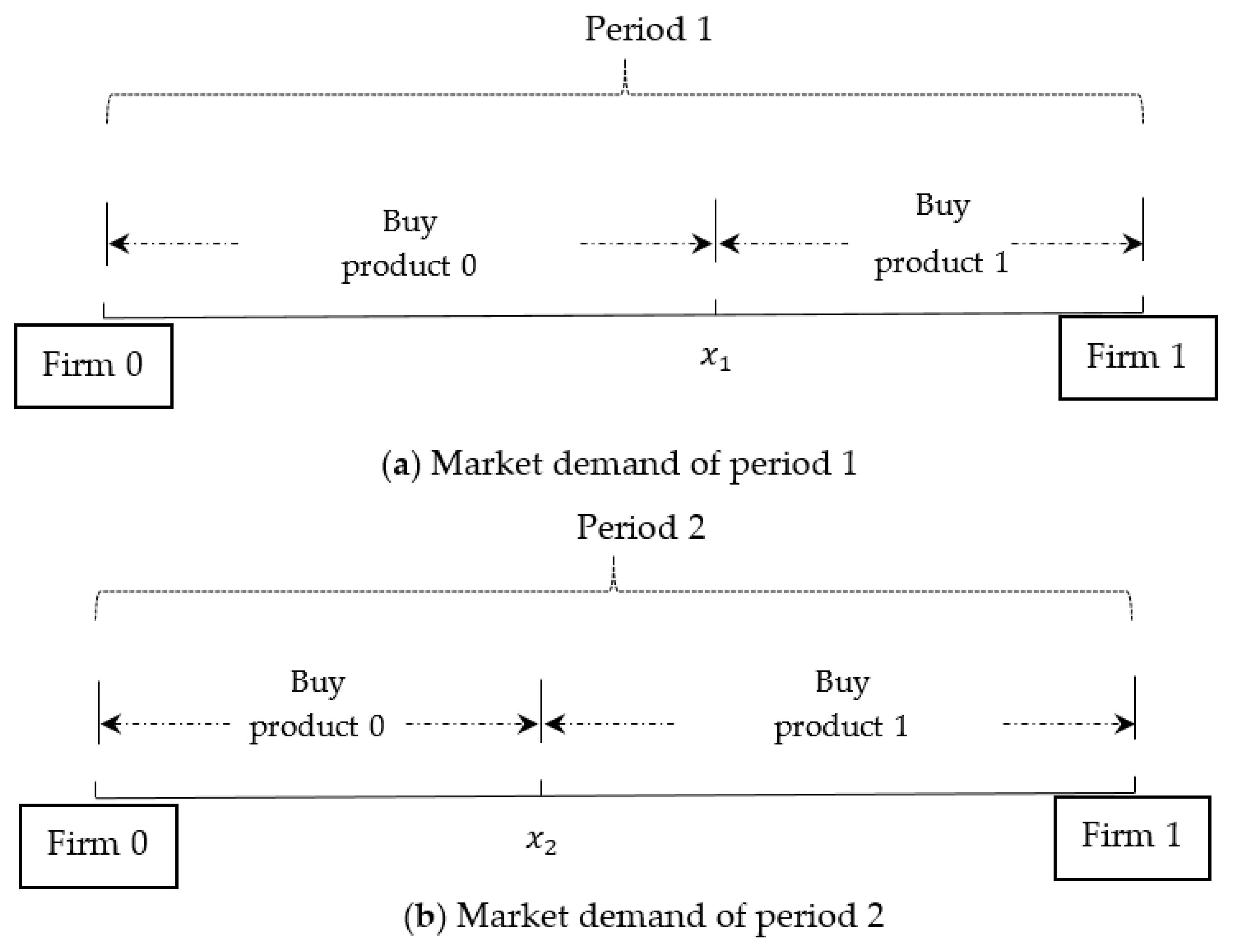
Proof is shown in Appendix A. We know from Theorem 3 that when α > 1 2 , i.e., consumers think product 0 is of higher quality than product 1, firm 0 occupies a dominant market share in period 1. The equilibrium price of product 0 is higher than that of product 1. As a result, the equilibrium demand of product 0 in period 1 ( x 1 ) is less than α . Due to consumers’ social learning, the price increment set by the firm 0 is not enough to make the sales volume of product 0 in period 1 high enough for consumers to observe. Thus, consumer quality estimation in period 2 decreases, and the demand for product 0 in period 2 also decreases. When α = 1 2 , consumers believe the two products are exactly the same, the sales volume of each period is 1 2 , and consumers will not change their judgment about product quality. When α < 1 2 , although the sales of firm 0 in the first period is rather low, the proportion of its sales is higher than α . Sales in the first period increase consumers’ estimations of product quality in the second stage, eventually making the sales of period 2 increase. Consumers’ social learning behavior is the main reason for the variation in product sales volume in the two periods. Variations in consumers’ estimations of product quality make it more difficult for enterprises to predict market demand and set accurate prices.
Figure 2 shows the market demand in the two periods when   α > 1 2 .
Theorem 4.
Compared to the benchmark model, when considering consumers’ learning behavior, p i * < p i * , i = { 0 ,   1 } .
Proof is shown in Appendix A. Theorem 4 shows that consumers’ social learning intensifies the competition between enterprises. To ensure more demand in the first period, enterprises have to lower their prices. Consumers’ learning behavior causes enterprises to pay more attention to the sales situation of products in period 1. Enterprises must strengthen the competition between themselves to occupy a higher market share at a lower price. On the contrary, consumers’ social learning increases their utility, which benefits from the lower prices set by enterprises. When   α = 1 2 , consumer valuation of the product does not change, but enterprises predict that social learning will occur among consumers. Therefore, enterprises will pay more attention to the sales in period 1 and still lower the price. Furthermore, this price reduction has a greater effect on advantage enterprises. When α > 1 2 , firm 0 has advantage in the market, and its price reduction is greater than that of firm 1 compared to the benchmark model. Moreover, the reduction in enterprise pricing is also related to consumers’ learning intensity; the stronger the learning intensity, the greater the effect of consumers’ social learning behavior on the market, and the greater the degree of change in enterprise pricing.
Theorem 5.
Compared to the benchmark model, when considering consumers’ learning behavior, π i * < π i * ,   i { 0 ,   1 } .
Proof is shown in Appendix A. While Theorem 4 explains enterprises’ price changes, Theorem 5 is more concerned with the change in enterprises’ profits. Theorem 5 shows that consumers’ social learning will not only cause prices to fall but also lowers enterprises’ profits. Consumers’ updating of product valuation is a kind of psychological behavior. No matter how consumers update, the products they finally obtain will remain unchanged. When there is competition in the market, and the market is completely occupied by enterprises, the social learning phenomenon of consumers reduces enterprises’ profits. This is because, in the two-stage market, the total size of the market is two and will not change with consumer learning. Therefore, under limited market scale competition, enterprises must reduce prices to gain a higher market share in the first period, which also leads to a decline in enterprises’ profits. Meanwhile, the consumer surplus will increase under consumers’ social learning, which also shows that consumers’ social learning is beneficial to consumers in the case of competition. For enterprises, in the case of competition, they are more willing to hide sales volumes in the market.

5. Static Comparative Analysis

With consumers’ social learning, enterprises’ profits will be reduced. The extent of the reduction is closely related to the valuation gap m of high-quality and low-quality products and the intensity of consumer learning   β . In this section, we will explore the effect of m and β   on enterprise’s revenue losses.

5.1. Effect of Quality Gaps

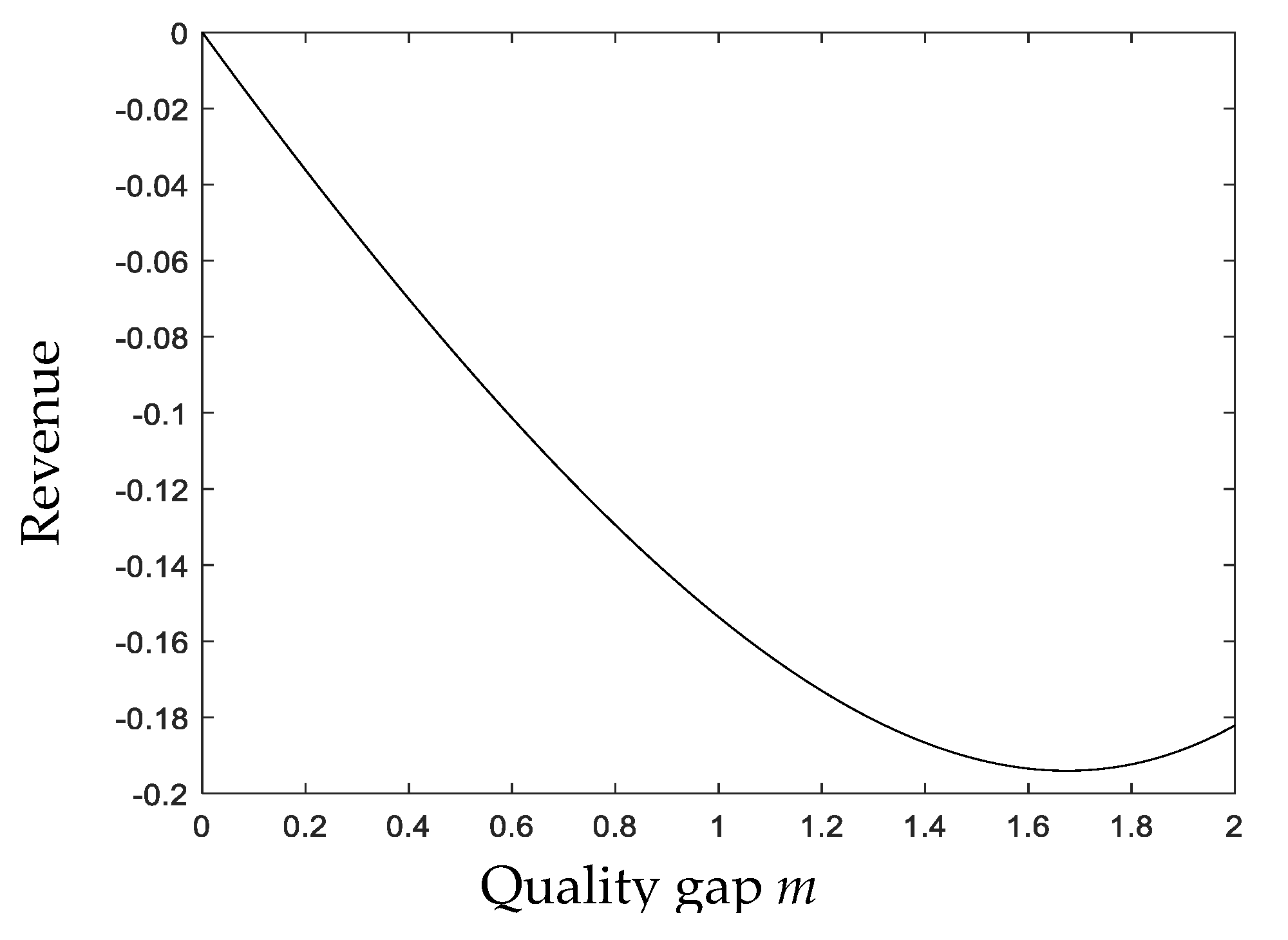
In the above two models, when the probability α that consumers think that product 0 is of higher quality than product 1 is greater than 1 2 , enterprise 0′s revenue increases with valuation gap m of high-quality and low-quality products. This is intuitive to understand. Higher m represents higher valuation of product 0, thus enterprise 0 can set a higher price and gain higher revenue. However, the variation ranges of enterprise revenue with respect to m in the two models are not the same.
Figure 3 describes how enterprise 0′s revenue loss varies with respect to quality gap m , when α = 0.1 , β = 0.8 ; where the probability α that consumers think product 0 of higher quality than product 1 is smaller than 1 2 , enterprise 0 is at a disadvantaged position. Let the valuation gap m of high-quality and low-quality products vary from 0 to 2. In this case, the parameters satisfy the prerequisite of the existence of equilibrium in the two models. As seen from Figure 3, enterprise 0′s profit loss is non-monotonic with respect to m . When m is small, the equilibrium price of product 0 and the equilibrium profit of enterprise 0 decreases with the increment of m . Then, consumers’ learning behavior makes inferior enterprise’s revenue loss increase with   m . When m increases to a certain extent, the equilibrium demand of product 0 is too small for consumers to observe. Therefore, inferior enterprise’s revenue loss shows a trend of small reduction with   m .

5.2. Effect of Intensity of Consumer Learning

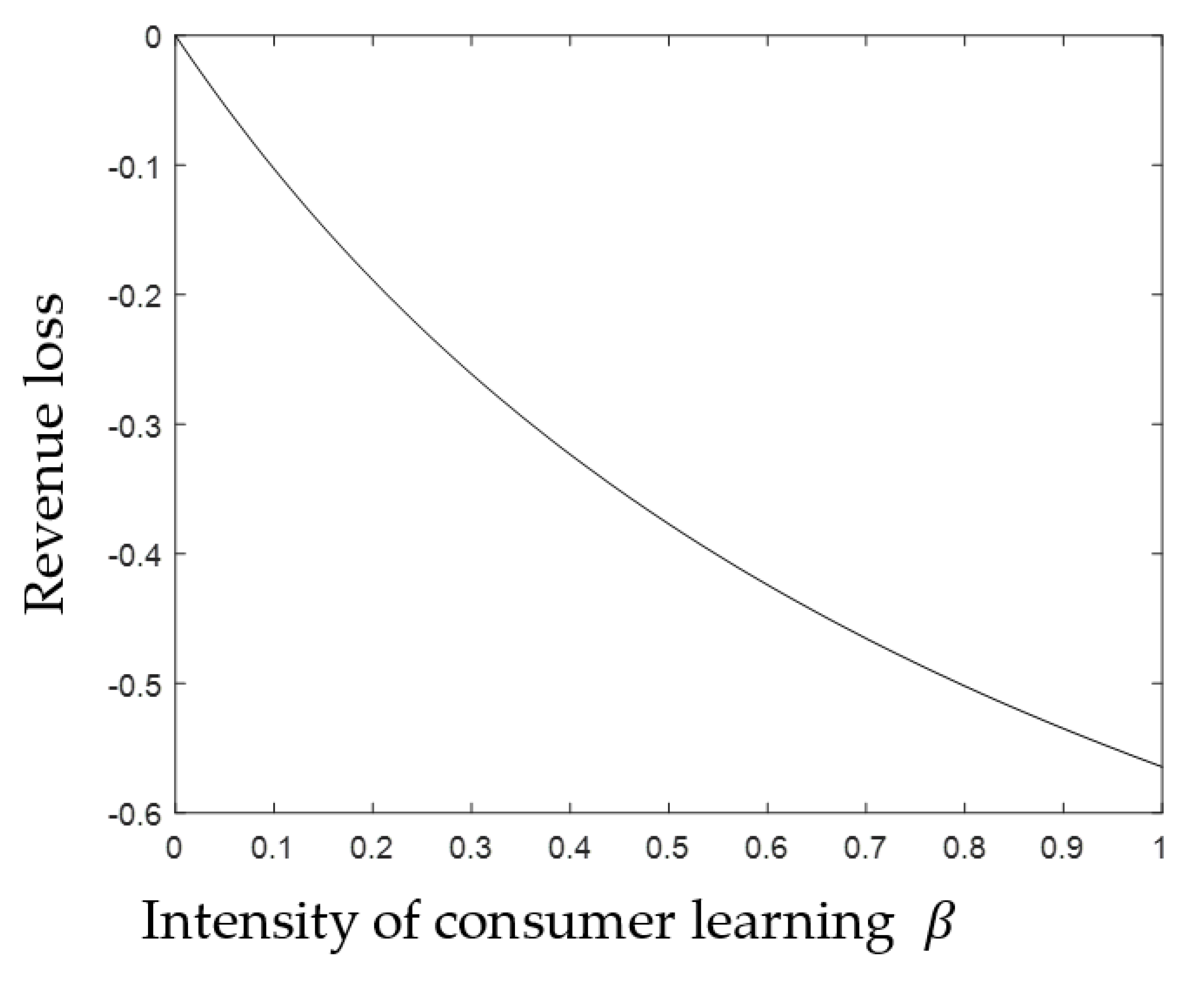
The intensity of consumer learning measures the degree to which consumers are affected by first-stage sales. In the benchmark model not considering consumers’ social learning, enterprises’ profits are not affected by learning intensity β . In the model considering consumers’ social learning, enterprises’ profits reduce with the increase in learning intensity   β . Therefore, enterprise’s revenue loss decreases monotonically with the increase in learning intensity   β .
Figure 4 describes how enterprise 0′s revenue loss varies with respect to consumer’s learning intensity β , when α = 0.6 , m = 2 . As the intensity of consumer learning increases, the competition between enterprises becomes stronger. No matter whether the enterprises are in a strong position or in a weak position in the market, the price they set will decrease with the increase in learning intensity, and their profits will also decrease with the increase in learning intensity.

6. Conclusions

Based on the classic Hotelling competition model, this study investigated a two-period pricing model of innovative product duopoly in consideration of consumers’ social learning. The optimal price decisions, maximum profits, and two-stage demands for enterprises were obtained. Then, the effect of consumers’ social learning on the prices and profits of competitive enterprises was studied through comparison with a benchmark model without social learning. Finally, the valuation gap between high- and low-quality products and the effect of consumer learning intensity were examined.
The main conclusions are as follows: (1) Consumers’ social learning will intensify competition between duopoly enterprises, which will lower their prices and profits. (2) The stronger the learning intensity of consumers, the greater the revenue loss of enterprises. The effect of the valuation gap between high-quality and low-quality products on enterprises’ revenue losses is non-monotonic.
There are a number of potential extensions that can be further studied. The first direction is a comparative analysis of preannounced pricing and responsive pricing strategies. Under a preannounced pricing strategy, each firm can vary its price from one period to another but needs to pre-commit to its price path before period 1. In this paper, the preannounced pricing strategy is adopted and the prices of period 1 and period 2 are assumed to be the same. Under a responsive pricing strategy, each firm can vary its price from one period to another without pre-commitment, i.e., the firm only needs to decide on its period 2 price at the beginning of period 2.
The second potential extension is considering a consumer learning mechanism driven by Bayesian inference. The existing literature on social learning can be broadly classified into two groups depending on the learning mechanism, either Bayesian or non-Bayesian. In Bayesian-driven learning mechanism, agents are rational and update their beliefs in a Bayesian way. They base their decisions only on the observed behavior of the previous agents and will ignore their own signals. Non-Bayesian learning mechanisms usually employ simpler and perhaps more plausible learning protocols, in which consumers exchange information about their experienced utility and use simple decision rules to choose between actions [24]. In this study, we employed a non-Bayesian learning mechanism; however, a consumer learning mechanism driven by Bayesian rule also deserves to be studied. Another scenario is that consumers in period 1 are able to discover the true qualities and channel the information to the period 2 consumers with some noise, so that period 2 consumers may have another means to update.
The third direction is that strategic consumers may choose to purchase at different times. For example, consumers in period 1 can strategically wait to purchase in period 2. As new experience goods, no consumer knows the true quality and valuation when the products are first introduced to the market. Therefore, some strategic consumers may wait for previous consumers’ product reviews and delay the purchase choice to period 2. Incorporating this strategic behaviors of consumers into the research will be very interesting.
The fourth potential extension is that each firm can endogenously choose its location on the Hotelling line before period 1. This study uses the classic Hotelling model and assumes the two enterprises are located at both ends of a linear city unit. In reality, firms can endogenously decide their locations on the Hotelling line before period 1. In this scenario, the demand functions of two products will be different from this paper.

Author Contributions

L.X.: Methodology, Validation, Formal analysis, Investigation, Writing—original draft, Visualization, Funding acquisition. H.Z.: Conceptualization, Software, Writing—original draft. Y.Q.: Writing —review and editing. All authors have read and agreed to the published version of the manuscript.

Funding

This research was funded by the National Natural Science Foundation of China (Nos. 71902041, 71801175) and Guangdong Basic and Applied Basic Research Foundation (No.2020A1515011511).

Acknowledgments

The authors thank the anonymous referees for their comments and suggestions.

Conflicts of Interest

The authors declare no conflict of interest.

Appendix A

Proof of Theorem 1.
Assume there is no difference between buying product 0 and product 1 for consumers located at x 1 . Therefore, consumers located at [ 0 ,   x 1 ] will choose to buy product 0, and consumers located at [ x 1 , 1 ] will choose to buy product 1.
v 0 + α m x 1 p 0 = v 0 + ( 1 α ) m ( 1 x 1 ) p 1 ,
x 1 = ( 2 α 1 ) m + p 1 p 0 2 + 1 2 .
The two enterprises’ profits are
π 0 = 2 x 1 p 0 ,
π 1 = 2 ( 1 x 1 ) p 1 .
Combine π 0 p 0 = 0 and π 1 p 1 = 0 , we can get:
p 0 * = 1 + ( 2 α 1 ) m 3 ,
p 1 * = 1 + ( 1 2 α ) m 3 ,
π 0 * = [ 3 + ( 2 α 1 ) m ] 2 9 ,
π 1 * = [ 3 + ( 1 2 α ) m ] 2 9 .
Proof of Theorem 2.
At period 1, there is no difference between buying product 0 and product 1 for consumers located at x 1 . Therefore, consumers located at [ 0 ,   x 1 ] will choose to buy product 0, and consumers located at [ x 1 , 1 ] will choose to buy product 1.
v 0 + α m x 1 p 0 = v 0 + ( 1 α ) m ( 1 x 1 ) p 1 ,
x 1 = ( 2 α 1 ) m + p 1 p 0 2 + 1 2 ,
Correspondingly, the demand of product 0 is x 1 = ( 2 α 1 ) m + p 1 p 0 2 + 1 2 , the demand of product 1 is   1 x 1 = ( 1 2 α ) m + p 0 p 1 2 + 1 2 .
At period 2, consumers can observe the demand of period 1 and update the probability α to α = α + β ( ( 2 α 1 ) m + p 1 p 0 2 + 1 2 α ) . At period 2, there is no difference between buying product 0 and product 1 for consumers located at x 2 .
v 0 + α m x 2 p 0 = v 0 + ( 1 α ) m ( 1 x 2 ) p 1 ,
x 2 = ( 2 α 1 ) ( 1 + β m β ) m + ( 1 + β m ) ( p 1 p 0 ) + 1 2 .
The two enterprises’ profits are
π 0 = ( x 1 + x 2 ) p 0 = [ 2 + ( 2 α 1 ) ( 2 + β m β ) m + ( 2 + β m ) ( p 1 p 0 ) 2 ] p 0 ,
π 1 = ( 2 x 1 x 2 ) p 1 = [ 2 + ( 1 2 α ) ( 2 + β m β ) m + ( 2 + β m ) ( p 0 p 1 ) 2 ] p 1 .
Combining π 0 p 0 = 0 and π 1 p 1 = 0 , we can get:
{ 2 + ( 2 α 1 ) ( 2 + β m β ) m + ( 2 + β m ) ( p 1 2 p 0 ) 2 = 0 2 + ( 1 2 α ) ( 2 + β m β ) m + ( 2 + β m ) ( p 0 2 p 1 ) 2 = 0 ,
p 0 * = 6 + ( 2 α 1 ) ( 2 + β m β ) m 3 ( 2 + β m ) ,
p 1 * = 6 + ( 1 2 α ) ( 2 + β m β ) m 3 ( 2 + β m ) .
6 ( 2 + β m β ) m > 0 must hold, so as to satisfy the non-negativity of product price. In equilibrium, the profits of enterprises are
π 0 * = [ 6 + ( 2 α 1 ) ( 2 + β m β ) m ] 2 18 ( 2 + β m ) ,
π 1 * = [ 6 + ( 1 2 α ) ( 2 + β m β ) m ] 2 18 ( 2 + β m ) .
Proof of Theorem 3.
In equilibrium, the demand of firm 0 at the first period and second period are
x 1 = ( 2 α 1 ) ( 2 + β m + 2 β ) m 6 ( 2 + β m ) + 1 2 ,
x 2 = ( 2 α 1 ) ( 2 + 3 β m 4 β + β 2 m 2 β 2 m ) m 6 ( 2 + β m ) + 1 2 .
It is easy to derive x 2 x 1 = ( 2 α 1 ) m β ( β m 2 β m 6 + 2 m ) 6 ( 2 + β m ) . According to the precondition of equilibrium,   β m 2 < 6 2 m + β m must hold. Therefore, β m 2 β m 6 + 2 m < 0 . From the above, we can know that x 2 x 1 > 0   holds when α < 1 2 ; x 2 x 1 = 0   holds when α = 1 2 ; x 2 x 1 < 0 holds when α > 1 2 . □
Proof of Theorem 4.
In equilibrium of the above two models,
p 0 * p 0 * = 6 + ( 2 α 1 ) ( 2 + β m β ) m 3 ( 2 + β m ) 1 ( 2 α 1 ) m 3 = ( 2 α + 2 ) β m 3 ( 2 + β m ) < 0 ,
p 1 * p 1 * = 6 + ( 1 2 α ) ( 2 + β m β ) m 3 ( 2 + β m ) 1 ( 1 2 α ) m 3 = ( 4 2 α ) β m 3 ( 2 + β m ) < 0 .
Proof of Theorem 5.
In equilibrium of the above two models,
  π 0 * π 0 * = [ 6 + ( 2 α 1 ) ( 2 + β m β ) m ] 2 18 ( 2 + β m ) [ 3 + ( 2 α 1 ) m ] 2 9 = β m { 6 ( 1 + 4 α ) m ( 1 2 α ) 2 [ 4 β 2 m + 2 β m m 2 β ] } 18 ( 2 + β m ) ,
π 1 * π 1 * = [ 6 + ( 1 2 α ) ( 2 + β m β ) m ] 2 18 ( 2 + β m ) [ 3 + ( 1 2 α ) m ] 2 9 = β m { 6 ( 5 4 α ) m ( 1 2 α ) 2 [ 4 β 2 m + 2 β m m 2 β ] } 18 ( 2 + β m ) .
We will prove this in two cases. When 4 2 m β ( m 1 ) 2 > 0 holds, obviously the numerator of π i * π i * is always less than zero, therefore π i * < π i * .
When 4 2 m β ( m 1 ) 2 < 0 holds, obviously m > 1 . With regard to π 0 * π 0 * , π 0 * π 0 * = β m { 6 ( 1 + 4 α ) + m ( 1 2 α ) 2 [ 4 + β + 2 m 2 β m + m 2 β ] } 18 ( 2 + β m ) β m 18 ( 2 + β m ) [ m ( 4 + β + 2 m 2 β m + m 2 β ) 6 ] ,
According to β m 2 < 6 2 m + β m , we have π 0 * π 0 * < β m 18 ( 2 + β m ) [ m ( 2 + β β m ) 6 ] = β m 18 ( 2 + β m ) ( 2 m + m β β m 2 6 ) .
According to 2 m < 6 + β m β m 2 , we have π 0 * π 0 * < β 2 m 3 9 ( 2 + β m ) ( 1 m ) .
From m > 1 , we can derive π 0 * π 0 * < 0 .
As for π 1 * π 1 * ,   π 1 * π 1 * = β m 18 ( 2 + β m ) { 6 ( 5 4 α ) + m ( 1 2 α ) 2 [ 4 + β + 2 m 2 β m + m 2 β ] } β m 18 ( 2 + β m ) [ m ( 4 + β + 2 m 2 β m + m 2 β ) 6 ] < 0 .
In sum, when considering consumers’ learning behavior, π i * < π i * . □

References

  1. Zhou, J.; Zhao, X.; Xue, L.; Gargeya, V. Double moral hazard in a supply chain with consumer learning. Decis. Support Syst. 2012, 54, 482–495. [Google Scholar] [CrossRef] [Green Version]
  2. Swinney, R. Selling to Strategic Consumers when Product Value is Uncertain: The Value of Matching Supply and Demand. Manag. Sci. 2011, 57, 1737–1751. [Google Scholar] [CrossRef] [Green Version]
  3. Feldman, P.; Papanastasiou, Y.; Segev, E. Social Learning and the Design of New Experience Goods. Manag. Sci. 2019, 65, 1502–1519. [Google Scholar] [CrossRef] [Green Version]
  4. Banerjee, A.V. A Simple Model of Herd Behavior. Q. J. Econ. 1992, 107, 797–817. [Google Scholar] [CrossRef] [Green Version]
  5. Banerjee, A.; Fudenberg, E. Word-of-mouth learning. Games Econ. Behav. 2004, 46, 1–22. [Google Scholar] [CrossRef]
  6. Chamley, C.P. Rational Herds: Economic Models of Social Learning; Cambridge University Press: Cambridge, UK, 2003; Volume 8, pp. 265–298. [Google Scholar]
  7. Gallego, G.; Wang, R.; Ward, J.; Hu, M.; Beltran, J.L. Flexible-Duration Extended Warranties with Dynamic Reliability Learning. Prod. Oper. Manag. 2014, 23, 645–659. [Google Scholar] [CrossRef]
  8. Kwon, H.D.; Xu, W.; Agrawal, A.; Muthulingam, S. Impact of Bayesian Learning and Externalities on Strategic Investment. Manag. Sci. 2016, 62, 550–570. [Google Scholar] [CrossRef]
  9. Çelen, B.; Kariv, S.; Schotter, A. An Experimental Test of Advice and Social Learning. Manag. Sci. 2010, 56, 1687–1701. [Google Scholar] [CrossRef] [Green Version]
  10. Acemoglu, D.; Dahleh, M.; Lobel, I.; Ozdaglar, A. Bayesian Learning in Social Networks. Rev. Econ. Stud. 2011, 78, 1201–1236. [Google Scholar] [CrossRef] [Green Version]
  11. Callander, S.; Hörner, J. The wisdom of the minority. J. Econ. Theory 2009, 144, 1421–1439.e2. [Google Scholar] [CrossRef]
  12. Song, Y. Social learning with endogenous observation. J. Econ. Theory 2016, 166, 324–333. [Google Scholar] [CrossRef]
  13. Yu, M.; Debo, L.; Kapuscinski, R. Strategic Waiting for Consumer-Generated Quality Information: Dynamic Pricing of New Experience Goods. Manag. Sci. 2016, 62, 410–435. [Google Scholar] [CrossRef]
  14. Petruzzi, N.C.; Dada, M. Dynamic pricing and inventory control with learning. Nav. Res. Logist. 2002, 49, 303–325. [Google Scholar] [CrossRef]
  15. Subramanian, U.; Rao, R.C. Leveraging Experienced Consumers to Attract New Consumers: An Equilibrium Analysis of Displaying Deal Sales by Daily Deal Websites. Manag. Sci. 2016, 62, 3555–3575. [Google Scholar] [CrossRef]
  16. Ovchinnikov, A.; Milner, J. Revenue Management with End?of?Period Discounts in the Presence of Customer Learning. Prod. Oper. Manag. 2011, 21, 69–84. [Google Scholar] [CrossRef]
  17. Allon, G.; Bassamboo, A. Buying from the Babbling Retailer? The Impact of Availability Information on Customer Behavior. Manag. Sci. 2011, 57, 713–726. [Google Scholar] [CrossRef] [Green Version]
  18. Papanastasiou, Y.; Savva, N. Dynamic Pricing in the Presence of Social Learning and Strategic Consumers. Manag. Sci. 2017, 63, 919–939. [Google Scholar] [CrossRef] [Green Version]
  19. Villas-Boas, J.M. Consumer Learning, Brand Loyalty, and Competition. Mark. Sci. 2004, 23, 134–145. [Google Scholar] [CrossRef]
  20. Villas-Boas, J.M. Dynamic Competition with Experience Goods. J. Econ. Manag. Strat. 2006, 15, 37–66. [Google Scholar] [CrossRef]
  21. Bergemann, D.; Välimäki, J. Dynamic Pricing of New Experience Goods. J. Polit. Econ. 2006, 114, 713–743. [Google Scholar] [CrossRef] [Green Version]
  22. Jing, B. Customer Recognition in Experience vs. Inspection Good Markets. Manag. Sci. 2015, 62, 216–224. [Google Scholar] [CrossRef]
  23. Jing, B. Social Learning and Dynamic Pricing of Durable Goods. Mark. Sci. 2011, 30, 851–865. [Google Scholar] [CrossRef]
  24. Crapis, D.; Ifrach, B.; Maglaras, C.; Scarsini, M. Monopoly Pricing in the Presence of Social Learning. Manag. Sci. 2017, 63, 3586–3608. [Google Scholar] [CrossRef] [Green Version]
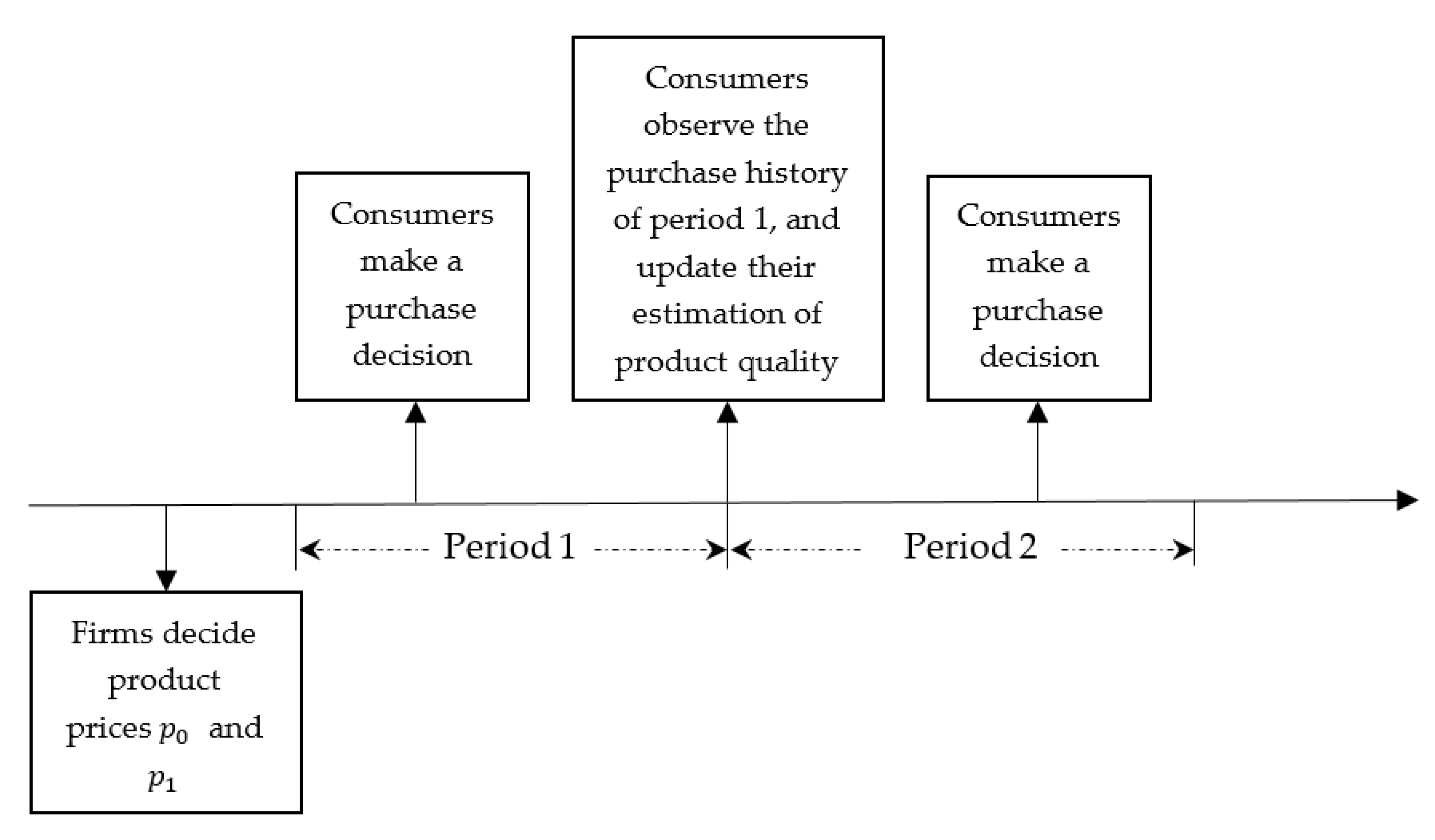
Figure 1. Decision-making process.
Sustainability 12 03806 g001
Figure 2. Decision-making process.
Sustainability 12 03806 g002
Figure 3. Effect of quality gap on enterprise’s revenue loss.
Sustainability 12 03806 g003
Figure 4. Effect of intensity of consumer learning on enterprise’s revenue loss.
Sustainability 12 03806 g004