Abstract
Even though biomass is characterised as renewable energy, it produces anthropogenic greenhouse gas (GHG) emissions, especially from biomass logistics. Lifecycle assessment (LCA) is used as a tool to quantify the GHG emissions from logistics but in the past the majority of LCAs have been steady-state and linear, when in reality, non-linear and temporal aspects (such as weather conditions, seasonal biomass demand, storage capacity, etc.) also have an important role to play. Thus, the objective of this paper was to optimise the environmental sustainability of forest biomass logistics (in terms of GHG emissions) by introducing the dynamic aspects of the supply chain and using the geographical information system (GIS) and agent-based modelling (ABM). The use of the GIS and ABM adds local conditions to the assessment in order to make the study more relevant. In this study, GIS was used to investigate biomass availability, biomass supply points and the road network around a large-scale combined heat and power plant in Naantali, Finland. Furthermore, the temporal aspects of the supply chain (e.g., seasonal biomass demand and storage capacity) were added using ABM to make the assessment dynamic. Based on the outcomes of the GIS and ABM, a gate-to-gate LCA of the forest biomass supply chain was conducted in order to calculate GHG emissions. In addition to the domestic biomass, we added imported biomass from Riga, Latvia to the fuel mixture in order to investigate the effect of sea transportation on overall GHG emissions. Finally, as a sensitivity check, we studied the real-time measurement of biomass quality and its potential impact on overall logistical GHG emissions. According to the results, biomass logistics incurred GHG emissions ranging from 2.72 to 3.46 kg CO2-eq per MWh, depending on the type of biomass and its origin. On the other hand, having 7% imported biomass in the fuel mixture resulted in a 13% increase in GHG emissions. Finally, the real-time monitoring of biomass quality helped save 2% of the GHG emissions from the overall supply chain. The incorporation of the GIS and ABM helped in assessing the environmental impacts of the forest biomass supply chain in local conditions, and the combined approach looks promising for developing LCAs that are inclusive of the temporal aspects of the supply chain for any specific location.
1. Introduction
Bioenergy is a crucial part of the energy system in Finland, for example, the share of woody biomass in primary energy was about 27% in 2017 [1]. The share of biomass in the energy mix is expected to increase in the future as Finland has pledged to end the use of coal by 2029 and biomass is considered to be the immediate solution to replace coal for energy production [2]. More biomass harvest means that transportation distances will also increase and since a significant part of Finnish small-diameter trees grow on peatlands, accessibility to energy wood will be more difficult [3].
In recent times, bioenergy has come under scrutiny for its environmental performance, even though it is considered to be a renewable source of energy [4]. Authorities around the world have imposed a variety of environmental policies that encourage organisations to conduct life cycle assessment (LCA), including greenhouse gas (GHG) mitigation. As in other fields, LCA is considered to be one of the best ways to quantify the environmental impacts and identify opportunities for improvement throughout the life cycle phases of bioenergy systems [5]. However, LCAs in the bioenergy sector are often steady-state and overly simplified, even though the supply chain is a complex system and dependent on multiple entities [6]. Furthermore, although LCA is the main tool used to quantify the environmental sustainability of biomass supply chains, very few studies have focused on its optimisation. A review study from 2014 by Cambero and Sowlati [7] found that none of the reviewed articles discussed the optimisation of environmental sustainability as a primary objective. Another review study from 2019 by Santos et al. [8] found that only three studies consideredoptimising the environmental sustainability of the biomass supply chain. Both reviews concluded that many optimisations focus on economic optimisation, and environmental sustainability is often an auxiliary objective coupled with the optimisation of economic sustainability.
Many studies have noted that the steady-state and linear nature of LCA is a major limitation and have explored the options to address this by introducing a dynamic approach using tools such as agent-based modelling (ABM) [6,9,10]. In addition to ABM, there are other tools available such as discrete-event simulation (DES) and system dynamics (SD) to assess the dynamic aspects of the biomass supply chain. However, ABM offers a unique opportunity to model the complexity of individual actors (agents) resulting from their individual actions and interactions with other agents in the real-world, which is either not readily available or not possible with DES or SD [11]. Kishita et al. [12] conducted a scenario analysis for a sustainable bioenergy business through a narrative storyline, which provides a consistent story as to what will happen to the business in the future. Aalto et al. [13] refers to this study by Kishita et al. as a way of using DES to assist with environmental impact assessment (CO2 emission calculation). However, the authors note that there are disadvantages to their approach since the study omits the ripple effects of the actions. The authors also point out that their approach is not dynamic in nature, especially in regard to the calculation of CO2 emissions. Halog and Manik [9] believe that the use of ABM and SD as a combined approach (also referred to as a hybrid approach) could identify the interaction of and between agents and help trace the potential pattern of dynamic supply chains. Some authors also believe that a hybrid approach can aid in exploring multiple “what if” scenarios for a particular system. Davis et al. [6] and Baustert and Benetto [14] suggest that ABM could be used to generate foreground data, also known as inventory, which could then be coupled with LCA. In addition to ABM, geographical information systems (GIS) are often used to analyse spatial information, which is important for collecting inventories in local contexts [15]. A review by Aalto et al. [13] suggests that there are multiple benefits of coupling GIS and ABM with LCA; however, their study found no research that combines all three modelling approaches. There are however, a number of studies that have coupled ABM with LCA in the bioenergy sector [6,16,17,18,19], and GIS with LCA [20,21,22].
1.1. The GIS
GIS is a tool used for the development, management, evaluation and presentation of data linked to the geographical (or spatial) setting. Most geospatial information can be reproduced for visualisation or evaluation in a presentable manner. In the 1990s, GIS was used primarily to evaluate the supply and transport expenses of biomass [23,24]. However, the range of research has subsequently been extended to include elements other than economics, such as improvements in land use or the environmental effects of biomass handling [25]. A significant benefit of GIS for biomass-supply studies is that GIS is able to optimise routes and calculate accurate travel distances, times and costs, even in complex supply schemes that include thousands of transport origins and multiple route choices.
1.2. ABM
ABM is a method of studying the activities of individuals (agents) and how they interact with each other in order to investigate a system. Because ABM is used in a broad spectrum of scientific fields, it has no specific definition. The agents serve as an abstract depiction of the true environment, while the model is the consequence of the mixed outcomes of individual agents’ choices. Each agent has its own features and characteristics, and because the system is dynamic it is possible to interconnect the properties of distinct agents as needed [6]. In bioenergy systems, agents may be a means of transportation (i.e., trucks, trains, and vessels), harvesters, forwarders, chippers, and users of the biomass such as power plants. ABM includes temporal changes in the study, allowing us to see the effects of time in the system. This also allows for the inclusion of the dynamic nature of the biomass supply system. Furthermore, ABM enables the generation of multiple scenarios with different initial conditions and agents’ decision-making logics.
1.3. LCA
LCA is a tool that is intended to evaluate the potential environmental effects of products or services. It is then used to recognise any opportunities to improve the environmental efficiency of a product or service at any stage of its life cycle. It can help decision-makers in the planning and design of products to enhance the environmental efficiency of products or services. LCA is also intended to be used as a marketing tool for any product or service to enable customers to create informed decisions about their choices. It has been used to estimate the environmental impact of consumer products since the 1960s and has been standardised by the International Organization for Standardization (ISO) since 1994 [26,27].
The LCA is conducted in four different but iterative phases, namely, goal and scope definition, life cycle inventory (LCI), life cycle impact assessment (LCIA), and interpretation. The system boundary and scope of the study are defined according to the aim of the project and the relevant information that falls within these boundaries are collected. In the impact assessment phase, the inventory is transformed into environmental impacts that they may have. Finally, in the interpretation stage, the outcomes of the inventory and impact-assessment stages are discussed, completed, and suggestions are made on the basis of the objectives identified in the first stage. In addition, these stages are iterative and can be adjusted to the scope of the research [28].
The primary aim of this study was to assess the GHG emissions of forest biomass logistics for a large-scale combined heat and power (CHP) plant in Finland. The concept was to use the GIS and ABM to incorporate the spatial and temporal aspects of the forest biomass supply chain. In the assessment, the GIS is used to analyse biomass availability, the accurate location of biomass supply points and travel distances with the route network, and ABM helped to assess the temporal aspects of the supply systems. The combination of the GIS and ABM provides real-world developments in a local context where biomass availability and logistics are dependent on variables such as weather, biomass demand in the region, forest biomass availability and accessibility, and forest owners’ willingness to sell biomass for energy. Consequently, the GIS and ABM were implemented to build an accurate inventory for the LCA of bioenergy logistics. In addition to the domestic biomass supply chain, the second aim of this study was to investigate potential GHG emissions resulting from the logistics of importing biomass to Finland. Finally, the third aim of the study was to assess the potential GHG benefits of the real-time measurement (RTM) of biomass quality at the power plant fuel-reception facility.
2. Materials and Methods
The GIS, ABM, and LCA were combined to assess the spatiotemporal aspects of the biomass supply chain and its global warming potential. The framework of the research is illustrated in Figure 1.
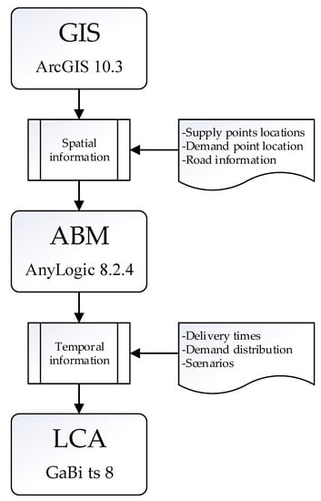
Figure 1.
The framework of the research.
2.1. GIS Assessment
The research was conducted using six baseline scenarios and three sensitivity scenarios (see Table 1). The “Domestic” scenario refers to biomass in Finland within a distance of 120 km from the power plant (see Figure 2) whereas the “Domestic and Imported” scenario also includes imported chips from Riga, Latvia (N 57°3′00″, E 24°5′00″). The share of imported biomass is ca. 7% of the total supplied biomass, and the amount of domestic biomass stays the same. The different amount of biomass in the Domestic and Domestic and Imported scenarios was used to assess additional impact. Wood chips from Riga were assumed to be collected from within a maximum distance of 100 km, and then brought to Naantali, Finland (N 60°27′37″, E 22°2′36″) on a vessel of 6300 m3.

Table 1.
Baseline and sensitivity scenarios with their abbreviations and supplied biomass in parentheses. Scenarios: AD (Domestic ‘A’), BD (Domestic ‘B’), CD (Domestic ‘C’), ADI (Domestic and imported ‘A’, BDI (Domestic and Imported ‘B’), CDI (Domestic and Imported ‘C’), BDRTM (Domestic ‘B’ with real time monitoring), and BDIRTM (Domestic and Imported ‘B’ with real time monitoring).
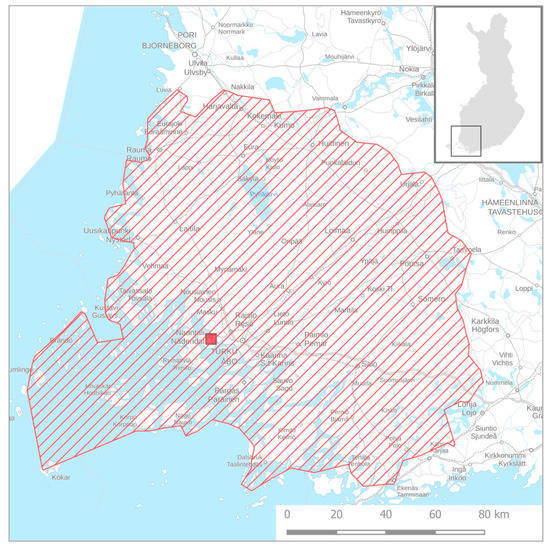
Figure 2.
Domestic biomass supply area around Naantali, Finland and the power plant location marked with a red square. Background map © National Land Survey of Finland, 2019, CC-BY 4.0.
Total harvest potential, accessibility, the probability of harvesting and the average forwarding distance to the nearest roadside (supply points) were assessed on a 2 km × 2 km grid using the ArcGIS version 10.3 software tool. In addition to the supply points, biomass demand by other plants in the region and forest owners’ willingness to sell biomass were also considered. For the simulation model, three main types of feedstock were considered: sawmill by-product (SB), imported wood chip (IWC) and domestic forest chip (DFC). The DFC type is further sub-classified into harvest residue (HR), stump (ST) and small-diameter whole tree or delimbed stem (WorD) feedstock. The share of different biomasses in the DFC feedstock is presented in Table 2.
Table 2.
Feedstock types: whole trees or delimbed stems (WorD), harvest residues (HR) and stump (ST).
There were 3883 supply points in the assessment with each containing an allocated proportion of the total harvest potential and harvest probability. For the simulation, 200 random rows were imported to the model. Then, the harvest potential was multiplied by 19.4 (i.e., 3883/200) to match the annual potential. The moisture content of WorD and HR were determined by harvest month. The moisture content (%) of biomass in each of the harvest months was taken from studies by Routa et al. [29] and Heiskanen et al. [30] and are presented in Supplementary Materials, Table S1. The moisture of ST feedstock was based on the empirical data [31], and in the model, it is determined by a triangular probability distribution where the most probable value is between 22.5% and 35%. The method for random selection and the harvest probability distribution have been reported by Aalto et al. [32]. The types of road and their average share in each scenario is presented in Supplementary Materials, Table S2. The average calorific values of feedstock in each scenario are presented in Supplementary Materials, Table S3.
2.2. Biomass Quality Measurement in Real-Time
As for the sensitivity scenarios, the FUELCONTROL® system was used to monitor the fuel quality in real-time before it is fed into the boiler at the power plant. A schematic flow diagram of supply chain is available in Supplementary Materials, Figure S1. RTM of fuel with X-ray technology has replaced the traditional sampling method, thus avoiding the manual job while enhancing energy production through efficient logistics. With the help of real-time information about biomass quality (e.g., moisture), biomass suppliers are able to avoid the repeated delivery of biomass with bad quality, which eventually improves the average quality of biomass at the plant yard storage facility [33].
2.3. ABM
ABM was used to consider the dynamic aspects of the supply chain and its individual entities. For example, with ABM, it is possible to model the individual properties of agents that affect their decisions. These decisions consider, for example, whether feedstock goes to a terminal or to the power plant, when to stop a delivery and when the feedstock can be acquired from roadside storage. In addition, ABM has the potential to track the state of different agents, which eventually helps to track the values for loading, unloading and driving (either empty or loaded). The detailed methodology used for simulation modelling, and the participating agents and their logics for the biomass supply system is described in Supplementary Materials, Section S2. The main agent has a map element that uses GIS to generate a road network that trucks and chippers use. Roadside, demand point, and terminal locations are set based on user-input coordinates and using the GIS. The model was built on AnyLogic Professional 8.2.4 and it is capable of doing a multi-year simulation with a refreshed supply for every year. Table 3 contains a brief description of each agent.
Table 3.
Biomass supply-chain agents and logics used for simulation.
The simulation is based on randomly selected supply points in a designated supply area. When a roadside dynamic event is triggered, fuel entities are created, and its moisture content is set. Fuel entities are moved to stand in a queue, where they are delayed to represent the drying at the stand. Moisture estimation models are used to change the fuel entities’ moisture and energy content during storage. After stand storage, fuel entities are moved to roadside storage and are stored there for a user-set time period. Again, moisture is estimated and after the storage period, a roadside storage state change is also available. At the start of a shift, a chipper looks for available roadside storage if it does not already have one selected. The chipper moves to the selected roadside storage location and then orders trucks. Trucks start their trip from the demand point if there is room in the storage at the demand point or if the terminal is enabled and there is room for fuel. The truck makes the trip to the roadside where the chipper is waiting. After arriving, the truck waits its turn for loading. In this event, both the chipper and truck agent must be present. After loading, the truck will go to the demand point to unload. If storage at the demand point is full, the truck will go to the terminal. The truck starts a new trip if there are more fuel entities to gather and if there is enough time in its shift. The schematic flowcharts regarding the logics of chippers and trucks are available in Supplementary Materials Figures S2 and S3, respectively. A complete decision logic is further illustrated in the Supplementary Materials, Figure S4.
2.4. LCA
The purpose of the LCA is to assess the environmental impact of the biomass supply chain to a large-scale CHP plant located in Naantali, Finland. The assessment is a gate-to-gate assessment, which means the starting point of the biomass is roadside storage near the forest and the end of the assessment is at the storage facility of the power plant. The LCA was conducted using the sustainability assessment software tool GaBi ts 8. GaBi is one of the most popular software tools available in the market for conducting an LCA. It has its own database incorporated into it and has a feature to integrate third-party databases such as Ecoinvent. The data regarding biomass availability in the forest and the distance to be covered by chippers and delivery trucks were assessed with GIS and ABM and these were used as a primary LCI for the LCA. Further inventory and their sources are presented in Table 4.
Table 4.
Unit processes—their description and sources.
The information from the LCI were then characterised to an impact category: “Global warming potential (GWP) 100 years excl. biogenic carbon dioxide” based on the guidelines of CML2001 (2016) [34], and presented with respect to the functional units of t CO2 eq. per year and kg CO2 eq. per MWh of wood fuel. The results from the impact assessment are interpreted in the discussion section.
3. Results
3.1. GIS and ABM Results
The results of GIS and ABM simulation for the monthly biomass supply and delivery distances are shown in Figure 3. According to the results, most biomass was delivered in January, followed by December and November. In other words, about 37% of the total biomass was delivered in those three months alone. On the other hand, the least amount of biomass was supplied in July, resulting in approximately 80% less delivery distance covered in July compared to January. There was no significant difference in delivery distance between AD and ADI, but in BD 17,000 km more distance was needed than in BDI. Similarly, CD needed 18,000 km more than its corresponding scenario, CDI.
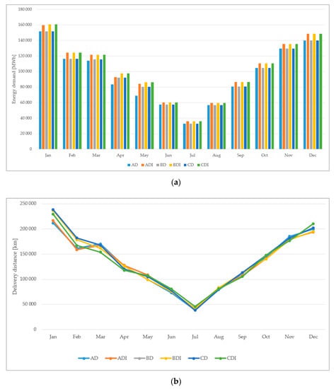
Figure 3.
Delivered biomass (a) and driving distance (b) for each month during a year for all six scenarios.
3.2. LCA Results
Figure 4 shows that ADI, BDI, and CDI have higher GHG emissions compared to their respective domestic scenarios with respect to both functional units. Furthermore, CDI has the highest GHG emissions for both functional units (4235 t CO2-eq per year and 3.46 kg CO2-eq per MWh), whereas AD has the lowest GHG emissions (3105 t CO2-eq per year and 2.72 kg CO2-eq per MWh) for both categories. On the other hand, imported biomass in the fuel mixture results in about 13% more emissions compared to the use of domestic biomass alone.
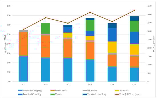
Figure 4.
Greenhouse gas (GHG) emissions for each scenario with respect to MWh and total emissions in a year.
Among the life cycle phases, the chipping operation and transportation are the major contributors to GHG emissions. In scenarios where imported biomass is in the fuel mix, vessel transportation becomes a major contributor as well.
3.3. Sensitivity Results
The impact of the RTM of biomass fuel at the fuel reception center at the power plant was studied with scenarios BD and BDI. According to Figure 5, the real-time fuel quality monitoring system helped to reduce the average moisture of WorD (by 2%) and ST (by 1%) in both BD and BDI scenarios.
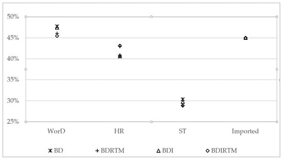
Figure 5.
The moisture content of biomass fuel at power plant storage facility with and without real-time measurement (RTM).
Because of adjustments to chipping and transportation activities that were led by feedback from the RTM system, 3.1% and 2.4% of transportation kilometers were saved in the BD and BDI scenarios, respectively. Consequently, as shown in Figure 6, RTM helped mitigate 2.7% and 2.1% of GHG emissions as compared to BD and BDI, respectively. The corresponding amount of GHG emissions mitigations were 92 t and 84 t per year from the studied product systems.
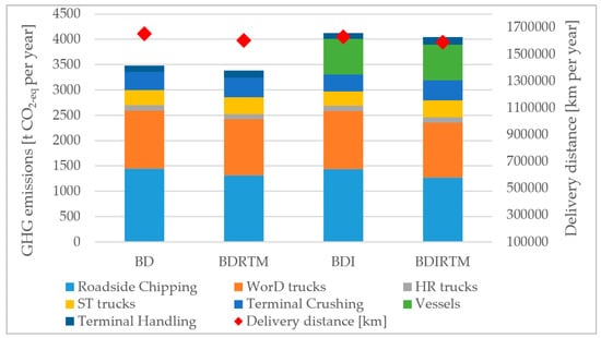
Figure 6.
Comparative delivery distances and GHG emissions with and without RMT in scenario B.
4. Discussion
This study investigated the environmental impact of forest biomass logistics for a large-scale CHP plant in Naantali, Finland in terms of GWP by means of GIS and the ABM. The GIS was used to analyse the local biomass supply points (forest roadside storage), the road network, the biomass terminal and power plant whereas ABM was used to simulate the supply system in a virtual environment. As a result, the amount of biomass and the potential delivery distances to the power plant or biomass terminal were identified for multiple scenarios with different biomass fuel fixture and supply systems. Based on those results, the existing literature, and databases, LCA was conducted using the GaBi ts modelling tool. The results show that the logistics of ST biomass has comparatively higher GHG emissions than WorD and HR, even though ST is comparatively drier than the other biomasses. Since stumps are crushed in a biomass terminal, terminal operations (such as crushing, handling, and transportation between terminal and power plant) make a significant difference to total GHG emissions. On the other hand, 7% imported biomass in the biomass fuel mixture—imported via sea transport from Riga to Naantali—results in 13% more GHG emissions.
The impact of continuous monitoring of feedstock quality at power plant reception facility was assessed as a sensitivity analysis. RTM technology was used to monitor the biomass quality (primarily moisture content) in real time, and with the help of this information, suppliers could select the best quality biomass (e.g., with lower moisture content) to be delivered to the power plant. As a consequence, the average moisture of the feedstock at the plant yard storage was reduced by about 2%. This is a significant reduction because the starting values of biomass supply points and the road network were the same in the main and sensitivity scenarios. In this regard, ABM was a convenient tool for investigating the effect of real-time information about the feedstock quality without having to conduct any field tests. Thus, we suggest that dynamic simulation tools are useful in determining the effects of new technologies in supply chains in a cost-effective way. However, simulations may not be completely flawless, and the results often require verification in the real world.
4.1. Uncertainty and Validation
In practice, simulation results are not 100% accurate and often need to be validated to some extent [38]. Aalto [39] believes that with reasonably accurate starting information and a working simulation model, one can expect results with reasonable accuracy. However, due to the lack of comparable real-world scenarios, simulation outcomes were not verified in this study. On the other hand, validation of LCA results is complicated and nearly impossible because LCAs are case specific and dependent on the assumptions and system boundaries of each study; thus, it is difficult to compare results. However, a study by Jäppinen et al. [40], wherein one of the scenarios spanned from forest roadside chipping to delivery to the user location in Finland, is similar to this study. According to their results, GHG emissions from biomass logistics vary from 2.05 to 2.69 g CO2-eq per MJ (or 7.38 kg to 9.6 kg CO2-eq per MWh) depending on the location of the supply area. The results are many times higher than the results of this study, but as mentioned earlier, one should consider the differences in assumptions made in both studies. For example, the supply area and biomass fuel mixture in the study by Jäppinen et al. [40] is different to this study. In addition, their studies did not include the temporal aspects of the supply chain (the dynamic simulation) and the results are only based on the resource availability and road network in a certain region of Finland.
4.2. The Dynamicity of LCA and Future Prospect
According to Baustert and Benetto [14], there are three ways to couple LCA and ABM based on the direction of information flow: ABM-enhanced LCA, LCA-enhanced ABM and ABM/LCA symbiosis (close-loop). Very few studies have considered the combination of ABM and LCA in the energy sector and none have considered it in the forest biomass supply chain. Gutierrez et al. [16] studied the evolution of Luxembourgish agriculture under multiple decision-making variables, such as economic incentives or environmental consciousness. Davis et al. [6] also combined LCA with dynamic simulation by feeding LCI into the ABM simulation. In that study, Davis et al. [6] concluded that the LCA itself is linear and steady-state because the simulation is not able to receive the feedback from LCA results and is not a closed-loop. Heairet et al. [17] studied the utilisation of switchgrass for multiple energy paths, such as ethanol or co-generation with coal. Their study combined ABM with LCA and defined it as ABM-enhanced LCA because it was fixed and was not a limiting factor in the simulation.
In this study, GIS and ABM were used to produce an LCI for the LCA of a biomass supply chain. For such an LCI, there were a multitude of variables such as biomass availability, weather, location, competing power plants, and forest owners’ willingness to sell the biomass, but those variables were effectively addressed at the GIS and ABM level, and the results were used as input information for the LCA. In retrospect, the LCA was a result of the spatiotemporal assessment but in itself, it was static and linear and not truly dynamic in nature. Nevertheless, the LCA results can be considered as close to the real-world scenarios. In other words, LCA was not a limiting variable for the simulation; however, LCA took full advantage of the dynamic nature of the agent-based simulation without being part of the simulation itself. In future research, one alternative could be to include the emission factors of the desired impact categories as one of the agents for the simulation. In this way, LCA results could be attributed to other variables and the results can be further classified according to the limiting factors for LCA as well. This close-loop combination of LCA and ABM may potentially be a better way to achieve a truly dynamic LCA.
5. Conclusions
The temporal aspects of biomass supply chains are often neglected in LCAs even though they have a crucial role to play. This paper combined LCA with spatial and temporal aspects of a forest biomass supply chain using GIS and ABM, respectively. The use of a combined approach offers results with respect to local conditions and temporal variables. Furthermore, the ABM offers an optimisation opportunity for linear LCAs, and subsequently, for the environmental sustainability of bioenergy. In future, researchers could use a close-loop combination of LCA and ABM to achieve true dynamicity, particularly for LCA.
Supplementary Materials
Additional file available at https://www.mdpi.com/2071-1050/12/5/1964/s1: Figure S1. A schematic flow diagram of biomass flow with and without RTM. Figure S2. Chipper agent state chart. Figure S3. A truck agent’s state chart. Figure S4. A flowchart of the truck and chipper logic used in the model. Figure S5. A flowchart of the stump truck logic used in the model. Table S1. The moisture content of biomasses at a forest roadside. Table S2. Road types and their share in different scenarios. Table S3. Biomass properties in different scenarios.
Author Contributions
Conceptualisation, R.K.C.; methodology, R.K.C., M.A. and O.-J.K.; software, R.K.C., M.A. and O.-J.K.; writing—original draft preparation, R.K.C.; writing—review and editing, R.R.C., M.A., O.-J.K., T.R., and S.P.; supervision, T.R. All authors have read and agreed to the published version of the manuscript.
Funding
This research received no external funding.
Conflicts of Interest
The authors declare no conflict of interest.
References
- Finnish Statistics. Finnish Statistics: Total Energy Consumption by Source. Available online: https://www.stat.fi/til/ehk/2018/01/ehk_2018_01_2018-06-27_tie_001_en.html (accessed on 9 February 2019).
- Ministry of Economic Affairs and Employment. Legislative Proposals: Coal Ban in 2029, More Transport Biofuels and More Biofuel Oil for Heating and Machinery. Available online: https://tem.fi/en/article/-/asset_publisher/lakiehdotukset-kivihiilikielto-2029-lisaa-biopolttoaineita-liikenteeseen-seka-biopolttooljya-lammitykseen-ja-tyokoneisiin (accessed on 8 August 2019).
- Anttila, P.; Nivala, V.; Salminen, O.; Hurskainen, M.; Kärki, J.; Lindroos, T.J.; Asikainen, A. Regional Balance of Forest Chip Supply and Demand in Finland in 2030. Silva Fennica 2018, 52. [Google Scholar] [CrossRef]
- Vanhala, P.; Repo, A.; Liski, J. Forest Bioenergy at the Cost of Carbon Sequestration? Curr. Opin. Environ. Sustain. 2013, 5, 41–46. [Google Scholar] [CrossRef]
- Cherubini, F.; Strømman, A.H. Life Cycle Assessment of Bioenergy Systems: State of the Art and Future Challenges. Bioresour. Technol. 2011, 102, 437–451. [Google Scholar] [CrossRef] [PubMed]
- Davis, C.; Nikolić, I.; Dijkema, G.P.J. Integration of Life Cycle Assessment into Agent-Based Modeling. J. Ind. Ecol. 2009, 13, 306–325. [Google Scholar] [CrossRef]
- Cambero, C.; Sowlati, T. Assessment and Optimization of Forest Biomass Supply Chains from Economic, Social and Environmental Perspectives—A Review of Literature. Renew. Sustain. Energy Rev. 2014, 36, 62–73. [Google Scholar] [CrossRef]
- Santos, A.; Carvalho, A.; Barbosa-Póvoa, A.P.; Marques, A.; Amorim, P. Assessment and Optimization of Sustainable Forest Wood Supply chains–A Systematic Literature Review. For. Policy Econ. 2019, 105, 112–135. [Google Scholar] [CrossRef]
- Halog, A.; Manik, Y. Advancing Integrated Systems Modelling Framework for Life Cycle Sustainability Assessment. Sustainability 2011, 3, 469–499. [Google Scholar] [CrossRef]
- Marvuglia, A.; Gutiérrez, T.N.; Baustert, P.; Benetto, E. Implementation of Agent-Based Models to Support Life Cycle Assessment: A Review Focusing on Agriculture and Land Use. AIMS Agric. Food 2018, 3, 535–560. [Google Scholar] [CrossRef]
- Siebers, P.; Macal, C.M.; Garnett, J.; Buxton, D.; Pidd, M. Discrete-Event Simulation is Dead, Long Live Agent-Based Simulation! J. Simul. 2010, 4, 204–210. [Google Scholar]
- Kishita, Y.; Nakatsuka, N.; Akamatsu, F. Scenario Analysis for Sustainable Woody Biomass Energy Businesses: The Case Study of a Japanese Rural Community. J. Clean. Prod. 2017, 142, 1471–1485. [Google Scholar] [CrossRef]
- Aalto, M.; Raghu, K.; Korpinen, O.; Karttunen, K.; Ranta, T. Modeling of Biomass Supply System by Combining Computational methods–A Review Article. Appl. Energy 2019, 243, 145–154. [Google Scholar]
- Baustert, P.; Benetto, E. Uncertainty Analysis in Agent-Based Modelling and Consequential Life Cycle Assessment Coupled Models: A Critical Review. J. Clean. Prod. 2017, 156, 378–394. [Google Scholar] [CrossRef]
- Santibañez-Aguilar, J.E.; Flores-Tlacuahuac, A.; Betancourt-Galvan, F.; Lozano-García, D.F.; Lozano, F.J. Facilities Location for Residual Biomass Production System using Geographic Information System Under Uncertainty. ACS Sustain. Chem. Eng. 2018, 6, 3331–3348. [Google Scholar]
- Gutiérrez, T.N.; Rege, S.; Marvuglia, A.; Benetto, E. Introducing LCA results to ABM for assessing the influence of sustainable behaviours. In Trends in Practical Applications of Agents, Multi-Agent Systems and Sustainability; Springer: Berlin/Heidelberg, Germany, 2015; pp. 185–196. [Google Scholar]
- Heairet, A.; Choudhary, S.; Miller, S.; Xu, M. Beyond Life Cycle Analysis: Using an Agent-Based Approach to Model the Emerging Bio-Energy Industry. In Proceedings of the 2012 IEEE International Symposium on Sustainable Systems and Technology (ISSST), Boston, MA, USA, 16–18 May 2012; pp. 1–5. [Google Scholar]
- Lan, K.; Yao, Y. Integrating Life Cycle Assessment and Agent-Based Modeling: A Dynamic Modeling Framework for Sustainable Agricultural Systems. J. Clean. Prod. 2019, 238, 117853. [Google Scholar] [CrossRef]
- Wu, S.R.; Li, X.; Apul, D.; Breeze, V.; Tang, Y.; Fan, Y.; Chen, J. Agent-Based Modeling of Temporal and Spatial Dynamics in Life Cycle Sustainability Assessment. J. Ind. Ecol. 2017, 21, 1507–1521. [Google Scholar]
- Jäppinen, E.; Korpinen, O.; Ranta, T. The Effects of Local Biomass Availability and Possibilities for Truck and Train Transportation on the Greenhouse Gas Emissions of a Small-Diameter Energy Wood Supply Chain. Bioenergy Res. 2013, 6, 166–177. [Google Scholar] [CrossRef]
- Mirkouei, A.; Haapala, K.R.; Sessions, J.; Murthy, G.S. A Mixed Biomass-Based Energy Supply Chain for Enhancing Economic and Environmental Sustainability Benefits: A Multi-Criteria Decision Making Framework. Appl. Energy 2017, 206, 1088–1101. [Google Scholar] [CrossRef]
- Sánchez-García, S.; Athanassiadis, D.; Martínez-Alonso, C.; Tolosana, E.; Majada, J.; Canga, E. A GIS Methodology for Optimal Location of a Wood-Fired Power Plant: Quantification of Available Woodfuel, Supply Chain Costs and GHG Emissions. J. Clean. Prod. 2017, 157, 201–212. [Google Scholar]
- Noon, C.E.; Daly, M.J. GIS-Based Biomass Resource Assessment with BRAVO. Biomass Bioenergy 1996, 10, 101–109. [Google Scholar] [CrossRef]
- Zhang, F.; Johnson, D.M.; Sutherland, J.W. A GIS-Based Method for Identifying the Optimal Location for a Facility to Convert Forest Biomass to Biofuel. Biomass Bioenergy 2011, 35, 3951–3961. [Google Scholar]
- Malczewski, J. GIS-Based Land-use Suitability Analysis: A Critical Overview. Prog. Plan. 2004, 62, 3–65. [Google Scholar] [CrossRef]
- Guinee, J.B.; Heijungs, R.; Huppes, G.; Zamagni, A.; Masoni, P.; Buonamici, R.; Ekvall, T.; Rydberg, T. Life Cycle Assessment: Past, Present, and Future. Environ. Sci. Technol. 2011, 45, 90–96. [Google Scholar] [CrossRef] [PubMed]
- McManus, M.C.; Taylor, C.M. The Changing Nature of Life Cycle Assessment. Biomass Bioenergy 2015, 82, 13–26. [Google Scholar] [CrossRef]
- Standardoimisliitto, S. Standardi SFS-EN ISO 14040. Ympäristöasioiden Hallinta. Elinkaariarviointi. Periaatteet Pääpiirteet [ISO 14044:2006 Environmental Management—Life Cycle Assessment—Requirements and Guidelines]; ISO: Geneva, Switzerland, 2007. [Google Scholar]
- Routa, J.; Kolström, M.; Ruotsalainen, J.; Sikanen, L. Validation of Prediction Models for Estimating the Moisture Content of Small Diameter Stem Wood. Croat. J. For. Eng. J. Theory Appl. For. Eng. 2015, 36, 283–291. [Google Scholar]
- Heiskanen, V.; Raitila, J.; Hillebrand, K. Varastokasassa Olevan Energiapuun Kosteuden Muutoksen Mallintaminen [Modeling of Moisture Change in Energy Wood in a Storage]; VTT-R-08637-13; VTT: Jyväskylä, Finland, 2014. [Google Scholar]
- Muinonen, M. (Inray Oy, 50130 Mikkeli, Finland). Moisture Content of Stumps, Inray.fi. Personal communication, 2019. [Google Scholar]
- Aalto, M.; Korpinen, O.; Ranta, T. Feedstock Availability and Moisture Content Data Processing for Multi-Year Simulation of Forest Biomass Supply in Energy Production. Silva Fenn. 2019, 53. [Google Scholar] [CrossRef]
- Inray Ltd. FUELCONTROL®: Efficient Energy Production. Available online: www.Inray.fi (accessed on 9 February 2019).
- CML. CML-IA Characterisation Factors; Leiden University: Leiden, The Netherlands, 2016; Volume 2019. [Google Scholar]
- Werner, F. Wood Chipping, Mobile Chipper at Forest Road. Ecoinvent 2012, 3. [Google Scholar]
- Ovaskainen, H. CO2-Eq Emissions and Energy Efficiency in Forest Biomass Supply Chains—Impact of Terminals; Metsäteho Publication Series 4b/2017; Metsäteho: Vantaa, Finland, 2017. [Google Scholar]
- GaBi Databases. Thinkstep AG (Formerly PE INTERNATIONAL AG); LBP-GaBi, University of Stuttgart: Leinfelden-Echterdingen, Germany, 2009. [Google Scholar]
- Robinson, S. Conceptual Modelling for Simulation Part I: Definition and Requirements. J. Oper. Res. Soc. 2008, 59, 278–290. [Google Scholar] [CrossRef]
- Aalto, M. Agent-Based Modeling as Part of Biomass Supply System Research. Ph.D. Thesis, Lappeenranta-Lahti University of Technology LUT, Lappeenranta, Finland, 2019. [Google Scholar]
- Jäppinen, E.; Korpinen, O.; Ranta, T. GHG Emissions of Forest-biomass Supply Chains to Commercial-scale Liquid-biofuel Production Plants in F Inland. GCB Bioenergy 2014, 6, 290–299. [Google Scholar] [CrossRef]
© 2020 by the authors. Licensee MDPI, Basel, Switzerland. This article is an open access article distributed under the terms and conditions of the Creative Commons Attribution (CC BY) license (http://creativecommons.org/licenses/by/4.0/).