Predicting the Water-Conducting Fracture Zone (WCFZ) Height Using an MPGA-SVR Approach

Abstract

Mine water that inrushes from coal-roof strata has always posed a substantial threat to mining activities every year. Therefore, an accurate prediction of the water-conducting fracture zone (WCFZ) height in the mining overburden strata is of great significance for the prevention and control of mine water accidents. The support vector regression (SVR) is proposed to predict the height of the WCFZ based on the mining depth, hard rock proportional coefficient, mining thickness and length of the working face. Simultaneously, the multi-population genetic algorithm (MPGA) is employed to search for the optimal SVR parameters. The MPGA-SVR model is trained and tested with a total of 69 collected data samples, and it is also applied to a field test. The accuracy and stability of the model were measured by the mean squared error and correlation coefficients. The obtained results show that the MPGA-SVR model achieves a higher accuracy and stability than the traditional empirical formula and genetic algorithm (GA)-SVR model. In terms of the process for optimizing the SVR parameters, the MPGA can find the optimal parameters more quickly and accurately, and it can effectively overcome the problem of premature and slow convergence of the genetic algorithm (GA). The proposed model improves the prediction accuracy and stability, which will help to avoid accidents caused by the inrush of water inrush in mining overburden strata and protect the ecological environment of the mining area.

1. Introduction

As an important fossil energy source, coal has always played a dominant role in China’s primary energy consumption structure [1,2]. Although the safety situation of coal mines has been improved in recent years, mine water has always been a substantial threat to mining safety [3]. In the process of mining activities, the equilibrium state of the original rock stress in the overburden strata is destroyed, which leads to collapse, fracture and bending in the mining overburden strata. Once these fractures are interconnected with a water-bearing body (surface water, goaf water or aquifer water) in the mining overburden strata, the mine water will flow into the working face and bring huge economic losses and casualties, as illustrated in Figure 1 [4]. With the increase of mining depths, mining intensity and mining speed, the problem of mine water is becoming more prominent [5]. Therefore, accurately predicting the height of the water-conducting fracture zone (WCFZ) in the mining overburden strata is of great significance for the safe production of coal mining [6,7,8].

In the process of coal mining, the development of a WCFZ in mining overburden strata is an extremely complicated mechanical problem, which is characterized by the fuzzy randomness of the rock stratum structure, the complexity of the mining influence stress change and the nonlinear deformation and failure of the mining overburden. To predict the height of the WCFZ, scholars have proposed many methods, such as the field measurement method [9,10], theoretical calculations, numerical simulations [11,12,13], empirical formulas [14] and intelligence algorithms [15]. Among them, the field measurement method has the highest accuracy, but it is time consuming, laborious and costly [16]. The theoretical calculation method is too idealistic and has a large deviation from the actual complex geological conditions. The accuracy of the numerical simulation method is closely related to the geological condition parameters of the model, and the accurate acquisition of these parameters is difficult. The empirical formula considers a single influencing factor that is insufficient to reflect the combined effects of multiple influencing factors [3,17]. Increasingly more methods have been proposed with the deepening of research, and the prediction results of each method often have large differences since each method has a different level of adaptability and constraints.

In recent years, with the development and promotion of artificial intelligence technology, some machine learning methods, such as artificial neural networks (ANNs), decision trees (DTs) and support vector regression (SVR), have been developed. These methods have the advantages of comprehensive consideration, simple operation, low cost and good prediction results, therefore they are introduced to predict the height of the WCFZ. Ma et al. (2008) [18] established a three-layer Back Propagation (BP) neural network for predicting the height of the water-conducting fracture zone, and the prediction results are more reasonable and accurate than those of the empirical formula. Q. Wu et al. (2017) [19] presented a radial basis function neural network (RBFNN) model to predict the height of the WCFZ in a fully mechanized longwall mining operation with sublevel caving. However, the ANN is not stable enough to make a prediction with a small data sample, and the final prediction result easily falls into a local optimal solution since the parameters are often solved by a gradient technique. Zhang et al. (2017) [10] proposed a random forest regression model that is applied to the Hongliu Coal Mine in Northwest China with a high prediction accuracy. However, this model takes much time and has a high calculation cost, and the model is prone to over-fitting when the sample set is noisy.

The SVR is a machine learning method based on statistical learning theory and structural risk minimization criteria, which can be applied to small data sample for learning and predicting [20]. The SVR has the advantages of high accuracy, fast convergence speed and strong generalization ability, and it is widely used for predictions [21,22,23]. On the other hand, the setting of the SVR model parameters directly affects the performance of the model, and the problem of setting the model parameters is still not well solved [17]. Sun et al. (2009) [24] and Roushangar et al. (2015) [25] proposed a hybrid calculation system in which genetic algorithm (GA) was adopted to search for the SVR parameters, and the results were encouraging. As a method to search for the optimal solution by simulating the natural evolution process, GA was first proposed by Holland (1975) [26]. Although the GA has inherent implicit parallelism and better global optimization ability, many shortcomings have also been exposed with the wide application of GA and the deepening of research. In the GA evolution process, the choice of the crossover and mutation probability often determines the global search performance of the algorithm and the balance with the local search ability. In the actual application process, the value of the crossover and mutation probability are often fixed. There is a risk of premature convergence. The individuals in the group prematurely move towards a unified state and gradually stop evolving, therefore the result is a local optimum rather than a global optimum. On the other hand, the GA also has the disadvantage of slow convergence; that is, it fluctuates as it approaches the optimal solution but does not converge quickly. To deal with this problem, the concept of information theory has been introduced to preventing from premature convergence. Information-guided mutation was performed on multiple variables, and selection was made based on the obtained information entropy [27]. In addition, there are also optimization designs based on single genetic algorithm to reduce the probability of premature convergence. The main reason for the premature and slow convergence of the GA is that the population loses diversity before the optimal solution (or satisfactory solution) is obtained during the population evolution. To make full use of the global evolutionary characteristics of the GA and avoid its shortcomings, the multi-population genetic algorithm (MPGA) is first adopted to establish an MPGA-SVR model for predicting the height of the WCFZ. For the proposed model, this paper analyses its prediction performance in terms of accuracy and stability. The empirical formula and GA-SVR were also adopted to predict the height for comparison.

2. Methods

2.1. Support Vector Regression (SVR)

The SVR is an application model of a support vector machine (SVM), which was proposed by Vapnik (2000) [28]. The SVR model transforms complex low-dimensional non-linear regression problems into linear regression problems in high-dimensional feature space by applying a mapping function, Φ(x). The regression function is defined as follows [29]:

$$f\left(x\right)=\omega \cdot \mathsf{\Phi }\left(x\right)+b$$

(1)

where $\omega$ is the weight, is the threshold, Φ(x) is the inner product. The Equation (1) can be transformed into the following functional minimum problem:

$$\{\begin{array}{l}R\left(\omega \right)=\min \left[\frac{1}{2}{\Vert \omega \Vert }^2+C{\displaystyle \sum _{i=1}^k\left({\xi }_i+{\xi }_i^{\ast }\right)}\right]\\ s.t.\{\begin{array}{l}\omega \cdot \mathsf{\Phi }\left(x_i\right)+b-y_i\le \epsilon +{\xi }_i\\ y_i-\omega \cdot \mathsf{\Phi }\left(x_i\right)-b\le \epsilon +{\xi }_i^{\ast }\\ {\xi }_i\ge 0,{\xi }_i^{\ast }\ge 0\end{array}\end{array}$$

(2)

where x_i and y_i is respectively the input and output values of the training samples, $\epsilon$ is the insensitive loss function parameter, $\xi$ and ${\xi }^{\ast }$ are the two sets of non-negative relaxation variables, C is the penalty factor.

Equation (2) can be transformed into a dual problem by the Lagrangian multiplier method:

$$\{\begin{array}{l}J\left({\alpha }_i,{\alpha }_i^{\ast }\right)=\max [{\displaystyle \sum _{i=1}^k\left({\alpha }_i^{\ast }-{\alpha }_i\right)}{y}_i-\epsilon {\displaystyle \sum _{i=1}^k\left({\alpha }_i^{\ast }+{\alpha }_i\right)}{y}_i-\frac{1}{2}{\displaystyle \sum _{i=1}^k{\displaystyle \sum _{j=1}^k\left({\alpha }_i^{\ast }-{\alpha }_i\right)\left({\alpha }_i^{\ast }-{\alpha }_i\right)\left(\mathsf{\Phi }\left(x_i\right)\cdot \mathsf{\Phi }\left(x_j\right)\right)}}]\\ s.t.\{\begin{array}{l}{\displaystyle \sum _{i=1}^k\left({\alpha }_i^{\ast }-{\alpha }_i\right)=}0\\ {\alpha }_i,{\alpha }_i^{\ast }\in \left[0,C\right]\end{array}\end{array}$$

(3)

By solving Equation (3), the SVR regression function can be obtained as shown in Equation (4):

$$f\left(x\right)={\displaystyle \sum _{i=1}^k\left({\alpha }_i-{\alpha }_i^{\ast }\right)K\left(x_i,x_j\right)}+b$$

(4)

where the K(x_i, x_j) is the kernel function of SVR. As different kernel functions have different kernel function parameters, and the most commonly used Gaussian Radial Basis (RBF) kernel function [30] as shown in Equation (5) is selected in this paper:

$$K\left(x_i,x_j\right)=\exp \left[-\frac{{\Vert x_i-x_j\Vert }^2}{2{\sigma }^2}\right]$$

(5)

where $\sigma$ is the only adjustable kernel width parameter in the RBF function.

If $g=1/2{\sigma }^2$, then there are three parameters (C, $\epsilon$, g) in the SVR regression function that need to be determined. The insensitive loss coefficient $\epsilon$ controls the width of the insensitive region of the regression function to the sample data and affects the number of support vectors. If the value of $\epsilon$ is too large, the number of support vectors will be small, which may cause the model to be too simple and the learning accuracy is not enough. If the value of $\epsilon$ is too small, the regression accuracy is high, but it may cause the model to be too complicated and the generalization ability is poor. The penalty coefficient C reflects the penalty degree of the algorithm on sample data beyond $\epsilon$, and its value affects the complexity and stability of the model. If the value of C is too small, the penalty for the sample data exceeding $\epsilon$ is small, and the training error becomes large. If the value of C is too large, the learning accuracy is high, but the generalization ability of the model is poor. The kernel width parameter $\sigma$ reflects the degree of correlation between support vectors. If $\sigma$ is too small, the relationship between support vectors is loose, the learning machine is relatively complicated and the promotion ability cannot be guaranteed. If $\sigma$ is too large, the influence between support vectors is too strong, and it is difficult for the regression model to achieve sufficient accuracy.

From the above analysis, the complexity and generalization ability of the SVR model depends on these three parameters. It is unreasonable and time-consuming to optimize and select each parameter individually in the parameter selection. These three parameters should be considered simultaneously. Therefore, it is very important to find an accurate, stable and fast parameter selection method. It is difficult to obtain satisfactory results by directly using the default parameters or simply using the Cross Validation (CV) method provided by the LibSVM toolbox in Matlab to optimize the parameters in the SVR model. In this paper, the MPGA is employed to optimize the parameters in the SVR model.

2.2. The Multi-Population Genetic Algorithm (MPGA)

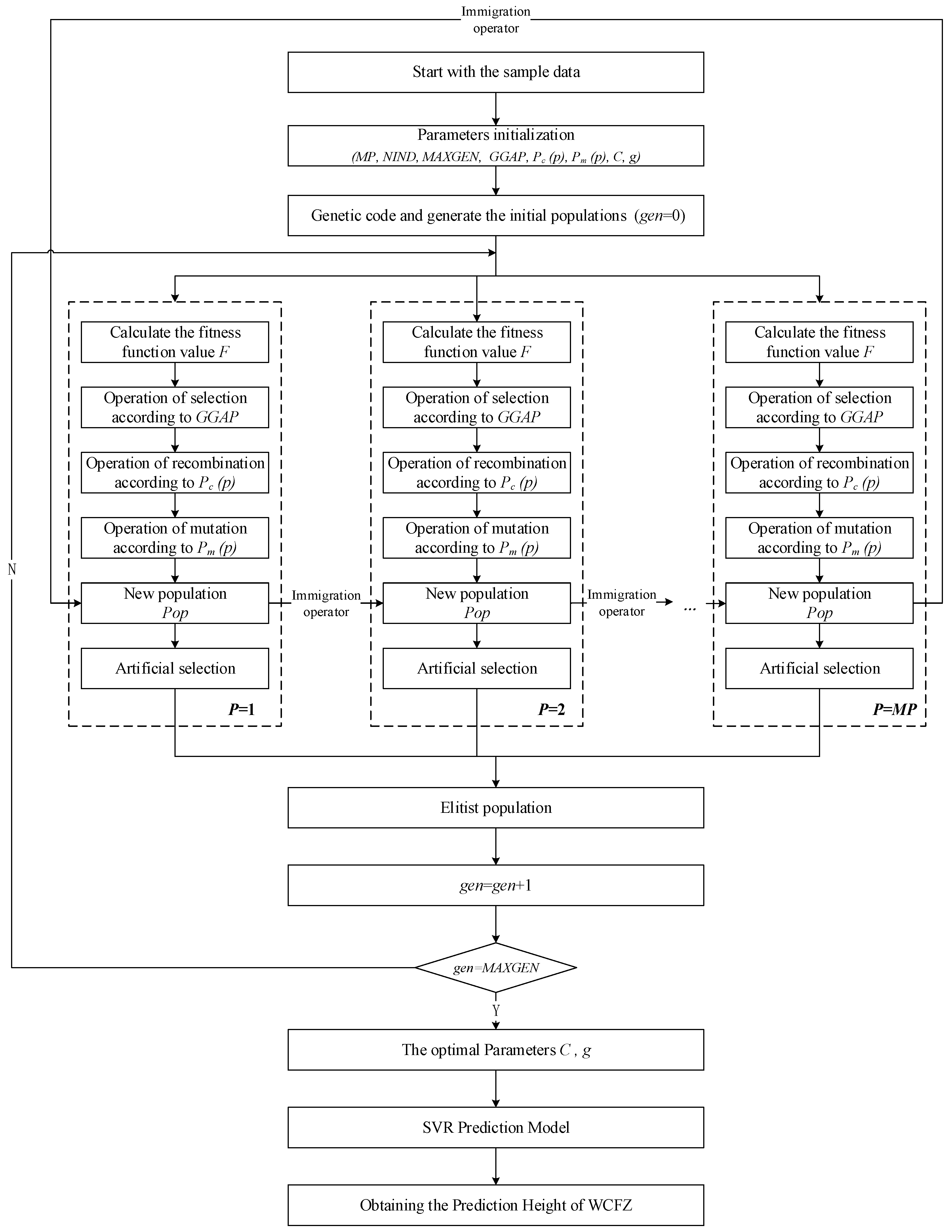
The MPGA is an improvement based on the GA, which can well solve the premature convergence and slow convergence of the GA. In the process of GA evolution, the selection of crossover probability (Pc) and mutation probability (Pm) often determines the global search of the algorithm and the balance of local search ability. The crossover operator is the main operator for generating new individuals, which determines the ability of genetic algorithm to search globally. The mutation operator is only the auxiliary operator that generates the new individual, which determines the local search ability of the genetic algorithm. Many scholars [31,32,33] recommend choosing a larger Pc (0.7–0.9) and a smaller Pm (0.001–0.05). However, there are still many values for Pc and Pm. For different choices, the optimization results are quite different. The MPGA compensates for this shortcoming of GA by co-evolution of several populations with different control parameters, taking into account both global search and local search of the algorithm.

In the evolution of MPGA, the various independent populations are connected by immigration operators. The immigration operator introduces the optimal individuals that appear in the evolution process of various populations periodically (this article sets every other generation) into other populations, and realizes the information exchange between the populations [34]. The specific operational rule is to replace the worst individual in the target population with the best individual in the source population. After each generation of evolution is completed, the best individuals in each population are selected by the artificial selection operator and placed in the elite population for preservation. The elite population does not perform genetic operations such as crossover and mutation to ensure that the optimal individuals produced by various groups in the evolution process are not destroyed or lost [35]. Based on GA, the MPGA co-evolve by introducing multiple populations with different control parameters to shorten the generation number needed to find nearly optimal solutions. MPGA uses multiple sets of different genetic parameters to search at the same time, so it has low dependence on genetic parameters and has strong applicability. Remarkably, no matter single population or multi-population cases, the key to solve the problem of premature convergence is to formulate the implementation rules of selection, crossover and mutation operations. The goal of MPGA in this paper is searching for the optimal parameter of SVR for predicting.

2.3. MPGA-SVR Model

Good accuracy and generalizability of the SVR model depend on the proper selection of optimal parameters. This paper uses the MPGA to optimize the parameters (the penalty factor C and the kernel function parameter g) in the SVR model, and the insensitive loss function parameter takes the default value ($\epsilon$ = 1) provided in the LibSVM toolbox.

The flowchart shows the procedures followed during the parameter optimization of the adopted MPGA, as shown in Figure 2.

(1) Parameter initialization

(a) Set gen = 0, where gen is the current number of generations.

(b) Set NIND = 20 as the size of each population.

(c) Set GGAP = 0.9 as the generation gap.

(d) Set MAXGEN = 100 as the maximum number of generations.

(e) Set MP = 10 as the number of the populations. The MPGA breaks through the framework of genetic evolution of GA by a single population, and improves the search ability by introducing multiple populations simultaneously.

(f) In this paper, the p-th population’s crossover probability Pc (p) is set between 0.5 and 0.9, and the p-th population’s mutation probability P_m (p) is set between 0.001 and 0.05. The parameters are defined as Equation (6):

$$\{\begin{array}{l}{P}_c(p)=0.5+\left(0.9-0.5\right)\ast \delta \\ P_m(p)=0.001+\left(0.05-0.001\right)\ast \delta \end{array}$$

(6)

where $\delta$ is an number randomly generated between 0 and 1, p∈[1, MP].

(g) The penalty factor C∈(0,100), the kernel function parameter g∈(0,1000).

(2) Binary coding and generate the initial populations.

(3) Calculate the fitness function as shown in Equation (7):

$$F(p,q)=\frac{1}{n}{\displaystyle \sum _{j=1}^n{(H_f-H_f^{\prime }(p,q,j))}^2}$$

(7)

where F(p, q) is the fitness value of the q-th individual in p-th population,$H_f^{\prime }(p,q,j)$ is the predicted height of the j-th input sample in the q-th individual in the p-th population.

(4) Selection operation. According to the fitness value of each individual and the generation gap GGAP, some excellent individuals are selected from the previous generation and inherited to the next generation.

(5) Crossover operation. A new generation of individuals is produced by crossover operation. The individuals within each population are selected randomly to exchange part of their chromosomes according to the P_c (p).

(6) Mutation operation. For each individual in each population, the gene value at one or some loci is changed to other alleles according to the P_m (p).

(7) Immigration operation. Different populations are relatively independent, which are linked by immigration operators. The specific operation rule is to replace the worst individual (the maximum value of F(p, q) in the target population with the best individual (the minimum value of F(p, q)) in the source population.

(8) Artificial selection operation. After the end of each generation, the optimal individuals of each population are selected by artificial operators to store them in elite populations.

(9) Select the best individual from the elite population and gen= gen +1.

(10) If gen =MAXGEN, the process of the evolution will stop, and the result of optimal parameters is acquired. Otherwise, go to (3).

(11) The obtained parameters are used to predict the height of WCFZ.

3. Study Area and Data Set

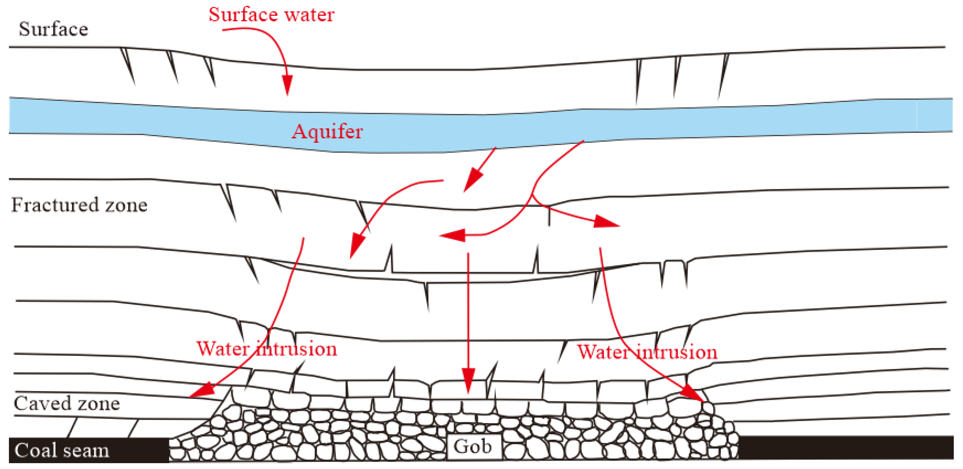
3.1. Engineering background

The No. 8101 working face of the No. 2 coal seam, located in the center of Selian Coal Mine is in the Ordos, Inner Mongolia, China. The ground level corresponding to the mining area is +1382–+1441 m, and the average mining depth of the working face is 170 m. Fully-mechanized mining method is adopted with an average coal thickness of 4.0 m, and the length of working face is 280 m. The strata directly overlying the coal seam mainly consist of the siltstone and sandy mudstone in the Jurassic formation, which were considered as aquitards. Mechanical properties of the 8101 working face’s roof under the gully were tested by the lithology, and the lithology is defined as medium hard.

The surface corresponding to the 8108 working face is undulating and has a gully development with a depth of about 38 m. A short flood will be formed during the rainy season. If the mining crevice penetrates the gully, it will cause surface water to flood into the well, causing the mine to burst. Therefore, it is necessary to study the height of the WCFZ during the mining of the 8101 working face through the gully.

3.2. Model Sample Data

The selection of the sample data is of great significance for the predicting results. There are many factors affecting the height of WCFZ in mining overburden. Based on the previous studies [17,19,36], four major influencing factors affecting the height of WCFZ (H_f ) have been selected: mining depth (H), hard rock proportional coefficient (c), mining thickness (d), length of working face (L). Among them, the hard rock proportional coefficient (c) is the ratio between the accumulated thickness of hard rock strata within the range of the estimated height of WCFZ ($\sum h$) and the estimated height of WCFZ in mining overburden (H_p). The calculation formulas of c and H_p are shown in Equation (8) and Equation (9) respectively.

$$c=\frac{\sum h}{H_p}$$

(8)

$$H_p=(15~20)d$$

(9)

where the H_p can be valued 15–20 times of mining thickness (d) according to local conditions.

On the other hand, the sample data’s gradient distribution for each attribute is directly related to the prediction performance of the model. The wider the gradient distribution, the stronger the representativeness of the established model and the stronger the applicability of the prediction. Based on the above considerations and the characteristics of SVR for processing small sample data, 69 sets of sample data [18,24] were searched to verify the effect of the MPGA-SVR model, as shown in

Table 1. The samples for model training.

No.	H/m	c	d/m	L/m	Hf/m	No.	H/m	c	d/m	L/m	Hf/m
1	412.40	0.09	2.20	157.00	35.40	36	476.40	0.63	3.65	132.00	57.49
2	489.00	0.47	4.50	160.00	54.79	37	515.70	0.35	4.50	147.00	55.00
3	86.10	0.50	4.60	170.00	53.90	38	450.00	0.72	8.00	170.00	86.80
4	472.50	0.53	4.50	132.00	57.45	39	283.90	0.63	5.70	177.90	51.40
5	336.40	0.12	2.00	76.00	27.25	40	499.90	0.47	4.80	150.00	54.79
6	89.00	0.95	2.03	69.00	45.86	41	49.00	0.52	4.00	135.00	45.00
7	424.42	0.26	3.40	120.00	45.10	42	420.06	0.14	3.00	145.00	30.29
8	590.00	0.51	9.00	220.00	76.37	43	516.00	0.74	2.95	206.10	54.50
9	290.00	1.00	2.60	168.00	46.22	44	264.50	0.26	2.80	148.50	40.35
10	290.00	0.18	2.60	168.00	39.14	45	367.00	0.41	7.52	190.00	61.77
11	420.50	0.52	3.00	209.00	52.01	46	434.40	0.46	3.40	136.00	45.10
12	357.00	0.38	7.53	170.00	61.90	47	445.40	0.07	4.00	195.00	38.81
13	649.10	0.23	3.00	186.00	42.99	48	304.00	0.12	3.10	150.00	40.00
14	475.20	0.28	3.90	209.00	49.05	49	362.80	0.33	2.00	138.00	31.62
15	568.60	0.65	3.65	132.00	60.14	50	270.00	0.65	3.80	168.00	54.60
16	557.25	0.45	5.80	186.00	65.25	51	331.00	0.55	7.40	160.00	64.25
17	320.00	0.81	5.00	122.00	67.70	52	499.92	0.47	4.80	150.00	54.00
18	412.55	0.08	2.20	157.00	35.20	53	351.30	0.53	2.00	105.00	36.99
19	312.00	0.24	5.30	145.70	44.20	54	419.03	0.16	3.00	145.00	32.83
20	679.00	0.46	2.10	180.00	44.54	55	357.70	0.33	2.00	128.00	33.96
21	367.00	0.47	7.50	173.50	75.50	56	550.00	0.81	2.40	180.00	55.32
22	403.20	0.10	1.80	120.00	22.61	57	265.00	0.56	2.70	192.00	42.81
23	125.00	0.06	3.00	150.00	22.00	58	320.80	0.16	2.00	128.00	33.01
24	665.00	0.19	7.50	222.00	53.70	59	316.80	0.14	2.00	128.00	31.61
25	433.00	0.52	7.00	168.00	70.30	60	420.00	0.71	3.70	70.00	56.80
26	434.10	0.35	3.00	145.00	47.55	61	478.30	0.54	3.85	209.00	52.15
27	290.00	0.37	2.60	168.00	38.41	62	568.40	0.85	2.94	180.40	57.00
28	485.00	0.36	4.80	175.00	62.50	63	295.00	0.64	2.60	185.00	40.50
29	265.00	0.60	2.60	147.00	43.43	64	453.60	0.16	4.00	195.00	44.96
30	269.00	0.68	2.80	156.00	50.34	65	412.50	0.24	2.20	136.00	35.20
31	387.50	0.55	4.50	175.00	58.50	66	320.00	0.60	1.23	90.00	31.98
32	441.97	0.36	3.40	120.00	48.90	67	411.70	0.30	2.20	136.00	35.21
33	437.17	0.05	3.40	120.00	28.63	68	264.50	0.93	2.80	156.00	44.34
34	463.00	0.62	7.60	116.00	86.40	69	475.00	0.37	6.10	170.00	64.60
35	403.10	0.08	2.00	136.00	22.61

.

The dimension and magnitude of each attribute are different, therefore it is necessary to normalize the sample data, as shown in Equation (10):

$$\{\begin{array}{l}{X}_{ij}=\frac{x_i{}_j-\min (x_i{}_j)}{\max (x_i{}_j)-\min (x_i{}_j)}\\ Y_j=\frac{y_j-\min (y_j)}{\max (y_j)-\min (y_j)}\end{array}$$

(10)

where X_ij is the j-th input sample value in the i-th attribute after normalization, x_ij is the j-th input sample value in the i-th attribute. Y_j is the j-th output sample value after normalization, y_j is the j-th output sample value.

4. Result and Discussion

To test the performance of the MPGA-SVR model, 48 sets of sample data (70%) are selected randomly as training samples, and the other 21 sets of sample data (30%) is selected as test samples. During the development of the SVR model, the MPGA was employed to search for the SVR parameter. The prediction performance of the model was evaluated from two aspects of accuracy and stability. Finally, the total of 69 sets of data were employed to predicting the WCFZ’s height of 8101 working face. All computational works in this model were implemented in MATLAB 2017b programming environment based on the CPU of Xeon(R) E3-1230 3.30GHz processor.

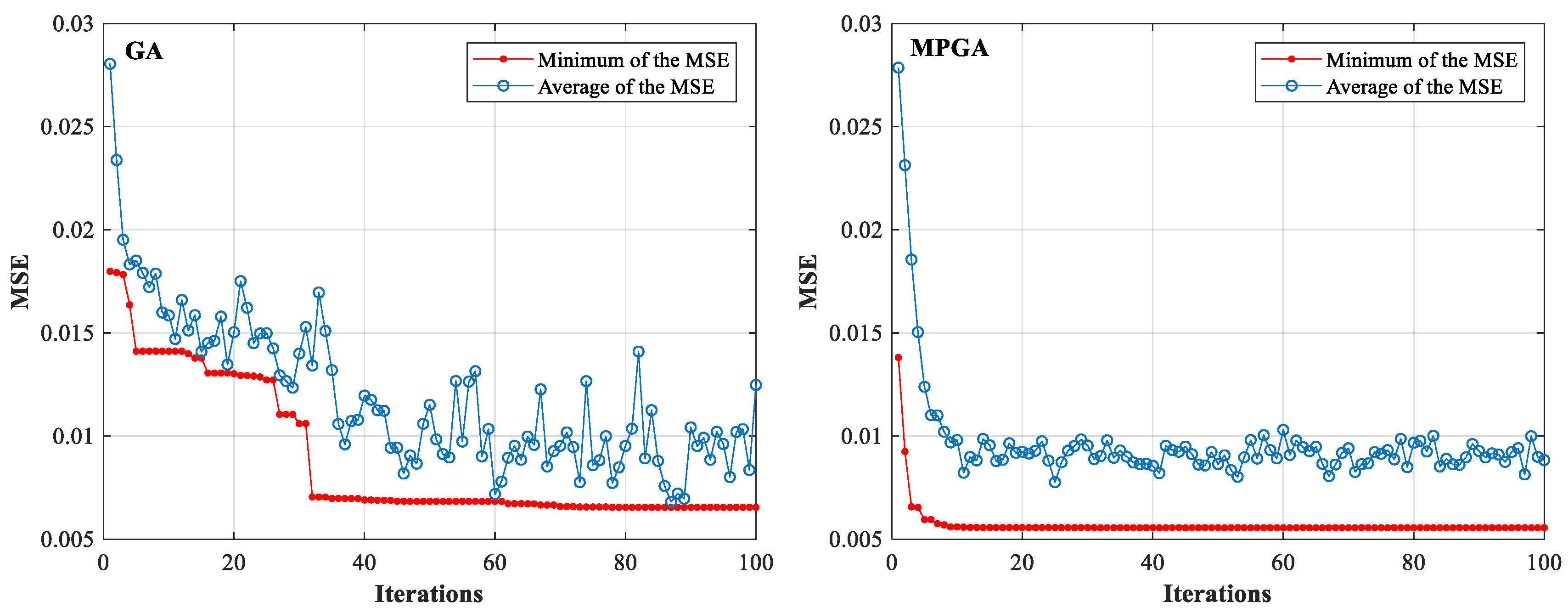
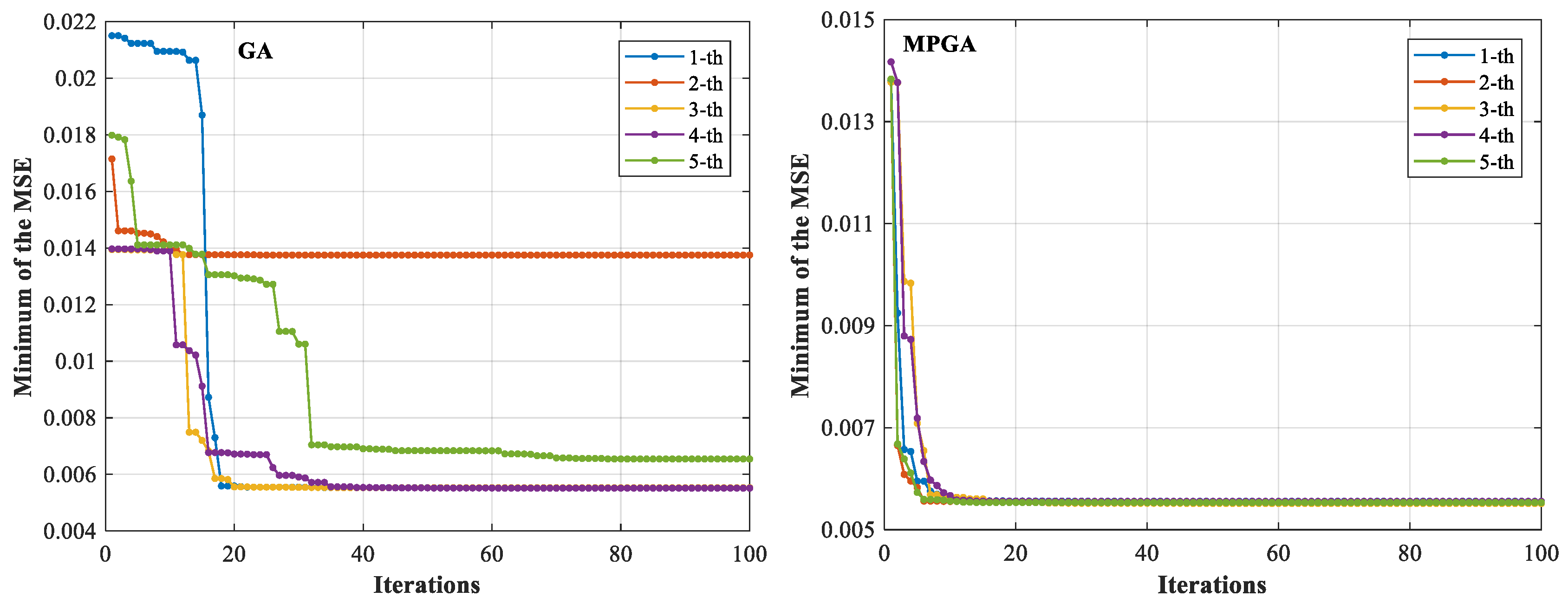
4.1. The Parametric Optimization Process of the SVR Model

After 100 generations of evolution, the target parameters were obtained based on the randomly selected 48 sets of training sample data. The parametric optimization process of GA and MPGA are shown in Figure 3.

In order to reflect the performance advantages of MPGA, both of the GA and MPGA were adopted to search for the parameters respectively. Each algorithm’s performance was assessed by the mean squared error (MSE) between the standardized predicted results ($H_{sf}^{\prime }$) and actual results (H_sf), and it was expressed as Equation (11):

$$MSE=\frac{1}{n}{\displaystyle \sum _{j=1}^n{(H_{sf}-H_{sf}^{\prime })}^2}$$

(11)

In the process of parameters optimization, the GA tends to converge after 32 generations of evolution, and the value of MSE is reduced from 0.018 to 0.007. The MPGA converges after only seven generations of evolution, and the value of MSE is reduced from 0.014 to 0.005. On the other hand, the average of the MSE in GA has a larger range of change than MPGA. Therefore, the MPGA has higher search accuracy, and significantly improves the slow convergence of GA. Finally, the optimal fitness parameter values selected are shown in

Table 2. Optimal parameters obtained according to GA and MPGA.

Model	Parameter	Optimal Value
GA	C	19.30
	g	0.10
MPGA	C	2.58
	g	0.36

.

To further verify the stability of the algorithms during the parameters search process, five times of repeated searches were performed, as shown in Figure 4. Comparing with the result we can see that the GA has a large MSE of 0.014 in the parameter optimization process of the second time, which is caused by the premature convergence. For the result of the MPGA, the MSE error results of five iterations were basically consistent with an average value of 0.0055.

Therefore, MPGA has higher accuracy and stability in the process of parameter optimization for SVR.

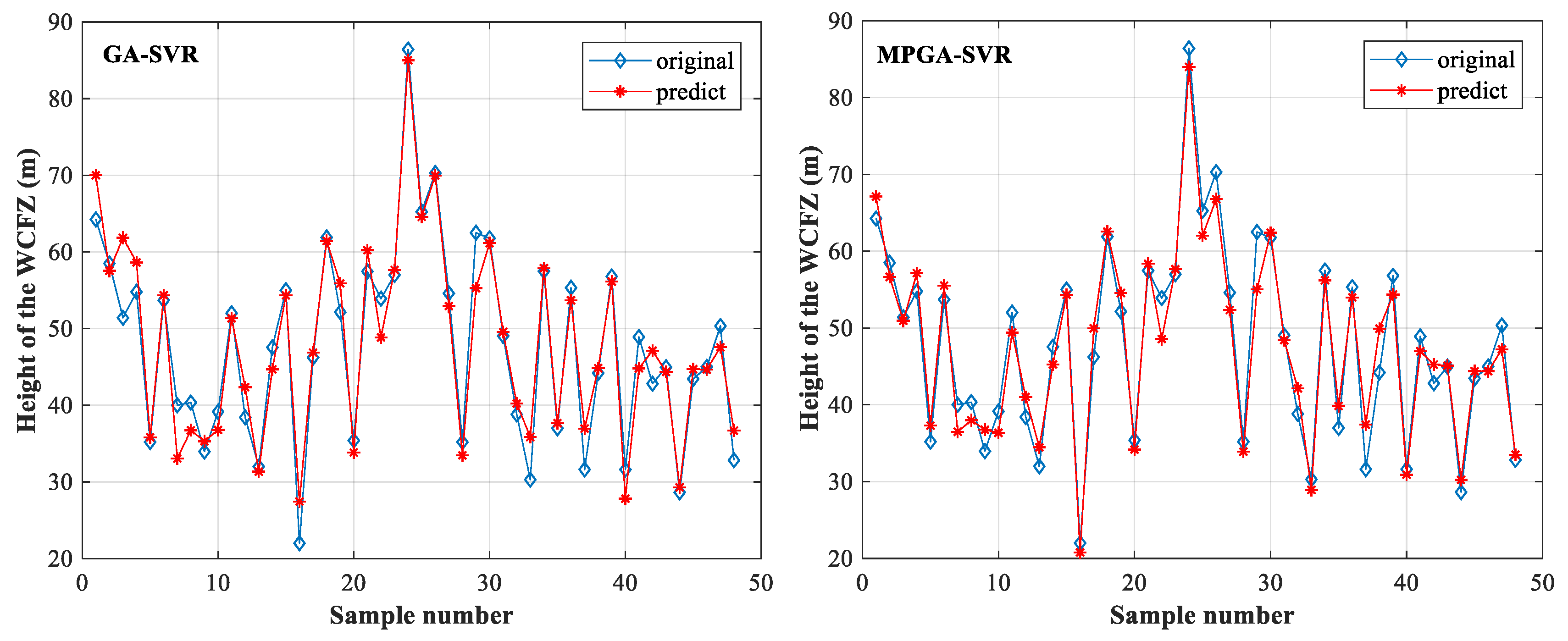
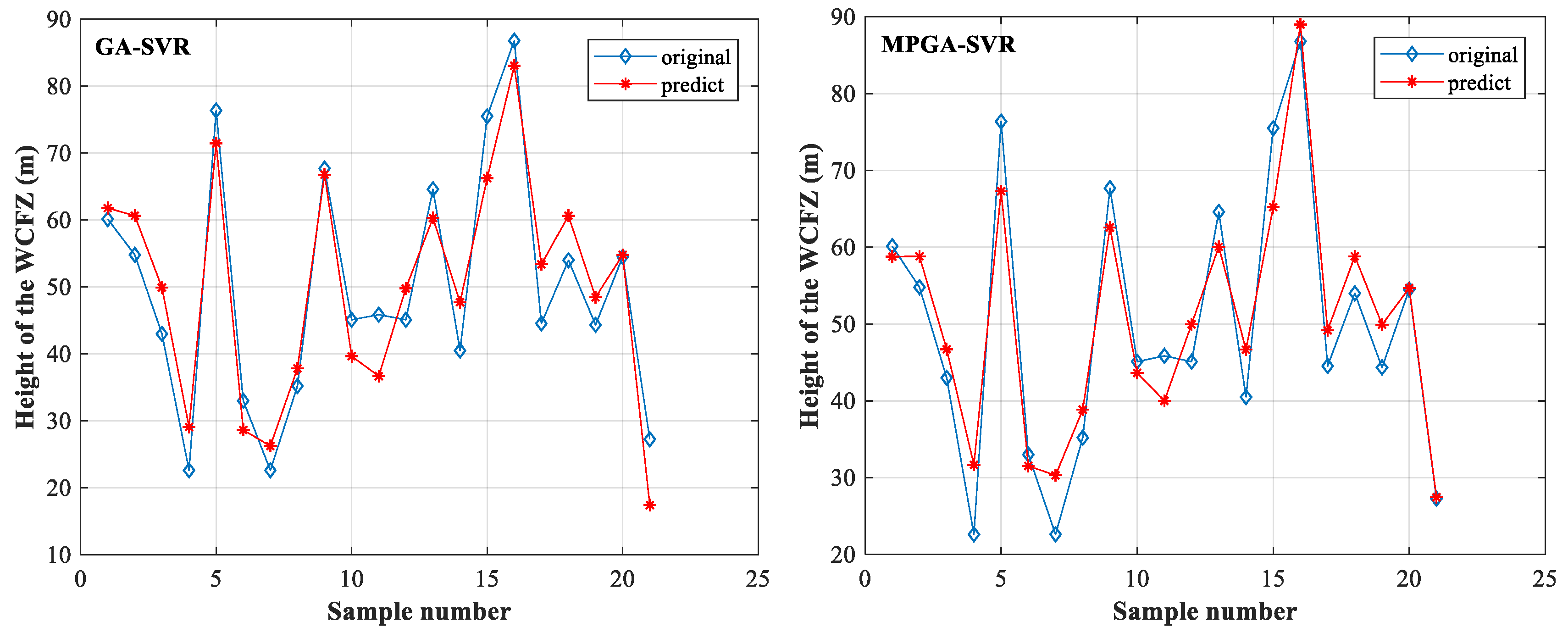
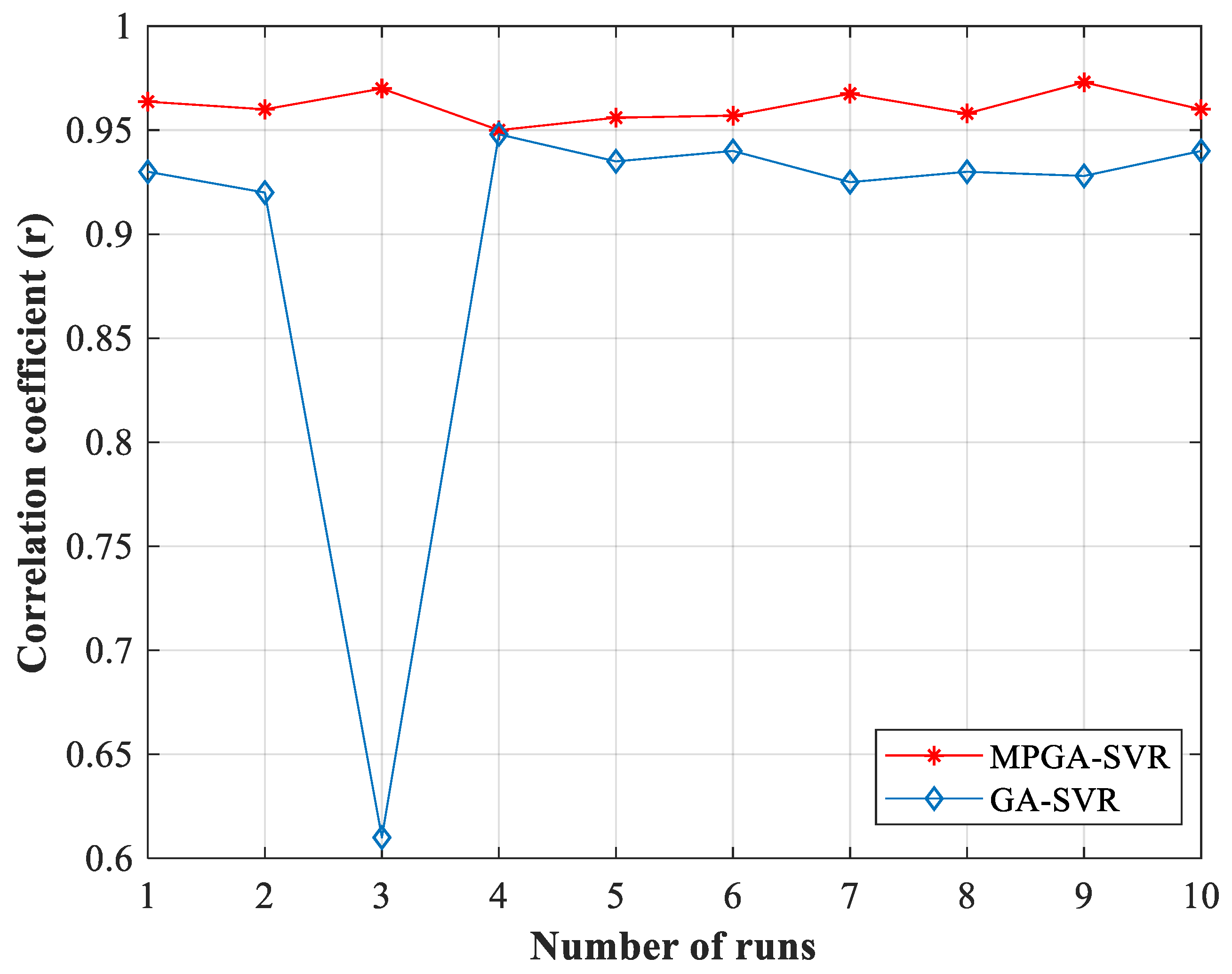
4.2. The Test of the MPGA-SVR Model

In order to accurately and objectively map the performance of MPGA-SVR model, the correlation coefficient (r) between the predicted results ($H_f^{\prime }$) and experimental results (H_f) were used:

$$r(H_f,H_f^{\prime })=\frac{Cov(H_f,H_f^{\prime })}{\sqrt{Var[H_f]Var[H_f^{\prime }]}}$$

(12)

where $Cov(H_f,H_f^{\prime })$ is the covariance between H_f and $H_f^{\prime }$, Var[H_f] is the variance of H_f and Var[$H_f^{\prime }$] is the variance of $H_f^{\prime }$.

The parameters obtained from the GA and MPGA model were employed respectively to predict the training samples and test samples, and the results were shown in Figure 5 and Figure 6. Based on the Equations (11) and (12), the r and MSE of the two models were calculated as

Table 3. Optimal parameters obtained after GA and MPGA search.

Sample data	Prediction Model	MSE (m2)	Correlation Coefficient (r)
Training sample	GA-SVR	11.13	0.96
	MPGA-SVR	7.29	0.97
Test sample	GA-SVR	34.91	0.93
	MPGA-SVR	28.70	0.96

.

Comparing with the results we can see that the MPGA-SVR model has the lower MSE and higher r for both of the training sample and test sample. Therefore, the MPGA-SVR model has a better performance on accuracy compared with the GA-SVM.

In addition to accuracy, stability is also an important index to test the predictive performance of the model. In this paper, 10 repeated trainings and predictions were performed through the two models respectively for the same grouped data, and the prediction results were shown in Figure 7. As it can be seen from Figure 7, the GA-SVR model has a poor prediction effect in the third time with a value of 0.6. However, the correlation coefficient of the MPGA-SVR model is higher than 0.95 every time.

Therefore, the MPGA-SVR has a better prediction performance from the results of training sample and test sample.

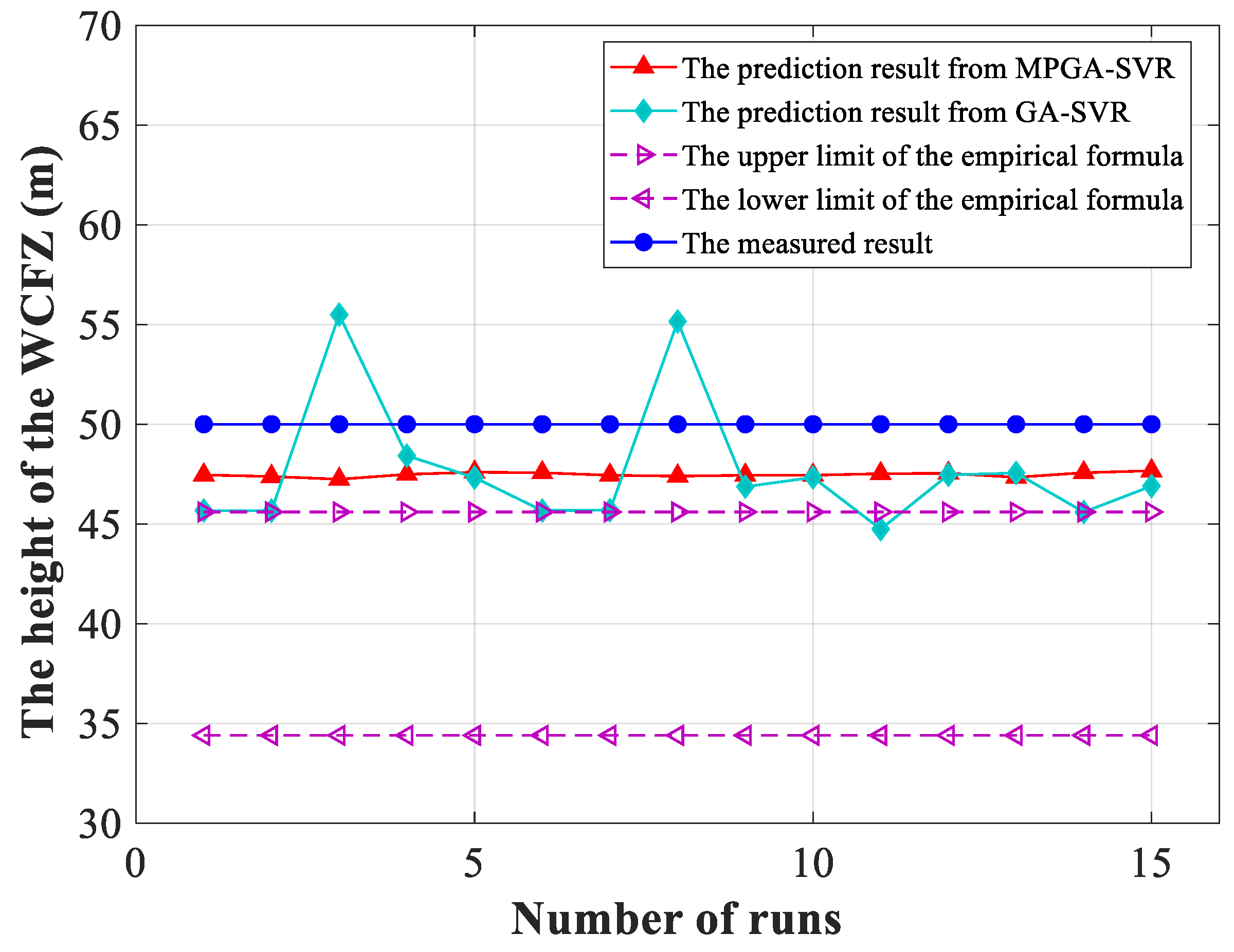
4.3. Application of the MPGA-SVR Model

In order to further verify the validity of the MPGA-SVR model for the prediction of water-crushing zone and its engineering application value, the prediction of the WCFZ’s height for the 8101 working face is carried out.

In this section, 69 sets of data were used as training samples to predict the height of the WCFZ during the mining of the 8101 working face through the gully. For comparison with traditional methods, the empirical formula method, GA-SVR and MPGA-SVR model were applied, respectively.

The traditional empirical formula was proposed by Liu Tianquan in the early 1980s based on regression statistical analysis of data from mid-eastern China’s Carboniferous Permian coalfield. Mechanical properties of the 8101 working face’s roof under the gully were tested by the lithology, and the lithology is defined as medium hard. Therefore, the predicted height of the WCFZ according to the empirical formula method (listed in

Table 4. Experiential computing formula of WCFZ height.

Lithology	Computing Formula
Hard	$H_f^{\prime }=\frac{100\sum M}{1.2\sum M+2.0}\pm 8.9$
Medium hard	$H_f^{\prime }=\frac{100\sum M}{1.6\sum M+3.6}\pm 5.6$
Weak	$H_f^{\prime }=\frac{100\sum M}{3.1\sum M+5.0}\pm 4.0$
Extremely weak	$H_f^{\prime }=\frac{100\sum M}{5.0\sum M+8.0}\pm 3.0$

) is:

$$H_f^{\prime }=\frac{100\sum M}{1.6\sum M+3.6}\pm 5.6=40\pm 5.6(\mathrm{m})$$

(13)

where the $\sum M$ is the cumulative thickness of mining coal seam, and the value is equal to the coal thickness (d) of 4 m here.

In this case, the estimated height (H_p) of the WCFZ is 20 times of the coal thickness (d), and the cumulative thickness ($\sum h$) of the hard rock above the coal roof is 73.72 m. The hard rock proportional coefficient (c) is 0.9215 according to the Equation (8).

In order to compare the accuracy and stability of the GA-SVR and MPGA-SVR models at the same time, the prediction results were obtained by repeated calculation 15 times, the prediction height of the WCFZ is shown in Figure 8.

After the actual measurement on site, the height of the WCFZ is approximately 50 m. Aiming to show the error of different prediction results, the absolute relative error φ between the prediction result and measured result was adopted, which is defined as Equation (14). The result was shown in Figure 9.

$$\phi =\frac{\left|H_f-H_f^{\prime }\right|}{H_f}$$

(14)

From the Figure 8 and Figure 9, we can see that the empirical formula’s prediction height of the WCFZ is from 34.4 m to 45.6 m, and the absolute relative error is from 0.088 to 0.312. As the empirical formula method considers a single influencing factor only, so the error is the largest. Although the average prediction height of the WCFZ by the GA-SVR and MPGA-SVR models are both about 47.5 m, but the GA-SVR model’s prediction result varies greatly each time with a biggest error of 0.11. That is because the GA has premature convergence when the individuals in the population tend to be in the same state prematurely and stop evolution. It is obvious that a consistent result can always be obtained for each calculation by the MPGA-SVR model with an absolute relative error of 0.005, while the result obtained by the GA has greater uncertainty. Based on the comprehensive consideration of various factors that affect the development of the water-conducting fracture zone, the MPGA was used to select more appropriate model parameters for the SVR prediction model. Hence, the MPGA-SVR model exhibits a better accuracy and stability performance comparing with the other methods in this case. In addition, the model will be continuously enriched and updated in practice to make it more accurate and generalizable.

5. Conclusions

In this paper, the MPGA-SVR model is proposed as a novel approach to predict the height of the WCFZ. The prediction accuracy and stability of the WCFZ’s height have been greatly improved by the MPGA-SVR model with the parameters of mining depth, hard rock proportional coefficient, mining thickness, length of working face.

In the process of parameter optimization, the MPGA properly resolves the premature convergence and slow convergence of GA by co-evolving multiple populations with different genetic parameters, and the local and global search ability of the model is further improved. Finally, a more suitable parameter is obtained to predict the height of WCFZ prediction, and the prediction results have a high correlation coefficient, low mean square errors and good stability, which is very close to the experimental result. Comparing with the traditional method, since the model of MPGA-SVR considers many influencing factors at the same time, unlike the traditional empirical formula, only the unilateral factors are considered. Therefore, the model proposed in this paper provides a more reasonable solution to obtain the height of the WCFZ, which is of great significance for the safe and efficient mining of coal mines. Based on the algorithm proposed in this paper, we can further study and design different migration mechanisms and several sub-population hierarchical execution architectures of GA in multi-population mechanisms to obtain more accurate results.

References

1. Chang, S.; Zhuo, J.; Meng, S.; Qin, S.; Yao, Q. Clean coal technologies in China: Current status and future perspectives. Engineering 2016, 2, 447–459. [Google Scholar] [CrossRef]
2. Liu, S.L.; Li, W.P.; Wang, Q.Q. Height of the Water-Flowing Fractured Zone of the Jurassic Coal Seam in Northwestern China. Mine Water Environ. 2018, 37, 312–321. [Google Scholar] [CrossRef]
3. Liu, Y.; Liu, Q.M.; Li, W.P.; Li, T.; He, J.H. Height of water-conducting fractured zone in coal mining in the soil-rock composite structure overburdens. Environ. Earth Sci. 2019, 78. [Google Scholar] [CrossRef]
4. Feng, X.; Zhang, N.; Chen, X.; Gong, L.; Lv, C.; Guo, Y. Exploitation contradictions concerning multi-energy resources among coal, gas, oil, and uranium: A case study in the Ordos Basin (Western North China Craton and Southern Side of Yinshan Mountains). Energies 2016, 9, 119. [Google Scholar] [CrossRef] [Green Version]
5. Wu, Q.; Liu, Y.; Zhou, W.; Wu, X.; Liu, S.; Sun, W.; Zeng, Y. Assessment of water inrush vulnerability from overlying aquifer using GIS-AHP-based ’three maps-two predictions’ method: A case study in Hulusu coal mine, China. Q. J. Eng. Geol. Hydrogeol. 2015, 48, 234–243. [Google Scholar] [CrossRef]
6. Adhikary, D.P.; Guo, H. Measurement of longwall mining induced strata permeability. Geotech. Geol. Eng. 2014, 32, 617–626. [Google Scholar] [CrossRef]
7. Han, Y.; Cheng, J.; Huang, Q.; Zou, D.H.; Zhou, J.; Huang, S.; Long, Y. Prediction of the height of overburden fractured zone in deep coal mining: Case study. Arch. Min. Sci. 2018, 63, 617–631. [Google Scholar] [CrossRef]
8. Zhang, Y.; Cao, S.; Gao, R.; Guo, S.; Lan, L. Prediction of the Heights of the Water-Conducting Fracture Zone in the Overlying Strata of Shortwall Block Mining Beneath Aquifers in Western China. Sustainability 2018, 10, 1636. [Google Scholar] [CrossRef] [Green Version]
9. Wei, J.; Wu, F.; Yin, H.; Guo, J.; Xie, D.; Xiao, L. Formation and height of the interconnected fractures zone after extraction of thick coal seams with weak overburden in western China. Mine Water Environ. 2017, 36, 59–66. [Google Scholar] [CrossRef]
10. Zhang, D.; Li, W.; Lai, X.; Fan, G.; Liu, W. Development on basic theory of water protection during coal mining in northwest of China. J. China Coal Soc. 2017, 42, 36–43. [Google Scholar]
11. Lawson, H.E.; Tesarik, D.; Larson, M.K.; Abraham, H. Effects of overburden characteristics on dynamic failure in underground coal mining. Int. J. Min. Sci. Technol. 2017, 27, 121–129. [Google Scholar] [CrossRef]
12. Liu, X.; Tan, Y.; Ning, J.; Tian, C.; Wang, J. The height of water-conducting fractured zones in longwall mining of shallow coal seams. Geotech. Geol Eng. 2015, 33, 693–700. [Google Scholar] [CrossRef]
13. Zhang, Y.; Tu, S.; Bai, Q.; Li, J. Overburden fracture evolution laws and water-controlling technologies in mining very thick coal seam under water-rich roof. Int. J. Min. Sci. Technol. 2013, 23, 693–700. [Google Scholar] [CrossRef]
14. Pillar Design and Mining Regulations Under Buildings, Water, Rails and Major Roadways; China Coal Industry Publishing House: Beijing China, 2000.
15. Yang, G.; Chen, C.; Gao, S.; Feng, B. Study on the height of water flowing fractured zone based on analytic hierarchy process and fuzzy clustering analysis method. J. Min. Saf. Eng. 2015, 32, 206–212. [Google Scholar]
16. Zhao, D.; Wu, Q. An approach to predict the height of fractured water-conducting zone of coal roof strata using random forest regression. Sci. Rep. 2018, 8, 1–12. [Google Scholar] [CrossRef] [Green Version]
17. Chai, H.; Zhang, J.; Yang, C. Prediction of water-flowing height in fractured zone of overburden strata based on GA-SVR. J. Min. Saf. Eng. 2018, 35, 359–365. [Google Scholar]
18. Ma, Y.; Wu, Q.; Zhang, Z.; Hong, Y.; Guo, L.; Tian, H.; Zhang, L. Research on prediction of water conducted fissure height in roof of coal mining seam. Coal Sci. Technol. 2008, 5, 59–62. [Google Scholar]
19. Wu, Q.; Shen, J.J.; Liu, W.T.; Wang, Y. A RBFNN-based method for the prediction of the developed height of a water-conductive fractured zone for fully mechanized mining with sublevel caving. Arab. J. Geosci. 2017, 10, 9. [Google Scholar] [CrossRef]
20. Qi, Y.; Zhao, X.; Luo, B.; Luo, M. GA-SVR Prediction of Failure Depth of Coal Seam Floor Based on Small Sample Data. Proceedings of the Fifth National Conference on Computer Mathematics, Hong Kong, China, 2013. Available online: http://www.ipcbee.com/vol52/017-ICGES2013-G30006.pdf (accessed on 28 February 2020).
21. Al-Anazi, A.F.; Gates, I.D. Support vector regression to predict porosity and permeability: Effect of sample size. Comput. Geosci. 2012, 39, 64–76. [Google Scholar] [CrossRef]
22. Dhiman, H.S.; Deb, D.; Guerrero, J.M. Hybrid machine intelligent SVR variants for wind forecasting and ramp events. Renew. Sustain. Energy Rev. 2019, 108, 369–379. [Google Scholar] [CrossRef]
23. Jiang, X.; Lu, W.X.; Hou, Z.Y.; Zhao, H.Q.; Na, J. Ensemble of surrogates-based optimization for identifying an optimal surfactant-enhanced aquifer remediation strategy at heterogeneous DNAPL-contaminated sites. Comput. Geosci. 2015, 84, 37–45. [Google Scholar] [CrossRef]
24. Sun, Y.; Wang, Y.; Deng, X. Analysis the height of water conducted zone of coal seam roof based on GA-SVR. J. China Coal Soc. 2009, 34, 1610–1615. [Google Scholar]
25. Roushangar, K.; Koosheh, A. Evaluation of GA-SVR method for modeling bed load transport in gravel-bed rivers. J. Hydrol. 2015, 527, 1142–1152. [Google Scholar] [CrossRef]
26. Holland, J.H. Adaptation in Natural and Artificial Ssystems; University of Michigan Press: Ann Arbor, MI, USA, 1975. [Google Scholar]
27. Yeh, C.W.; Jang, S.S. The development of information guided evolution algorithm for global optimization. J. Glob. Optim. 2006, 36, 517–535. [Google Scholar] [CrossRef]
28. Vapnik, V.N. The Nature of Statistical Learning Theory, 2nd ed.; Statistics for Engineering and Information Science; Springer: New York, NY, USA, 2000. [Google Scholar]
29. Hou, Z.Y.; Lu, W.X. Comparative study of surrogate models for groundwater contamination source identification at DNAPL-contaminated sites. Hydrogeol. J. 2018, 26, 923–932. [Google Scholar] [CrossRef]
30. Jayasumana, S.; Hartley, R.I.; Salzmann, M.; Li, H.; Harandi, M.T. Kernel Methods on riemannian manifolds with gaussian RBF kernels. IEEE Trans. Pattern Anal. Mach. Intell. 2015, 37, 2464–2477. [Google Scholar] [CrossRef] [Green Version]
31. Du, H.; Chen, W.; Zhu, Q.; Liu, S.; Zhou, J. Identification of weak peaks in X-ray fluorescence spectrum analysis based on the hybrid algorithm combining genetic and Levenberg Marquardt algorithm. Appl. Radiat. Isot. 2018, 141, 149–155. [Google Scholar] [CrossRef]
32. Joo, A.; Ekart, A.; Neirotti, J.P. Genetic Algorithms for Discovery of Matrix Multiplication Methods. IEEE Trans. Evol. Comput. 2012, 16, 749–751. [Google Scholar] [CrossRef] [Green Version]
33. Li, X.; Wang, Z.X.; Chan, F.T.S.; Chung, S.H. A genetic algorithm for optimizing space utilization in aircraft hangar shop. Int. Trans. Oper. Res. 2019, 26, 1655–1675. [Google Scholar] [CrossRef]
34. Mera, N.S.; Elliott, L.; Ingham, D.B. A multi-population genetic algorithm approach for solving ill-posed problems. Comput. Mech. 2004, 33, 254–262. [Google Scholar] [CrossRef]
35. Jiao, Y.L.; Xing, X.C.; Zhang, P.; Xu, L.C.; Liu, X.R. Multi-objective storage location allocation optimization and simulation analysis of automated warehouse based on multi-population genetic algorithm. Concurr. Eng. Res. Appl. 2018, 26, 367–377. [Google Scholar] [CrossRef]
36. Li, Z.; Xu, Y.; Li, L.; Zhai, C. Forecast of the height of water flowing fractured zone based on BP neural networks. J. Min. Saf. Eng. 2015, 123, 39–44. [Google Scholar]
Figure 1. The development of a water-conducting fracture zone (WCFZ) in mining overburden strata after mining.
Sustainability 12 01809 g001
Figure 2. Flowchart showing the implementation procedure of multi-population genetic algorithm (MPGA) for searching support vector regression (SVR) optimal parameters.
Sustainability 12 01809 g002
Figure 3. The parametric optimization process of GA and MPGA.
Sustainability 12 01809 g003
Figure 4. The repetitive parametric optimization process of GA and MPGA for five times.
Sustainability 12 01809 g004
Figure 5. The comparisons of prediction results of training samples.
Sustainability 12 01809 g005
Figure 6. The comparisons of prediction results of test samples.
Sustainability 12 01809 g006
Figure 7. The comparisons of prediction results for 10 times repeatedly.
Sustainability 12 01809 g007
Figure 8. The prediction height of the WCFZ for different methods.
Sustainability 12 01809 g008
Figure 9. The absolute relative error of the prediction results for different methods.
Sustainability 12 01809 g009