Article

Landscape Management through Change Processes Monitoring in Iran

by
Mohsen Zabihi
1,2,*,
Hamidreza Moradi
1,
Mehdi Gholamalifard
3,
Abdulvahed Khaledi Darvishan
1 and
Christine Fürst
2,*
1
Department of Watershed Management Engineering, Faculty of Natural Resources, Tarbiat Modares University, Noor 46417-76489, Iran
2
Department of Sustainable Landscape Development, Institute for Geosciences and Geography, Martin Luther University Halle-Wittenberg, 06120 Halle, Germany
3
Department of the Environment Sciences, Faculty of Natural Resources, Tarbiat Modares University, Noor 46417-76489, Iran
*
Authors to whom correspondence should be addressed.
Sustainability 2020, 12(5), 1753; https://doi.org/10.3390/su12051753
Submission received: 3 February 2020 / Revised: 22 February 2020 / Accepted: 24 February 2020 / Published: 26 February 2020
(This article belongs to the Special Issue Landscape Ecology for Sustainability)

Abstract

:
The presented research investigated and predicted landscape change processes (LCPs) in the Talar watershed, northern Iran. The Land Change Modeler was used for change analysis, transition potential modeling, and prediction of land use/land cover (LULC) map. The evaluation of projected LULC map was performed by comparing the real and predicted LULC maps for the reference year, 2014. Landscape metrics and change processes were investigated for the period 1989–2014 and for exploring the situation in 2030. Results illustrated that the increase in agricultural land and residential areas took place at the expense of forest and rangeland. The distance from forests was the most sensitive parameter for modeling the transition potentials. The modelling of the LULC change projected the number of patches, the landscape shape index, interspersion and juxtaposition index, and edge density, Euclidean nearest-neighbor distance, and area-weighted shape index will amount to 65.3, 7.63, 20.1, 8.77, −1.35, and 0.61% as compared to 2014, respectively. Our findings indicated that the type of change processes that occurred was not entirely the same in 1989–2000 and 2000–2014. In addition, change processes in the creation of dry farming, orchard, and residential classes, attrition of forest and rangeland categories, and dissection in irrigated farming are projected. The dynamics of landscape metrics and change processes combined in one analytical framework can facilitate understanding and detection of the relationship between ecological processes and landscape pattern. The finding of current research will provide a roadmap for improved LULC management and planning in the Talar watershed, southern coast of the Caspian Sea.

Graphical Abstract

1. Introduction

Quantifying the relationship between different landscape criteria including metrics and change processes is challenging [1], but the investigation and management of landscape change and division that is listed as a threat for sustainable development of the environment [2] is of global relevance to achieve the UN Sustainable Development Goals (SDGs). Reasons, processes, and impacts of landscape change have been an arguable issue in past decades [3]. Accordingly, understanding change processes of landscape and influencing factors, namely biophysical and anthropogenic, has become a priority for researchers, managers, and decision makers [4,5,6,7]. In this regard, population growth as an anthropogenic factor is the main reason for land use/land cover (LULC) and landscape change on a global scale [8,9,10].
Land use/land cover change (LULCC) is addressed as the most environmental policy issue in the future, which landscape ecology can help to solve the related problems [11]. The change of socioeconomic situation is one of the influencing factors on ecological processes of the landscapes [12]. In this regard, landscape metrics (LMs) and the types of landscape change processes (LCPs) are two relevant approaches to interpret the drivers and character of landscape changes. LMs are utilized for measuring and quantifying the spatial pattern (composition, configuration, and connectivity) of landscapes at a certain time [13,14], while LCPs compare times series LULC maps to detect the changes. In addition, change processes including aggregation, attrition, creation, dissection, among others, measure the nature of the change within each LULC class over time. From the landscape ecology perspective, configuration and composition have an important role in the determination and description of natural habitats, hydrological processes, energy, and the nutrient cycle [15]. Therefore, these two approaches can be implemented for interaction analysis of anthropogenic and biophysical factors in social-ecological systems [16,17]. Simplifying the interaction between human and ecosystems using LCPs is one of the most important applications to operationalize them for policy recommendations. The analysis of LCPs is hypothesized as a holistic and integrated approach because it includes landscape metrics as well. Moreover, a large number of LMs may establish ambiguities and confusion for correct decision and policy-making. In contrast, measuring the changes within each LULC category by LCPs provides concrete recommendations for land management [18]. Therefore, analysis and deliberation of LCPs and their effects on biogeophysical factors is more comprehensive than LMs for suitable decision-making.
Landscape represents the effect of anthropogenic (social, economic, political) and biophysical factors on different ecosystems. Existing interaction between manifold factors, particularly population growth, socioeconomic needs, and political changes had a negative impact on the ecosystems in the Talar watershed, which is a representative watershed of northern Iran. Destructive floods [19], different types of soil erosion, landslides, soil and water resources pollution, deforestation, residential area development, and road construction are negative consequences in the studied watershed. A landscape-based sequential analysis of change processes in different ecosystems (LULC categories) is needed to account for critical development trends. Although intensive research on the interrelations between LULC and LMs [20,21,22] has been conducted, research about temporal changes in LCPs, LMs, and LULC has not yet been brought together. Hence, the use of LCPs is a step forward in connecting landscape ecology with sustainable landscape development and planning. The presented paper introduces a landscape framework for planning and detecting anthropogenic effects in the Talar watershed using LCPs. It introduces the impacts from human interventions at different spatiotemporal scales by investigating LMs and LCPs. So, the objective of the present research is the monitoring (1989–2014) and prediction (2030) of landscape metrics and change processes using Landsat satellite images over 25 years in the Talar watershed, northern Iran.

2. Materials and Methods

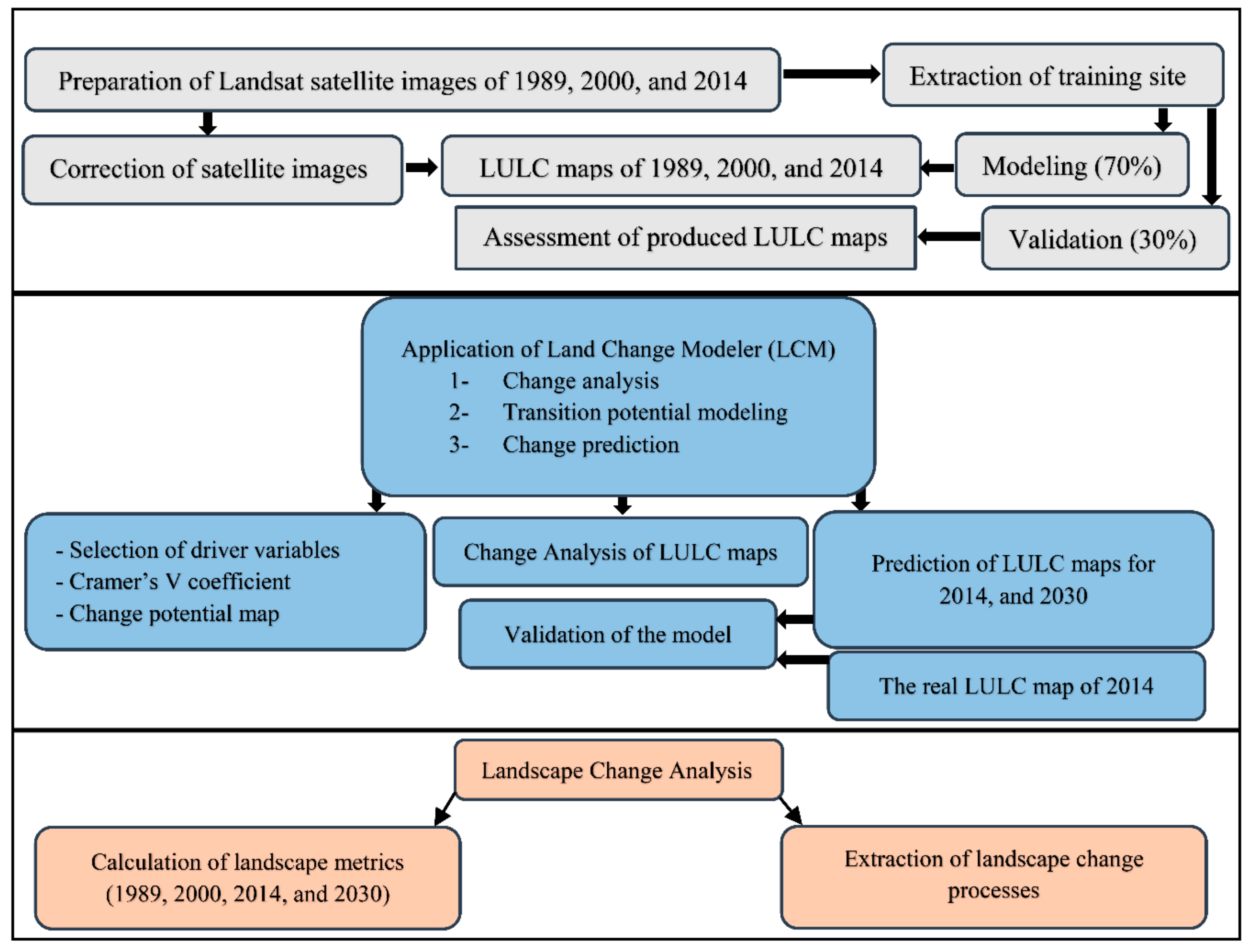
2.1. Overview of Study Methodology
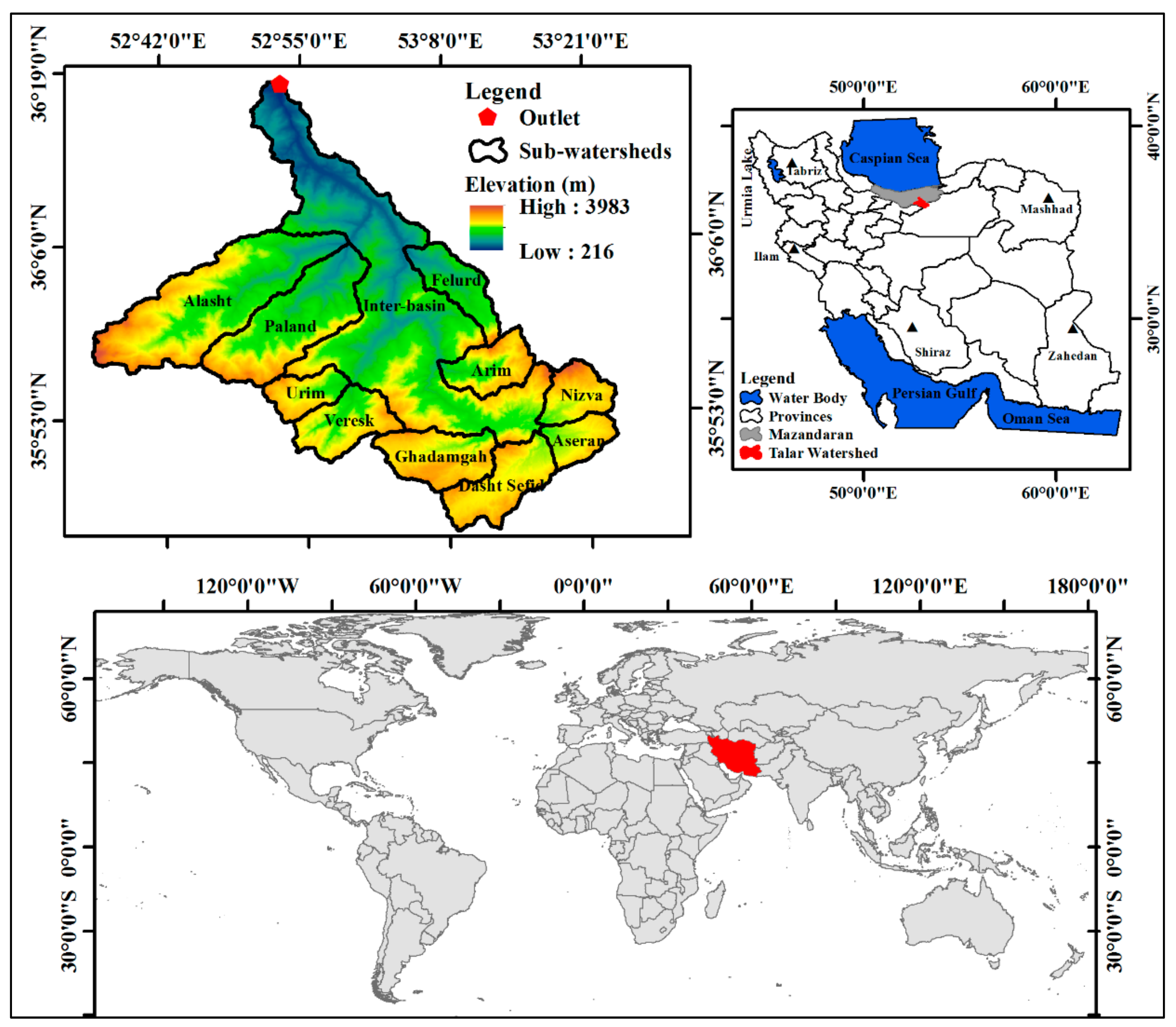
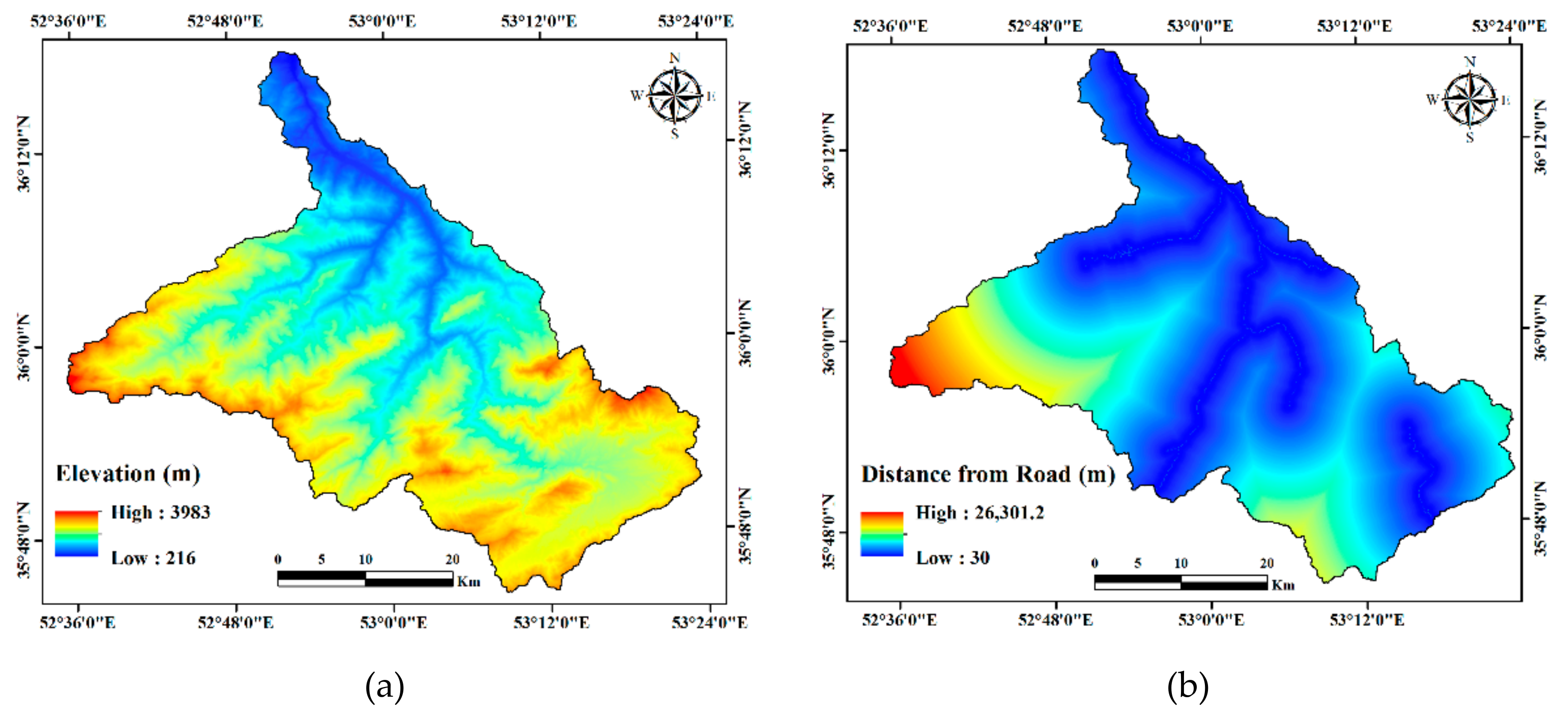
Our research is structured into three main steps (see Figure 1). First, LULC changes of the Talar watershed are investigated using satellite images from 1989 to 2014. Second, the LULC map for 2030 is modelled using Multi-Layer Perceptron (MLP) and Markov chain procedures. Finally, LMs and LCPs are investigated for the time period of 1989–2030 to characterize the landscape changes.

2.2. Study Area

The present research was implemented in the Talar watershed, southern Caspian Sea, Iran. The study area in the Mazandaran, Semnan, and Tehran Provinces of Iran lies between 52.59˚ and 53.39˚ longitude, and 35.73˚and 36.31˚ latitude. The area’s elevation ranges from 216 to 3983 meters above sea level. The average annual rainfall (Mediterranean climate) is approximately 552.7 mm, and annual minimum and maximum temperatures are 7.7 and 21.1 ˚C, respectively. The Talar River, with an average annual discharge of 7.95 m3s−1, drains out about 1764 km2 of the study area and finally reaches the Caspian Sea [23]. Sedimentary, igneous, and continental rocks are the most important bedrocks in the research area. The majority of the bedrock’s origin is from the Mesozoic Era. Shirgah, Pol Sefid, Zirab, Veresk, and Alasht are the main residential areas located in the Talar watershed. Fertile agricultural lands and a high amount of precipitation, along with a temperate climate condition, have increased the change pressures on the original Hyrcanian forests (7% of Iran’s area), which stretches 850 km along the southern coast of the Caspian Sea and northern slope of the Alborz Mountains and have been listed as world heritage of UNESCO. Urban sprawl, deforestation, and agricultural expansion are thus the most dominant LULC changes in northern Iran [9], especially in the Talar watershed. Also, 3234 species of vascular plants, 180 species of birds, and 58 mammal species in the mentioned forests [24,25] place it as a special ecological reserve in the world, with outstanding value for nature conservation. Figure 2 indicates the geographical location of the Talar watershed in the world and Iran.

2.3. LULC Mapping and Detection

Landsat satellite images were applied for the preparation of LULC maps in the Talar watershed. Three Landsat images of the TM (from the years 1989 and 2000) and OLI (from the year 2014) sensors were downloaded from the United States Geological Survey (USGS) website (www.earthexplorer.usgs.gov). An atmospheric correction of mentioned images was performed using the dark-object subtraction procedure [24,26]. Subsequently, training samples for each LULC class were extracted from extensive field surveys, False Color Composite (FCC) of satellite images, and Google Earth in the three reference years. The extracted training samples were divided randomly to 70% and 30% datasets, which were utilized for modeling and validation of LULC maps, respectively. Subsequently, a Support Vector Machine (SVM) algorithm was implemented for LULC mapping in the reference years [27]. Finally, Kappa coefficient and overall accuracy were computed and employed to assess the LULC maps through a comparison of produced LULC maps and real ground data [24,27,28,29]. ENVI 5.3 and ArcGIS 10.5 were used to implement LULC change mapping and detection.

2.4. LULC Change Analysis

The change analysis of the LULC maps was performed by Land Change Modeler (LCM) in TerrSet 18.31 [30]. To investigate the changes, comparisons of the LULC maps of 1989 with 2000, 2000 with 2014, and 1989 with 2014 were implemented. In addition, gains, losses, and net changes for each LULC category were analyzed and checked.

2.5. LULC Transition Potential Modeling

The types of LULC changes to modeling of transition potentials were selected based on the observed LULC changes in the Talar watershed. Several explanatory variables were selected according to literature review [24,31] and data accessibility and were tested based on Cramer’s V coefficient. This coefficient displays the potential explanatory power of a variable for LULC change. If the value of Cramer’s V coefficient is higher than 0.15, the variable is acceptable and can be used for LULC change modeling [8,32]. Elevation, distance from roads, distance from rivers, distance from dry farming, distance from forests, distance from rangelands, distance from residential areas, and evidence likelihood to change were examined. The digital elevation model was acquired from National Cartographic Center (NCC) of Iran. All distances were extracted from earlier LULC maps for the investigated periods of 1989–2000 and 2000–2014 using Euclidean distance algorithms in ArcGIS 10.5. Evidence for the likelihood of change was prepared in a variable transformation utility panel of LCM in TerrSet. Evidence likelihood transformation is a very effective means of incorporating categorical variables into the analysis [30]. Modeling of the transition potential was executed by using MLP and Back-propagation algorithm [33,34]. MLP, which is based on a neural network, models the nonlinear and complex relationship among variables without considering the form of data distribution. Additionally, MLP investigates and conducts the sensitivity analysis of explanatory factors. For this attempt, each independent variable was forced to be constant, and then the accuracy of the model was measured.

2.6. LULC Change Prediction

Produced transition potential maps were applied for the prediction of quantitative changes. The amount of changes in each transition period, and change allocation to each LULC class were explored using the Markov chain method [35,36]. To predict the LULC map of 2014, LULC maps of 1989 and 2000 were applied as inputs in land change modeling. The modeling of LULC maps for 2030 was performed using LULC maps of 2000 and 2014.

2.7. Selection of Study Intervals

Data availability is one of the most important factors for the selection of calibration and validation periods of LULC change modeling [9,37]. The period of 1989–2014 was considered for this study based on satellite data availability, necessity of evaluating predicted LULC maps, and taking into account the longest possible research period. In addition, the LULC map 2000 was selected as an approximate intermediate point in the research period to predict the LULC map 2014. Accordingly, the LULC maps 1989 and 2000 were applied to predict the LULC map 2014. Then, perdition of the LULC map 2030 was performed using the LULC maps 2000 and 2014. Therefore, 1989–2000 and 2000–2014 were considered as calibration and validation periods, respectively.

2.8. LULC Modeling Validation

The accuracy of MLP algorithm was evaluated using accuracy rate, and training and testing Root Mean Square (RMS) errors [38]. Additionally, visual and statistical procedures were applied to validate the predicted LULC maps of 2014. Hits (when predicted changes occurred), false alarms (the predicted changes did not occur), misses (no change was predicted, but it happened in reality), and null success (no change was predicted and occurred), which resulted from a three-way cross tabulation (1989’s LULC map, 2014’s predicted LULC map, and 2014’s actual LULC map), were utilized for the visual evaluation. Hits and null success exhibit the correctness of the model, while lacks of model are illustrated by false alarms and misses. A Figure of Merit (FOM) was calculated to specify the overall agreement between actual and predicted maps with the following equation:
FOM = (Hits/(Hits + False alarm + Misses))
FOM ranges between 0 and 100 percent, which are assigned to no overlap and perfect overlap between the actual and predicted change, respectively. For statistical evaluation of the predicted LULC maps, Kappa variations including Kno and Klocalion were implemented. The overall accuracy of the predicted LULC map and the agreement level of location are specified by Kno and Klocation, respectively [39,40].

2.9. Calculation and Extraction of Landscape Metrics and Landscape Change Processes

The selection of LMs is always one of the most important issues in landscape research. To analyze landscape changes, the following metrics were calculated for class and landscape levels: Number of Patches (NP), Landscape Shape Index (LSI), Interspersion and Juxtaposition Index (IJI), Euclidean Nearest-Neighbor Distance (ENN), Edge Density (ED), and Area-Weighted Shape Index (AWMSI). LSI was elected to assess the patch compactness [41]. IJI is an index to indicate landscape composition that is based on patch adjacencies. The IJI values of 0 and 100 will be achieved when the corresponding patch type is equally adjacent to only one, or all other patch types, respectively [13]. ENN is the mean shortest distance among patches of a LULC category, which quantifies the patch context and isolation [42]. ENN describes the distribution of LULC categories across a landscape [43]. ED was chosen to quantify the complexity of a landscape and patch-type edges, which are sensitive to the fragmentation. High edge density describes the potential susceptibility of a given patch type to be lost [44]. Additionally, AWMSI was selected to specify the complexity and variety of a patch type. Higher values of AWMSI indicate more complexity of considered patches [42,45]. In addition, ten LCPs presented in Table 1 [30,46] were investigated in the Talar watershed. Patch Area (PA), and Patch Perimeter (PP) metrics were also extracted at class level for a better understanding of change processes in the study zone. Computation of LMs and extraction of LCPs were carried out in Fragstat [42] and TerrSet [30], respectively.

3. Results

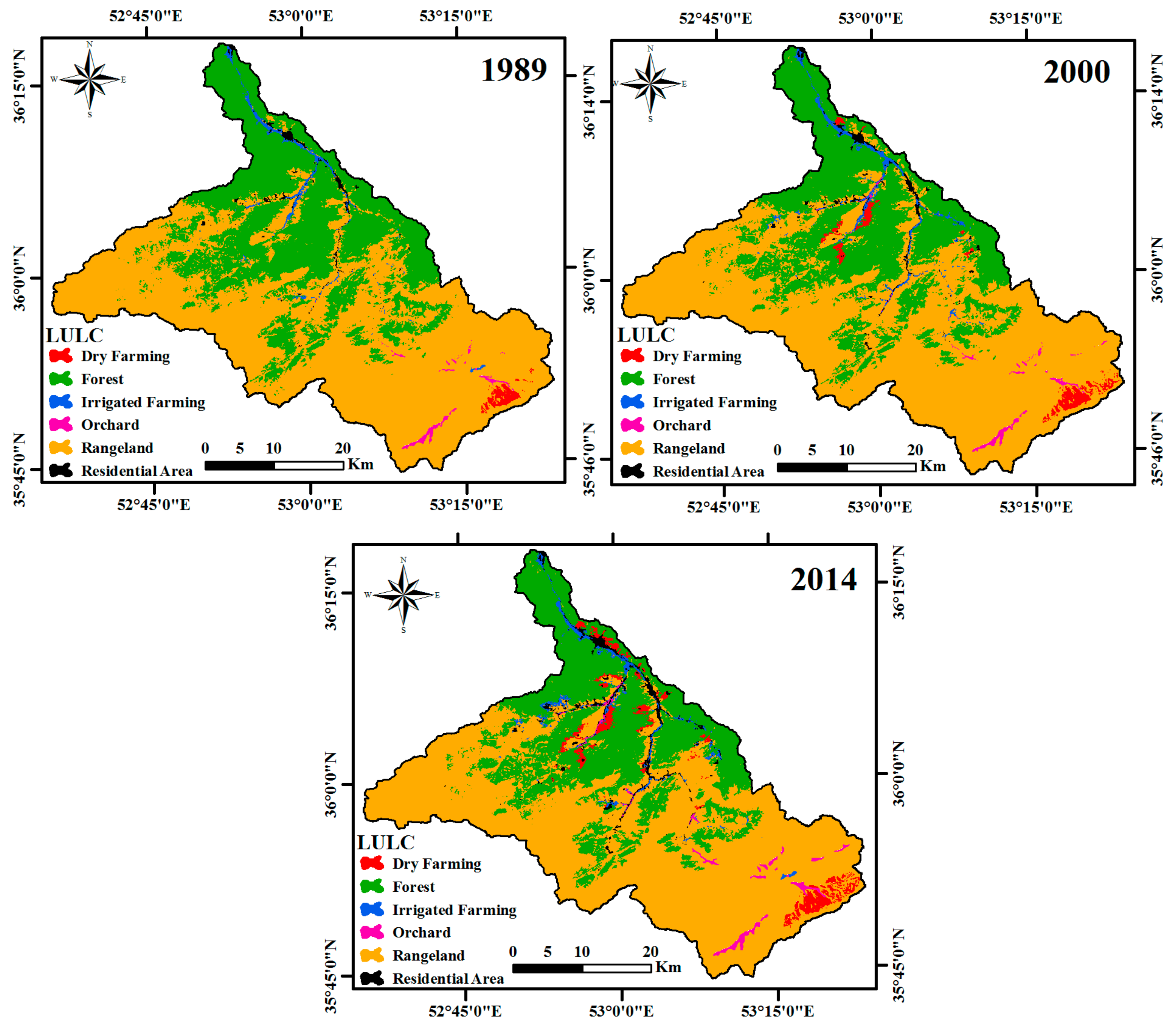
3.1. LULC Map Preparation and Validation

Historical LULC maps of the Talar watershed (1989, 2000, and 2014) and the area of LULC classes in research years are presented in Figure 3 and Table 2, respectively. Based on the findings, a Kappa coefficient of 0.75, 0.77, and 0.82 was obtained for the LULC maps of 1989, 2000, and 2014, respectively. In addition, overall accuracies of 79.51%, 81.15%, and 85.52% were obtained for the LULC maps of 1989, 2000, and 2014, respectively.

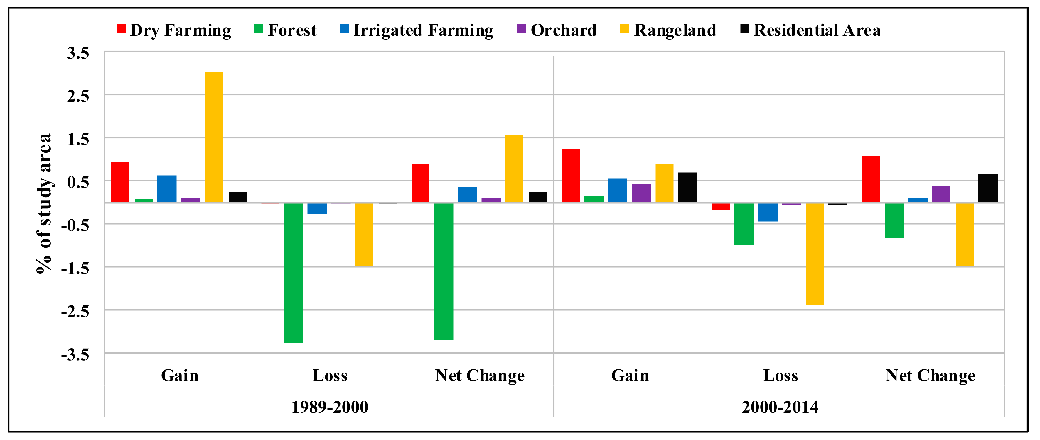
3.2. Change Analysis of LULC Maps

During the study period (1989–2014), the net change area of dry farming, forest, irrigated farming, orchard, rangeland, and residential area were 35.62, −71.02, 8.45, 8.55, 2.3, and 16.27 km2. In addition, 94.92, 94.96, and 92.42% of the Talar watershed persisted in the periods of 1989 to 2000, 2000 to 2014, and 1989 to 2014. Moreover, forest to rangeland, rangeland to dry farming, forest to dry farming, and rangeland to residential area changes had the highest LULC transition area for 1989–2014. Between 1989–2014, a large portion of losses was allocated to forest (73.74 km2) and rangeland (51.57 km2). In addition, the gains of rangeland (53.59 km2), dry farming (36.17 km2) and residential area (16.65 km2) categories are ranked at places 1 to 3 for all changes, respectively. According to our findings, between 1989–2000, the budgeted changes in dry farming, forest, irrigated farming, orchard, rangeland, and residential amount to 0.92, −3.20, 0.35, 0.11, 1.58, and 0.25%, respectively. For 2000–2014, the changes amounted to 1.10, −0.82, 0.13, 0.37, −1.46, 0.67%, respectively. More details of gains, losses, and net changes in each LULC class between 1989 and 2014 are depicted in Figure 4.

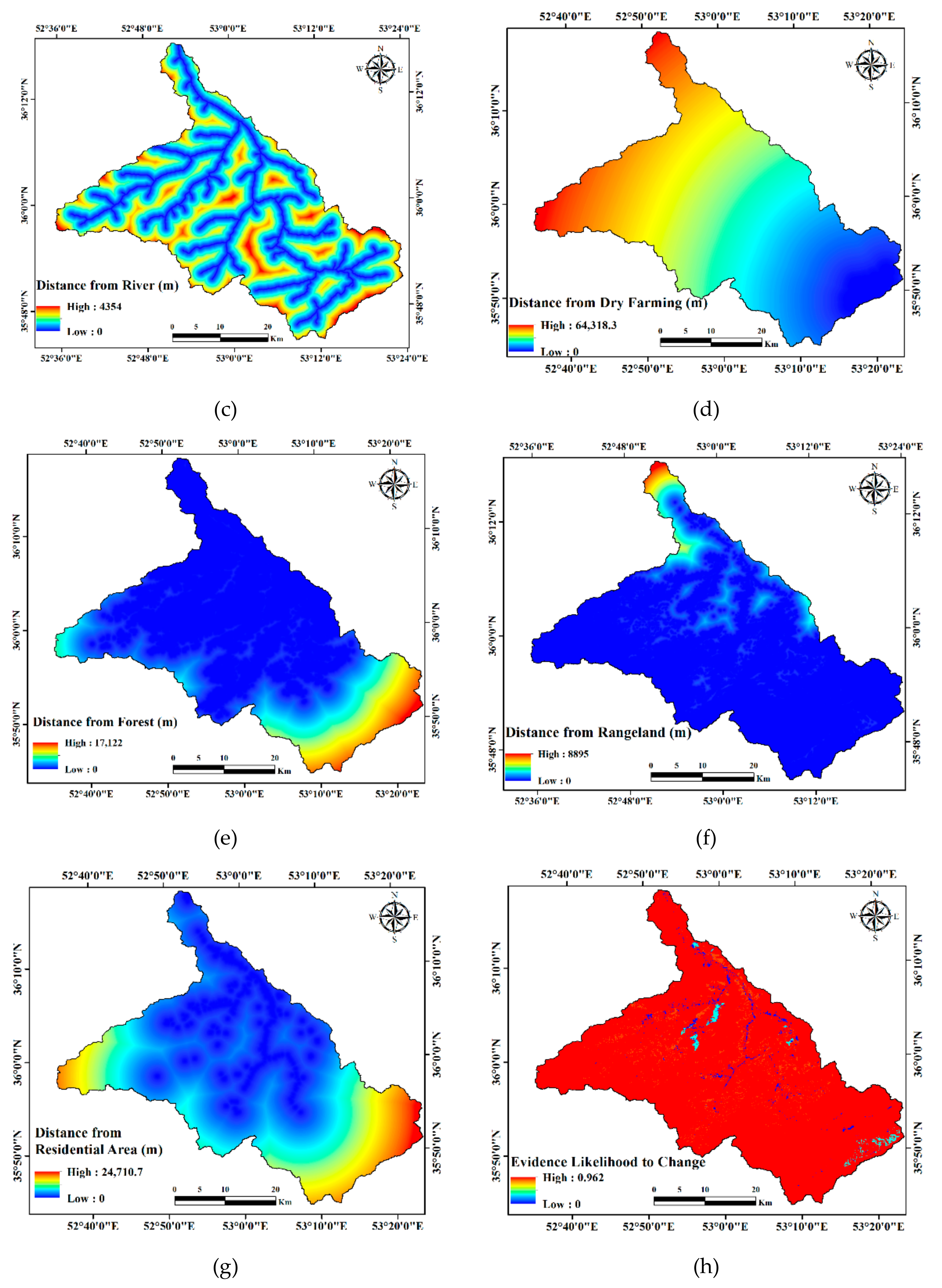
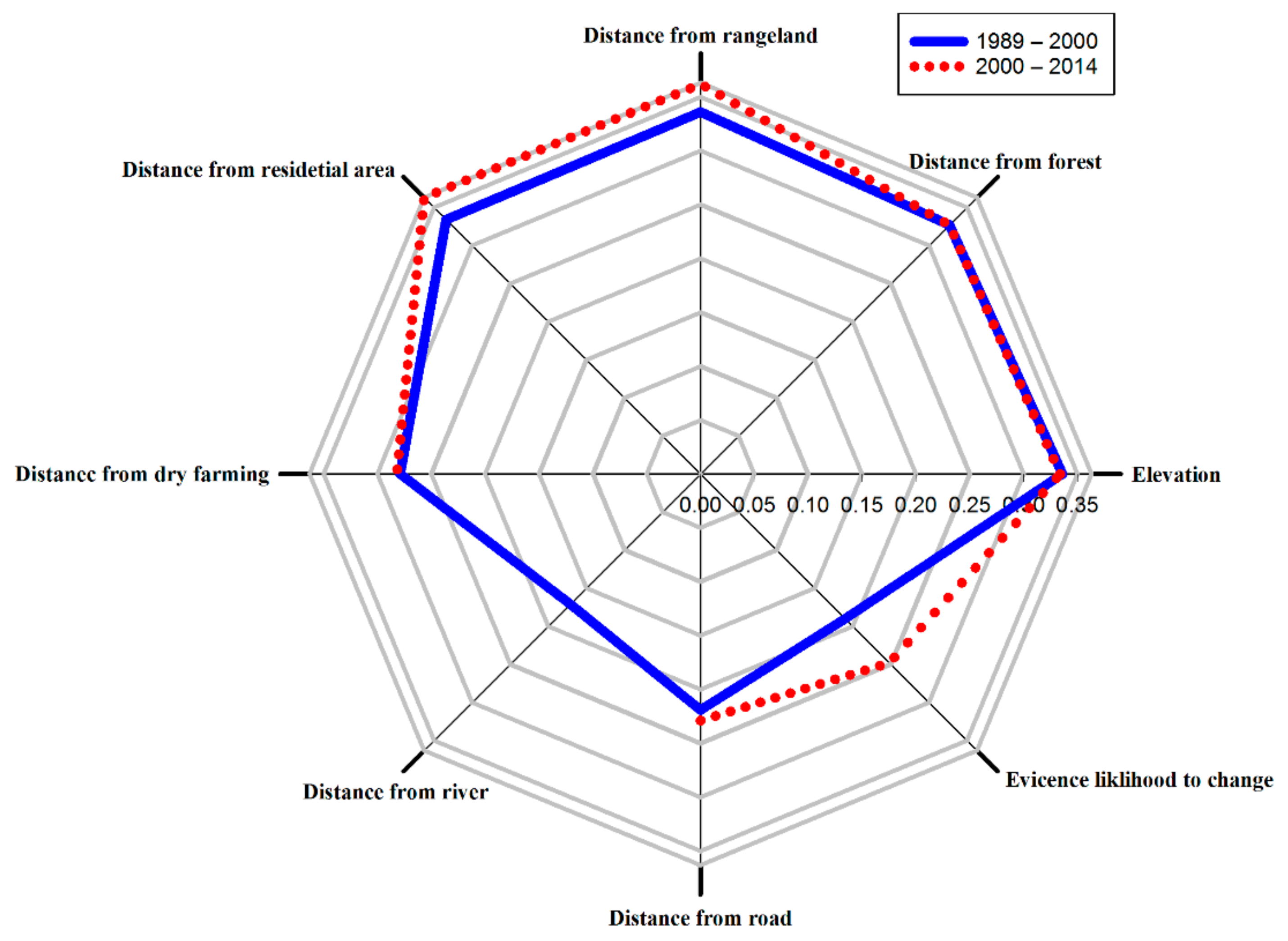
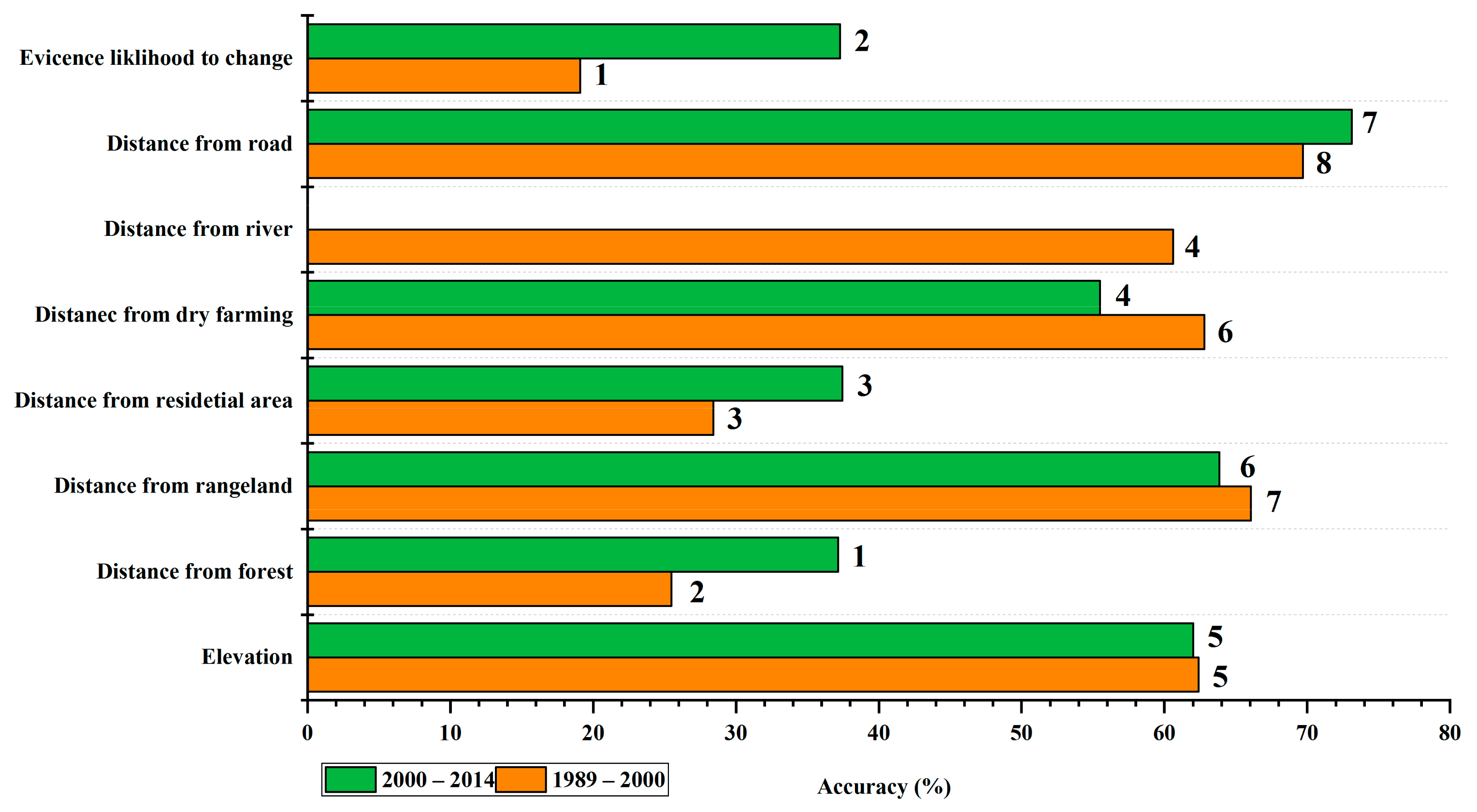
3.3. Transition Potential Modeling

According to the observed LULC changes in the study area, the transition from dry farming to rangeland, forest to dry farming, forest to irrigated farming, forest to rangeland, forest to residential area, irrigated farming to residential area, rangeland to dry farming, rangeland to orchard, and rangeland to residential area were used for transition potential modeling and change prediction of LULC maps for both study periods (1989–2000 and 2000–2014).
The results of explanatory variables mapping to predict the LULC map 2014 are provided in Figure 5a–h. In addition, the finding of Cramer’s V coefficient examination for research periods are illustrated in Figure 6. The maximum and minimum of Cramer’s V coefficient obtained 0.33 (Elevation) and 0.17 (distance from river) for 1989–2000, and 0.36 (Elevation) and 0.22 (distance from road) for 2000–2014, respectively.
The accuracy rate of MLP in transition potential modeling obtained 74.53 and 76.71% for 1989–2000 and 2000–2014, respectively. Training RMS were observed 0.172 and 0.165 for the first and second period of study. In addition, testing RMS were acquired as 0.175 and 0.165 for the research periods, respectively. Figure 7 shows the sensitivity analysis finding of explanatory variables in 1989–2000 and 2000–2014 in the Talar watershed. The ranking of each explanatory factor is also presented inside the histogram.

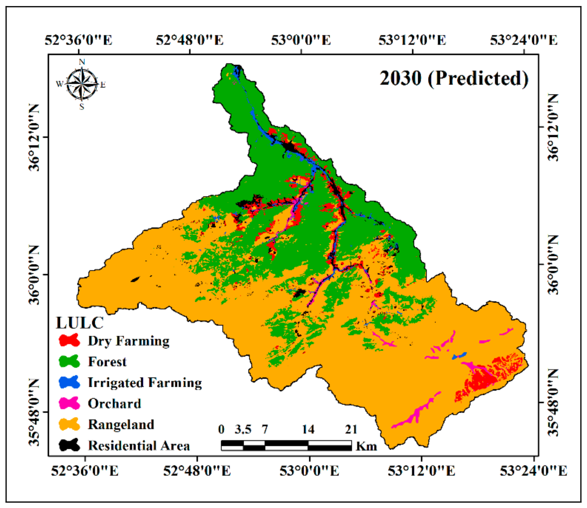
3.4. LULC Change Prediction

The future LULC map of the study watershed was predicted by using the LULC maps of 2000 and 2014 considering the occurred change dynamics (dry farming to rangeland, forest to dry farming, forest to irrigated farming, etc.) in the period of 1989–2000. The predicted LULC map 2030 is shown in Figure 8. In the statistical and visual validation result of the LULC map 2014, Kno and Klocation, and FOM amounted to 0.964, 0.969, and 10.53%, respectively. Based on the prediction results, the area of dry farming, forest, irrigated farming, orchard, rangeland, and residential area will be 66.7, 531.2, 21.1, 22.9, 1080.8, and 41.1 km2 for 2030, respectively.

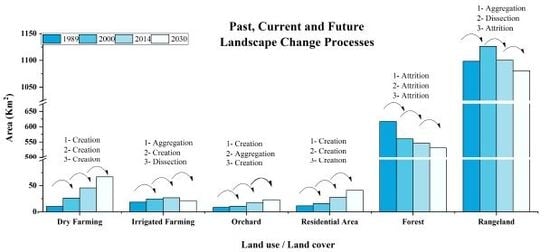
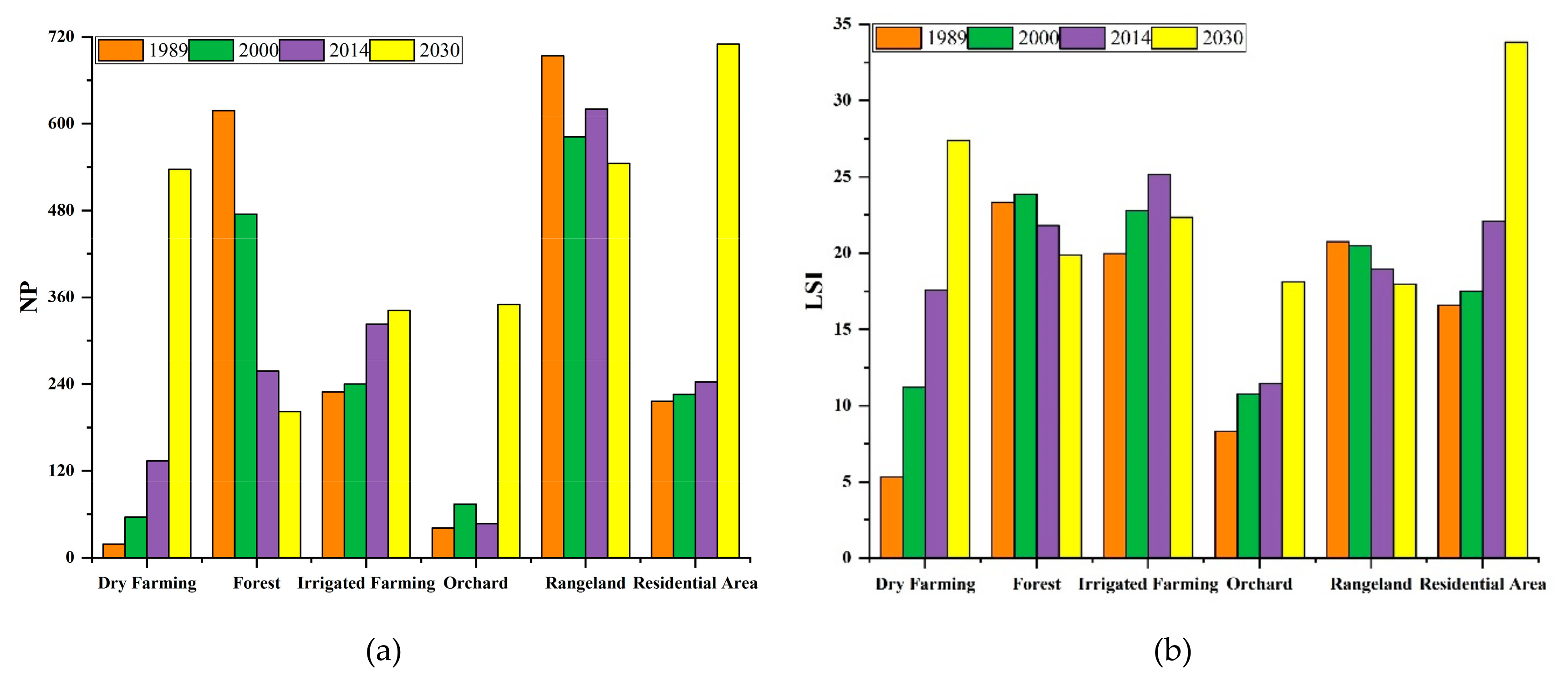
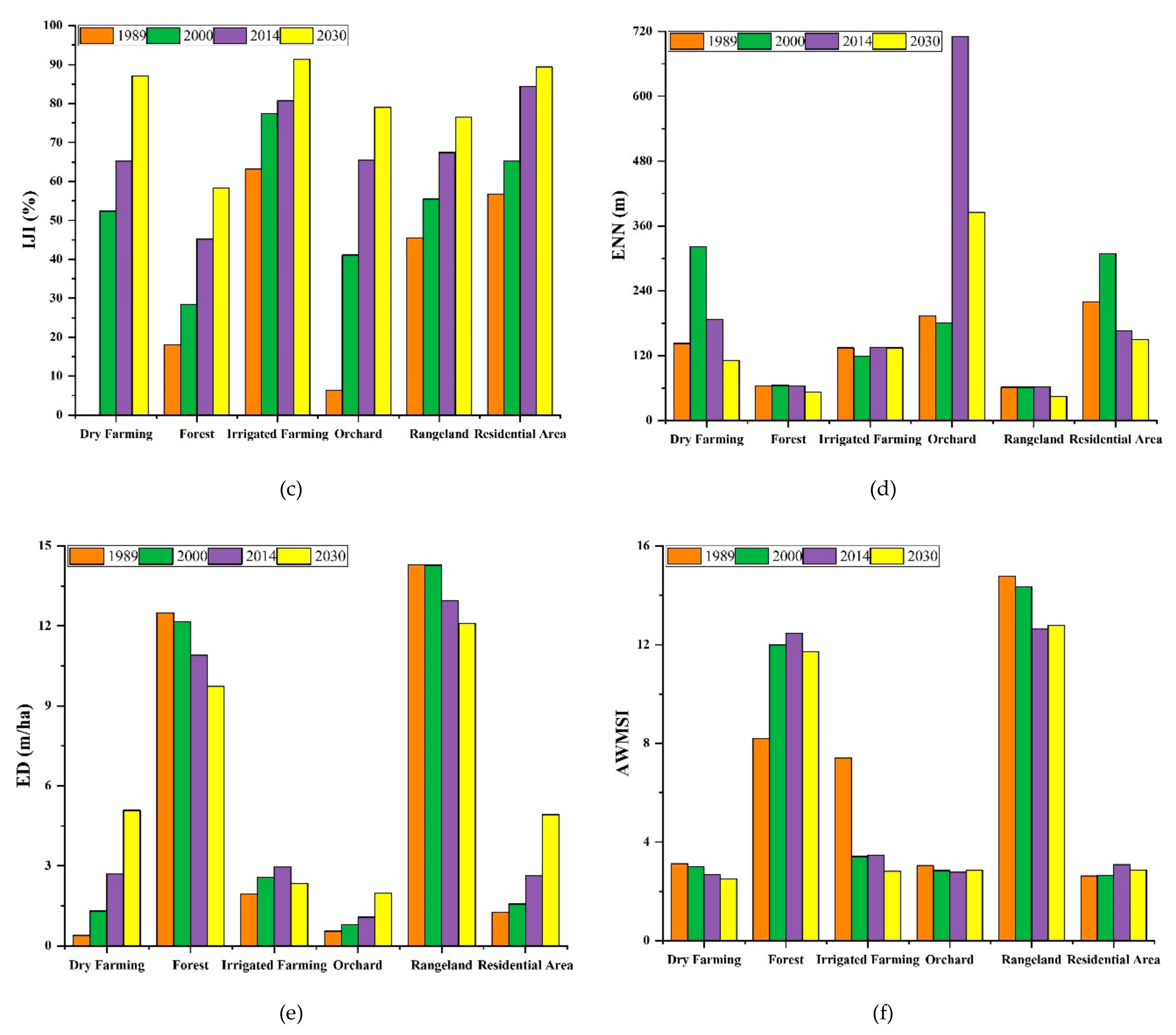
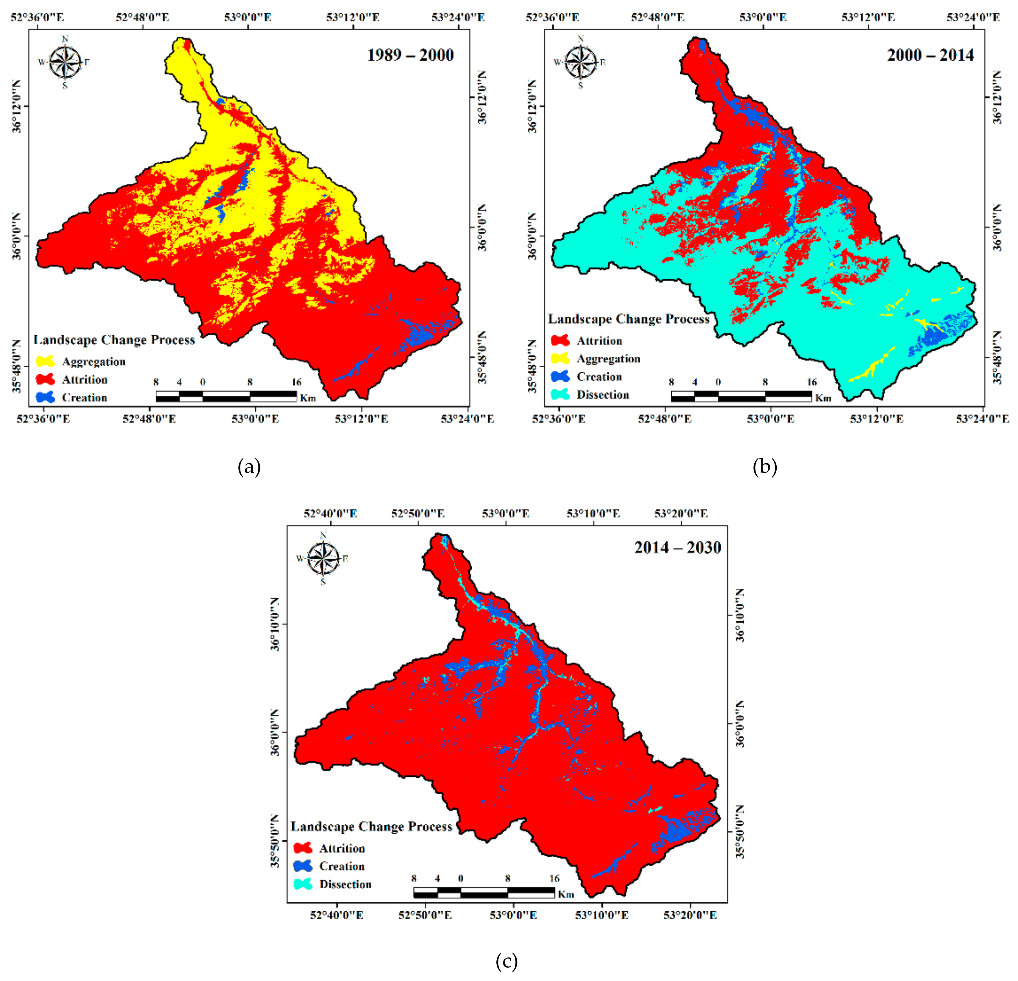
3.5. Investigation of Landscape Metrics and Change Processes

The computation results from LMs metrics including NP, LSI, IJI, ENN, ED, and AWMSI at class and landscape level are indicated in Table 3 and Figure 9a–f.
The prediction results of LMs for 2030 in landscape level illustrate that NP, LSI, IJI, and ED will increase compared to 2014 by approximately 65.3, 7.63, 20.1, and 8.77%, respectively. ENN, and AWMSI will be reduced by −1.35, and 0.61% for the future condition of Talar watershed.
At class level, the number of agriculture (dry and irrigated farming) patches increased from 248 in 1989 to 296 in 2000, and 457 in 2014. During the research period, NP decreased from 618 to 258 and from 694 to 620 for forest and rangeland categories, respectively. The number of patches within the orchard class increased from 41 to 74 and then decreased to 47 for 1989, 2000, and 2014, respectively. The NP of residential areas rose from 216 to 243 for 1989–2014. The NP will be changed to 300.74, −21.70, 5.8, 644.68, −12.09, and 192.18% in 2030 for dry farming, forest, irrigated farming, orchard, rangeland, and residential area, respectively.
Increases in LSI for dry farming, irrigated farming, orchard, and residential area were identified. This metric will be reduced for forest from 23.33 to 21.81, and rangeland from 20.74 to 18.95 in 1989–2014. The change percent of LSI for 2030 will be 55.96, −8.93, −11.10, 58.20, −5.53, and 53.09 for dry farming, forest, irrigated farming, orchard, rangeland, and residential area, respectively.
In the case of IJI, all LULC categories had an increasing trend from 1989 to 2014. Accordingly, the interspersion of LULC patches was done in the Talar watershed. This trend will continue, and the score for IJI in 2030 for dry farming, forest, irrigated farming, orchard, rangeland, and residential area will be 87.05, 58.36, 91.37, 79.05, 76.46, and 89.39, respectively.
The ENN was augmented from 142.25 to 186.65 for dry farming and from 193.17 to 710.08 for orchard in 1989–2014. For the case of residential areas, the ENN diminished from 218.89 to 165.82 in 1989 and 2014. The values of ENN for forest, irrigated farming and rangeland in the considered period were almost constant and were equal to 63, 134, and 61, respectively. The predicted values of this metric for 2030 will be 110.49, 52.23, 134.13, 385.32, 44.78, and 149.54 for dry farming, forest, irrigated farming, orchard, rangeland, and residential area classes.
Increases in ED for dry farming (from 0.38 to 2.70), irrigated farming (from 1.94 to 2.95), orchard (from 0.55 to 1.07), and residential area (from 1.26 to 2.62) were observed for 1989–2014. The ED of forest and rangeland was reduced by 12.63 and 9.35%, respectively, over the research period. The predicted ED shows that the values for 2030 will be 5.07, 9.73, 2.33, 1.97, 12.09, and 4.91 for dry farming, forest, irrigated farming, orchard, rangeland, and residential area, respectively.
Increasing trends of AWMSI are expected for forest (from 8.18 to 12.46) and residential areas (from 2.61 to 3.08). Other LULC categories had a decreasing trend in the research period. The percentage changes until 2030 will be −6.45, −6.02, −18.52, 2.54, 0.95, and −6.94% for dry farming, forest, irrigated farming, orchard, rangeland, and residential area, respectively.
Figure 10a–c illustrates the spatial distribution of LCPs for 1989–2000, 2000–2014, and 2014–2030 in the Talar watershed. In addition, NP, Patch Area (PA), and Patch Perimeter (PP) metrics of each LULC category are provided in the Appendix A for better understanding of the explored change processes.
As shown in Figure 10, four change processes including aggregation, attrition, creation, and dissection were identified for different periods of the research region. In the first period (1989–2000), the Talar watershed experienced the change processes of aggregation (66.15% of study area), attrition (31.75% of study area), and creation (2.08% of study area). Aggregation (0.97% of study area), attrition (30.93% of study area), creation (5.68% of study area), and dissection (62.40% of study area) occurred from 2000 to 2014. Based on the real LULC map of 2014 and the predicted LULC use map of 2030, it is expected that particularly the change processes of attrition, creation, and dissection will continue and even increase.

4. Discussion

4.1. LULC Changes

According to the findings, deforestation, agriculture land development, and residential area expansion with the area of 71.02, 44.08, and 16.27 km2 experienced the most intensive LULC changes in the Talar watershed, respectively. A very similar trend in deforestation (14%) and urban expansion (82%) for southern Minnesota during 1975–2006 was reported by [18]. The change from forest to rangeland and agriculture lands were the most prominent transition pathways in our case study area, which is consistent with results of [9] in the Neka watershed with the 1835 ha deforestation (1987–2001). Global LULCC shows the same alarming trends. For instance, 107.2 km2 of the Bhanupratappur Forest Division in India were deforested in 1990–2010 [31], and 71,325 ha of forests in Sub-Saharan Africa between 1975–2000 [47] were deforested and degraded. [48] observed the same trend of agricultural expansion in the expanses of forests and rangelands (1929–1955) in the Basilicata, southern Italy. Vice versa, less suitable soils and less productive agriculture lands in southern Minnesota led to losses in agricultural area [18] and could be assumed to be an alternative scenario for the future development in the Talar watershed if soil degradation is going on. The occurrence of destructive floods [19], illegal logging, and overgrazing are controversy processes that will decide upon the sustainable future development of the watershed.

4.2. Transition Potential Modeling

Cramer’s V coefficient results (Figure 6) illustrated that the distance from rangeland (0.36) and the distance from residential area (0.36) had the highest explanatory value for the LULC transition in 2000–2014. The minimum value of Cramer’s V coefficient (0.22) was assigned to the distance from roads. This is contradictory to findings from [49] for the deforestation in tropical areas. The pressures of urban sprawl seemed to be the more relevant phenomenon in the Talar watershed. These results confirm the findings of [31] in India and [50] in the Gaza Strip. Elevation with a value of 0.34 for Cramer’s V coefficient can play an important role in transition potential modeling, which is also confirmed by [40] for the Haraz watershed, Iran. The accuracy assessment of transition potential modeling indicated a good performance with the obtained accuracy rate for the two considered periods (74.53 and 76.71% for 1989–2000 and 2000–2014, respectively).

4.3. LULC Change Prediction

There is a possibility of an error in identifying and evaluating changes in statistical procedures [49]. The statistical assessment of the predicted LULC map 2014 in the Talar watershed revealed good performance. The overall accuracy and the level of agreement of location as Kno and Klocation obtained 0.964 and 0.969, respectively, which is higher than values published by [39] in the Arak Metropolitan Area and [51] for similar studies in the Greater Cairo region of Egypt. Based on the findings of the visual assessment of the predicted LULC map 2014, the values of hits, null successes, false alarms, and misses obtained 0.86, 91.75, 4.43, and 2.94%, respectively. Accordingly, FOM was calculated to amount to 10.53%. The acquired FOM is higher than values of 10.4 and 2.9% obtained in [52] and [53] studies in the Spanish autonomous community of Murcia and the Colombian Andes region, respectively.

4.4. Investigation of Landscape Metrics and Change Processes

Based on the findings, all considered LMs except NP and AWMSI had an increasing trend at the landscape level over the study period (1989–2014) in the Talar watershed (Table 3). Similar results were achieved by [18] in their case study in southern Minnesota. [9] reported an increasing trend in NP and AWMSI in the Neka watershed, which is not consistent with our findings. Increases in NP and LSI in all LULC categories except forest and rangeland during the study period indicated the progressing trend of fragmentation, shape irregularity, and complexity of patches in the considered LULC classes. Based on the LULC reform of Iran in 1963 [54], the ownership of lands was changed from feudal to peasant, which increased the number and area of agricultural patches, and then led to many environmental problems. The obtained results of this research can be seen as an alarm to avoid past mistakes. In addition, a need to increase the potential of dry farming, irrigated farming, orchard, and residential area patches to change over a 25-years research period based on the investigation of ED can be deduced. A rising trend of NP, LSI, and ED in agriculture lands, orchard, and residential area categories demonstrates the impact of human activities on landscape change in the Talar watershed. Interspersion and juxtaposition of patches were rising in all studied LULC classes in the research period. Monitoring of IJI metrics for 1989–2014 designated the progressing variations in patches adjacent to other LULC classes in the Talar watershed, which led to more complexity of the landscape. According to our obtained results of ENN, only the residential area has been decreasing from 1989 to 2014. The rising trend of ENN for dry farming, and orchard classes depicted a change in the distribution from dense clumps to scattered patches. In the case of AWMSI, forest and residential area became more complex, more diverse, and more sensitive to fragmentation [15] for 1989–2014. The remaining LULC categories had a reducing trend in AWMSI, which was leading to more simple shapes. Although LMs provide useful information regarding landscape patterns and help decision-makers to accomplish better planning, they have some limitations. The attributes and behavior of LMs may not determine the relationship between LMs and ecological or hydrological processes [53]. The research conclusion of [55] illustrated that none of the LMs are suitable for all aspects of a landscape analysis, and special attention should be paid to the value of LMs and ecological processes. [56] stated that the interpretation of LMs is only feasible when the restrictions of each metric are completely identified. In addition, some LMs do not provide information on patch distribution [42]. [57] noted that the dynamics of landscape patches have some limitations and cannot be adequately ascertained. It is therefore recommended to conduct the landscape change detection in a holistic spatial framework [18,58], which can be achieved by the use of LCPs as a key concept provided through landscape ecology. The temporal investigation of landscape changes in the Talar watershed showed that the type of occurred change processes was not completely the same in the studied periods (1989–2000 and 2000–2014). Nevertheless, aggregation, attrition, and creation happened for both periods of 1989–2000 and 2000–2014. The change process of creation was observed for dry farming in two study periods. Decreasing trend of NP, PA, and PP led to an attrition change process for the forest category in the Talar watershed through a reduction in the area (from 617.12 to 546.10) and the number of forest patches (from 681 to 276) over a 25-year research period (1989–2014). The irrigated farming class experienced the change processes of aggregation and creation for 1989 to 2000 and 2000 to 2014 periods, respectively. Creation and aggregation were two identified LCPs in the first and second research period for the orchard category in the Talar watershed. In the case of rangeland, the explored change processes were aggregation and dissection for 1989–2000 and 2000–2014, respectively. The change process of creation was identified for residential areas for two research periods. According to the findings, the future LCPs of attrition, creation, and dissection will increase in the Talar watershed. In detail, the predicted change processes are creation in dry farming, orchard, and residential classes, attrition in forest and rangeland categories, and dissection in irrigated farming by 2030. The dynamics of LMs and also LCPs combined in one analytical framework can facilitate the understanding and detection of the relationship between ecological processes and landscape patterns that open up new opportunities for interpreting better critical LULC change.

5. Conclusions

Deforestation, agriculture land development, and residential area expansion occurred in 71.02, 44.07, and 16.26 km2 of the Talar watershed, which had consequences such as destructive flooding in 2012. According to our findings, although complexity and disorganization of given LULC classes have increased, this situation is more evident in agriculture, orchard, and residential area categories during 1989–2014, which were put under increasing pressures by human activities. This situation is governing in most of the watersheds in northern Iran. Thus, the results are widely transferrable in the similar regions in term of LULC pattern, utilization style, affecting forces on LULC change, and similar change type at national scale. Comparable change process can be interpreted using these findings considering the changes in the LULC over consecutive time spans. The ownership changes in lands (especially agricultural lands) in the extensive LULC reform law of Iran in 1963 led to an increase in agricultural lands that caused many environmental problems. With regard to the experience of the LULC reform law in Iran, the results are alarming. Trying to revise deterrent laws for LULC change in order to achieve environmental sustainability with consideration of legal and illegal LULC changes is a positive implication for the present study. Actors governing LULC management and planning should pay attention to the landscape ecology and all aspects of future landscape change including the change in ecosystems services, health, and sustainability. With due attention to results from current research, a roadmap for improved LULC management and planning in the Talar watershed will be provided.

Author Contributions

Conceptualization: M.Z., H.M., M.G., A.K.D., and C.F.; methodology: M.Z., M.G., and C.F.; validation: M.Z., H.M., C.F.; formal analysis: M.Z., and A.K.D.; investigation: M.Z., H.M., M.G., A.K.D., and C.F.; writing—original draft preparation: M.Z.; writing-review and editing: C.F., and M.G.; visualization: M.Z.; supervision: H.M., and C.F. All authors have read and agreed to the published version of the manuscript.

Funding

This research received no external funding.

Acknowledgments

We would like to appreciate the ministry of science, research and technology of Iran for supporting the sabbatical of the first author and the department of sustainable landscape development of Martin Luther University Halle-Wittenberg, Germany for providing an adequate working environment.

Conflicts of Interest

The authors declare no conflict of interest.

Appendix A

Table A1. The extraction result of change processes in different LULC categories for different study periods.
PeriodLUChange ProcessNPPAPP
1989–2000Dry FarmingCreation195611,28329,28022647682
ForestAttrition618475685,319622,50877,29075,312
Irrigated FarmingAggregation22924020,49127,34511,45815,076
OrchardCreation4174948711,63432404640
RangelandAggregation6945821,220,9381,251,89091,71091,686
Residential AreaCreation21622812,61517,47674609278
2000–2014Dry FarmingCreation5613429,28050,854768215,882
ForestAttrition475258622,508606,38375,31267,966
Irrigated FarmingCreation24032327,34529,90815,07617,392
OrchardAggregation744711,63419,11446406348
RangelandDissection5826201,251,8901,223,18391,68683,870
Residential AreaCreation22824317,47630,691927815,512
2014–2030Dry FarmingCreation13453750,85474,20515,88229,866
ForestAttrition258202606,383590,32267,96661,062
Irrigated FarmingDissection32334229,90823,54317,39213,718
OrchardCreation4735019,11425,446634811,602
RangelandAttrition6205451,223,1831,200,87983,87078,664
Residential AreaCreation24371030,69145,68815,51228,958

References

  1. Chen, L.; Fu, B.; Xu, J.; Gong, J. Location-weighted landscape contrast index: A scale independent approach for landscape pattern evaluation based on source-sink ecological processes. Acta Ecol. Sin. 2003, 23, 2406–2413. [Google Scholar]
  2. Girvetz, E.H.; Thorne, J.H.; Berry, A.M.; Jaeger, J.A.G. Integration of landscape fragmentation analysis into regional planning: A statewide multi-scale case study from California, USA. Landsc. Urban Plan. 2008, 86, 205–218. [Google Scholar] [CrossRef]
  3. Hu, Y.; Zheng, Y.; Zheng, X. Simulation of land-use scenarios for Beijing using CLUE-S and Markov composite models. Chin. Geogr. Sci. 2013, 23, 92–100. [Google Scholar] [CrossRef]
  4. Kleemann, J.; Baysal, G.; Bulley, H.N.N.; Fürst, C. Assessing driving forces of land use and land cover change by a mixed-method approach in north-eastern Ghana, West Africa. J. Environ. Manag. 2017, 196, 411–442. [Google Scholar] [CrossRef] [PubMed]
  5. Ai, L.; Shi, Z.H.; Yin, W.; Huang, X. Spatial and seasonal patterns in stream water contamination across mountainous watersheds: Linkage with landscape characteristics. J. Hydrol. 2015, 523, 398–408. [Google Scholar] [CrossRef]
  6. Xystrakis, F.; Psarras, T.; Koutsias, N. A process-based land use/land cover change assessment on a mountainous area of Greece during 1945–2009: Signs of socio-economic drivers. Sci. Total Environ. 2017, 587–588, 360–370. [Google Scholar] [CrossRef]
  7. Inkoom, J.N.; Frank, S.; Greve, K.; Walz, U.; Fürst, C. Suitability of different landscape metrics for the assessments of patchy landscapes in West Africa. Ecol. Indic. 2018, 85, 117–127. [Google Scholar] [CrossRef]
  8. Nor, A.N.M.; Corstanje, R.; Harris, J.A.; Brewer, T. Impact of rapid urban expansion on green space structure. Ecol. Indic. 2017, 81, 274–284. [Google Scholar] [CrossRef]
  9. Shooshtari, S.J.; Gholamalifard, M. Scenario-based land cover change modeling and its implications for landscape pattern analysis in the Neka Watershed, Iran. Remote Sens. Appl. Soc. Environ. 2015, 1, 1–19. [Google Scholar] [CrossRef]
  10. Krajewski, P.; Solecka, I.; Mrozik, K. Forest landscape change and preliminary study on its driving forces in ślȩza landscape park (Southwestern Poland) in 1883–2013. Sustainability 2018, 10, 4526. [Google Scholar] [CrossRef] [Green Version]
  11. Mayer, A.L.; Buma, B.; Davis, A.D.; GagnCrossed, D.; Sign, S.A.; Louise Loudermilk, E.; Scheller, R.M.; Schmiegelow, F.K.A.; Wiersma, Y.F.; Franklin, J. How Landscape Ecology Informs Global Land-Change Science and Policy. Bioscience 2016, 66, 458–469. [Google Scholar] [CrossRef] [Green Version]
  12. Potschin, M.B.; Haines-Young, R.H. Landscapes and sustainability. Landsc. Urban Plan. 2006, 3, 155–161. [Google Scholar] [CrossRef]
  13. Lausch, A.; Herzog, F. Applicability of landscape metrics for the monitoring of landscape change: Issues of scale, resolution and interpretability. Ecol. Indic. 2002, 2, 3–15. [Google Scholar] [CrossRef]
  14. Leitao, A.B.; Ahern, J. Applying landscape ecological concepts and metrics in sustainable landscape planning. Landsc. Urban Plan. 2002, 59, 65–93. [Google Scholar] [CrossRef]
  15. Lee, S.W.; Hwang, S.J.; Lee, S.B.; Hwang, H.S.; Sung, H.C. Landscape ecological approach to the relationships of land use patterns in watersheds to water quality characteristics. Landsc. Urban Plan. 2009, 92, 80–89. [Google Scholar] [CrossRef]
  16. Gergel, S.E.; Turner, M.G.; Miller, J.R.; Melack, J.M.; Stanley, E.H. Landscape indicators of human impacts to riverine systems. Aquat. Sci. 2002, 64, 118–128. [Google Scholar] [CrossRef]
  17. Uuemaa, E.; Antrop, M.; Marja, R.; Roosaare, J.; Mander, Ü. Landscape Metrics and Indices: An Overview of Their Use in Landscape Research Imprint / Terms of Use. Living Rev. Landsc. Res. 2009, 3, 1–28. [Google Scholar] [CrossRef]
  18. Paudel, S.; Yuan, F. Assessing landscape changes and dynamics using patch analysis and GIS modeling. Int. J. Appl. Earth Obs. Geoinf. 2012, 16, 66–76. [Google Scholar] [CrossRef]
  19. Motevalli, A.; Vafakhah, M. Flood hazard mapping using synthesis hydraulic and geomorphic properties at watershed scale. Stoch. Environ. Res. Risk Assess. 2016, 30, 1889–1900. [Google Scholar] [CrossRef]
  20. Neel, M.C.; McGarigal, K.; Cushman, S.A. Behavior of class-level landscape metrics across gradients of class aggregation and area. Landsc. Ecol. 2004, 19, 435–455. [Google Scholar] [CrossRef]
  21. Bianchin, S.; Richert, E.; Heilmeier, H.; Merta, M.; Seidler, C. Landscape metrics as a tool for evaluating scenarios for flood prevention and nature conservation. Landsc. Online 2011, 25, 1–15. [Google Scholar] [CrossRef]
  22. Toutakhane, A.; Mofareh, M. Investigation and Evaluation of Spatial Patterns in Tabriz Parks Using Landscape Metrics. J. Urban Environ. Eng. 2016, 10, 263–269. [Google Scholar] [CrossRef]
  23. Maghsood, F.F.; Moradi, H.; Bavani, A.R.M.; Panahi, M.; Berndtsson, R.; Hashemi, H. Climate change impact on flood frequency and source area in northern Iran under CMIP5 scenarios. Water (Switz.) 2019, 11, 273. [Google Scholar] [CrossRef] [Green Version]
  24. Shooshtari, S.J.; Shayesteh, K.; Gholamalifard, M.; Azari, M.; López-Moreno, J.I.; Interactions, H.A.; Dei, C.D.A. Land cover change modelling in Hyrcanian forests, northern Iran: A landscape pattern and transformation analysis perspective. Cuad. Investig. Geogr. 2018, 44, 743–761. [Google Scholar] [CrossRef] [Green Version]
  25. Poorzady, M.; Bakhtiari, F. Spatial and temporal changes of Hyrcanian forest in Iran. iForest-Biogeosciences For. 2009, 2, 198. [Google Scholar] [CrossRef]
  26. Rozenstein, O.; Karnieli, A. Comparison of methods for land-use classification incorporating remote sensing and GIS inputs. Appl. Geogr. 2011, 31, 533–544. [Google Scholar] [CrossRef]
  27. Yousefi, S.; Khatami, R.; Mountrakis, G.; Mirzaee, S.; Pourghasemi, H.R.; Tazeh, M. Accuracy assessment of land cover/land use classifiers in dry and humid areas of Iran. Environ. Monit. Assess. 2015, 187, 641. [Google Scholar] [CrossRef]
  28. Congalton, R.G. A review of assessing the accuracy of classifications of remotely sensed data. Remote Sens. Environ. 1991, 37, 35–46. [Google Scholar] [CrossRef]
  29. Bakr, N.; Weindorf, D.C.; Bahnassy, M.H.; Marei, S.M.; El-Badawi, M.M. Monitoring land cover changes in a newly reclaimed area of Egypt using multi-temporal Landsat data. Appl. Geogr. 2010, 30, 592–605. [Google Scholar] [CrossRef]
  30. Eastman, J.R. TerrSet manual. Access. TerrSet Version 2015, 18, 1–390. [Google Scholar]
  31. Kumar, S.; Radhakrishnan, N.; Mathew, S. Land use change modelling using a Markov model and remote sensing. Geom. Nat. Hazards Risk 2014, 5, 145–156. [Google Scholar] [CrossRef]
  32. Pistocchi, A.; Luzi, L.; Napolitano, P. The use of predictive modeling techniques for optimal exploitation of spatial databases: A case study in landslide hazard mapping with expert system-like methods. Environ. Geol. 2002, 41, 765–775. [Google Scholar] [CrossRef]
  33. Mountrakis, G.; Im, J.; Ogole, C. Support vector machines in remote sensing: A review. ISPRS J. Photogramm. Remote Sens. 2011, 66, 247–259. [Google Scholar] [CrossRef]
  34. Mishra, V.; Rai, P.; Mohan, K. Prediction of land use changes based on land change modeler (LCM) using remote sensing: A case study of Muzaffarpur (Bihar), India. J. Geogr. Inst. Jovan Cvijic SASA 2014, 64, 111–127. [Google Scholar] [CrossRef]
  35. Hamdy, O.; Zhao, S.A.; Salheen, M.; Eid, Y.Y. Analyses the Driving Forces for Urban Growth by Using IDRISI®Selva Models Abouelreesh—Aswan as a Case Study. Int. J. Eng. Technol. 2017, 9, 226–232. [Google Scholar] [CrossRef] [Green Version]
  36. Romano, G.; Abdelwahab, O.M.M.; Gentile, F. Modeling land use changes and their impact on sediment load in a Mediterranean watershed. Catena 2018, 163, 342–353. [Google Scholar] [CrossRef]
  37. Chen, H.; Pontius, R.G. Diagnostic tools to evaluate a spatial land change projection along a gradient of an explanatory variable. Landsc. Ecol. 2010, 25, 1319–1331. [Google Scholar] [CrossRef]
  38. Liu, T.; Yang, X. Monitoring land changes in an urban area using satellite imagery, GIS and landscape metrics. Appl. Geogr. 2015, 56, 42–54. [Google Scholar] [CrossRef]
  39. Nadoushan, M.A.; Soffianian, A.; Alebrahim, A. Predicting urban expansion in arak metropolitan area using two land change models. World Appl. Sci. J. 2012, 18, 1124–1132. [Google Scholar]
  40. Kavian, A.; Golshan, M.; Abdollahi, Z. Flow discharge simulation based on land use change predictions. Environ. Earth Sci. 2017, 76, 588. [Google Scholar] [CrossRef]
  41. Plexida, S.G.; Sfougaris, A.I.; Ispikoudis, I.P.; Papanastasis, V.P. Selecting landscape metrics as indicators of spatial heterogeneity—A comparison among Greek landscapes. Int. J. Appl. Earth Obs. Geoinf. 2014, 26, 26–35. [Google Scholar] [CrossRef]
  42. McGarigal, K.; Cushman, S.A.; Neel, M.C.; Ene, E. FRAGSTATS: Spatial Pattern Analysis Program for Categorical Maps. Available online: https://www.umass.edu/landeco/research/fragstats/downloads/fragstats_downloads.html (accessed on 22 February 2020).
  43. Dezhkam, S.; Jabbarian, A.B.; Darvishsefat, A.A.; Sakieh, Y. Performance evaluation of land change simulation models using landscape metrics. Geocarto Int. 2017, 32, 655–677. [Google Scholar] [CrossRef]
  44. Frank, S.; Fürst, C.; Lorz, C.; Koschke, L.; Abiy, M.; Makeschin, F. Chances and limits of using landscape metrics within the interactive planning tool Pimp Your Landscape. In Proceedings of the 2010 International Conference on Integrative Landscape Modelling, Montpellier, France, 3–5 February 2010. [Google Scholar]
  45. Turner, M.G.; Gardner, R.H.; O’neill, R.V. Landscape Ecology in Theory and Practice; Springer: Berlin/Heidelberg, Germany, 2001. [Google Scholar]
  46. Bogaert, J.; Ceulemans, R.; Salvador-Van Eysenrode, D. Decision Tree Algorithm for Detection of Spatial Processes in Landscape Transformation. Environ. Manag. 2004, 33, 62–73. [Google Scholar] [CrossRef] [PubMed]
  47. Brink, A.B.; Eva, H.D. Monitoring 25 years of land cover change dynamics in Africa: A sample based remote sensing approach. Appl. Geogr. 2009, 29, 501–512. [Google Scholar] [CrossRef]
  48. Statuto, D.; Cillis, G.; Picuno, P. Analysis of the effects of agricultural land use change on rural environment and landscape through historical cartography and GIS tools. J. Agric. Eng. 2016, 47, 28–39. [Google Scholar] [CrossRef] [Green Version]
  49. Geist, H.J.; Lambin, E.F. Proximate Causes and Underlying Driving Forces of Tropical Deforestation. Bioscience 2002, 52, 143–150. [Google Scholar] [CrossRef]
  50. Abuelaish, B.; Olmedo, M.T.C. Scenario of land use and land cover change in the Gaza Strip using remote sensing and GIS models. Arab. J. Geosci. 2016, 274, 1–14. [Google Scholar] [CrossRef] [Green Version]
  51. Megahed, Y.; Cabral, P.; Silva, J.; Caetano, M. Land Cover Mapping Analysis and Urban Growth Modelling Using Remote Sensing Techniques in Greater Cairo Region-Egypt. ISPRS Int. J. Geo Inform. 2015, 4, 1750–1769. [Google Scholar] [CrossRef] [Green Version]
  52. Camacho Olmedo, M.T.; Paegelow, M.; Mas, J.F. Interest in intermediate soft-classified maps in land change model validation: Suitability versus transition potential. Int. J. Geogr. Inf. Sci. 2013, 27, 2343–2361. [Google Scholar] [CrossRef]
  53. Rodríguez, N.; Armenteras, D.; Retana, J. Land use and land cover change in the Colombian Andes: Dynamics and future scenarios. J. Land Use Sci. 2012, 8, 1–21. [Google Scholar] [CrossRef]
  54. Lenczowski, G. Iran under the Pahlavis; Hoover Institution Press: Stanford, CA, USA, 1978. [Google Scholar]
  55. Li, X.; He, H.S.; Bu, R.; Wen, Q.; Chang, Y.; Hu, Y.; Li, Y. The adequacy of different landscape metrics for various landscape patterns. Pattern Recognit. 2005, 38, 2626–2638. [Google Scholar] [CrossRef]
  56. Hargis, C.; Bissonette, J.; David, J. The behavior of landscape metrics commonly used in the study of habitat fragmentation. Landsc. Ecol. 1998, 13, 167–186. [Google Scholar] [CrossRef]
  57. Dinar, A.; Campbell, M.B.; Zilberman, D. Adoption of improved irrigation and drainage reduction technologies under limiting environmental conditions. Environ. Resour. Econ. 1992, 2, 373–398. [Google Scholar] [CrossRef]
  58. Sudhira, H.S.; Ramachandra, T.V.; Jagadish, K.S. Urban sprawl: Metrics, dynamics and modelling using GIS. Int. J. Appl. Earth Obs. Geoinf. 2004, 5, 29–39. [Google Scholar] [CrossRef]
Figure 1. Flowchart of the present research.
Sustainability 12 01753 g001
Figure 2. Geographical location of the Talar watershed in the world and Iran.
Sustainability 12 01753 g002
Figure 3. Produced land use/land cover (LULC) maps of the Talar Watershed in studied years.
Sustainability 12 01753 g003
Figure 4. Gains, losses, and net changes of each LULC category for 1989–2000 and 2000–2014 in the Talar watershed.
Sustainability 12 01753 g004
Figure 5. Explanatory factors of LULC change including (a) elevation, (b) distance from road, (c) distance from river, (d) distance from dry farming, (e) distance from forest, (f) distance from rangeland, (g) distance from residential area, and (h) evidence likelihood to change for 1989–2000 in the Talar watershed.
Sustainability 12 01753 g005aSustainability 12 01753 g005b
Figure 6. The Cramer’s V coefficient values of considered explanatory variables for study periods.
Sustainability 12 01753 g006
Figure 7. Sensitivity analysis results of explanatory variables in Talar watershed.
Sustainability 12 01753 g007
Figure 8. Predicted LULC map 2030 in the Talar watershed.
Sustainability 12 01753 g008
Figure 9. The results from landscape metrics calculations including (a) number of patches, (b) landscape shape index, (c) interspersion and juxtaposition index, (d) Euclidean nearest-neighbor distance, (e) edge density, and (f) area-weighted shape index in class level in the Talar watershed.
Sustainability 12 01753 g009aSustainability 12 01753 g009b
Figure 10. Landscape change processes for the research periods of (a) 1989–2000, (b) 2000–2014, and (c) 2014–2030 in the Talar watershed.
Sustainability 12 01753 g010
Table 1. Definition of landscape change processes.
No.Change ProcessDescription
1DeformationThe shape is changing
2ShiftThe position is changing
3PerforationThe number of patches is constant, but the area is decreasing
4ShrinkageThe area and perimeter are decreasing, but the number of patches is constant
5EnlargementThe number of patches is constant, but the area is increasing
6AttritionThe number of patches and area are decreasing
7AggregationThe number of patches is decreasing, but area is constant or increasing
8CreationThe number of patches and area are increasing
9DissectionThe number of patches is increasing and the area is decreasing
10FragmentationThe number of patches is increasing and the area is strongly decreasing
Table 2. The area of LULC classes (km2) in research years.
LU198920002014
Area%Area%Area%
Dry Farming10.170.5826.331.4945.792.60
Forest617.1234.98560.6031.78546.1030.96
Irrigated Farming18.451.0524.591.3926.901.52
Orchard8.630.4910.600.6017.170.97
Rangeland1098.3962.261126.2663.841100.5262.38
Residential11.360.6415.740.8927.621.57
Table 3. The results from metrics calculations in landscape levels in the Talar watershed.
Year NP LSI IJI ENN ED AWMSI
1989181718.3037.6765.0115.4512.19
2000165519.2150.1970.1016.3213.10
2014162519.5165.5574.8316.6011.94
2030259520.9978.7174.3718.0611.78

