Article

A Stochastic Dominance Approach to Evaluating Pro-Poor Growth—An Application to the Spanish Case

1
Department of Economics, University of Alcalá, 28802 Alcalá de Henares, Spain
2
Department of Applied Economics, University of Valladolid, 47011 Valladolid, Spain
*
Author to whom correspondence should be addressed.
Sustainability 2020, 12(5), 1728; https://doi.org/10.3390/su12051728
Submission received: 23 January 2020 / Revised: 21 February 2020 / Accepted: 21 February 2020 / Published: 25 February 2020

Abstract

:
In this paper, we analyze, in a novel way, the nature of economic growth in Spain after the Great Recession, in relation to its effect on poverty reduction. We use a statistical test to analyze the pro-poorness nature of economic growth using a stochastic dominance approach, not used in this context so far. We decompose changes in the difference in generalized Lorenz ordinates into a growth effect and an inequality effect and apply this to formal Spanish income data statistical tests based on dominance methods. We found that growth was pro-poor in Spain as a whole between 2013 and 2017. As regards regional growth effects, we conclude that growth was weakly pro-poor in seven of Spain’s 17 regions, it was neither pro-poor nor anti-poor in nine regions, and only weakly anti-poor in one region.

1. Introduction

In recent years, analyzing the relationship between economic growth, income distribution, and poverty has come to the fore in the economics research agenda. From the works of [1,2,3,4,5], new lines of research into the effects of economic growth on poverty have contributed to a better understanding of the relationships between these two variables, with such works also having been applied to different economic sectors and countries [6,7].
Spain provides a particularly interesting case study of growth and poverty because it was one of the countries in the EU that felt the effects of the Great Recession most deeply, with the largest unemployment rates and one of the highest poverty rates. However, 2013 marked the end of negative growth, with strong economic recovery having been achieved since then. According to the Spanish National Statistical Office, based on microdata, average income grew by 9.8 percent between 2013 and 2017, the last year for which data are available. One crucial question does, nevertheless, emerge, namely to what extent poverty has decreased during the economic recovery following the Great Recession. Over the period 2013 to 2017, the at-risk-of-poverty rate in Spain, in other words, the proportion of people with equivalized income below 60% of the median income, fell from 22.2 percent to 21.5 percent of the population. Spanish economic growth thus appears to have been accompanied by a slight decrease in poverty, measured with headcount ratio. However, some authors, such as [8,9,10], in short, the Kakwani-Pernia-Son approach, consider growth to be pro-poor if it benefits the poor proportionally more than the non-poor, and consider not only a lower headcount but also a lower level of inequality to be necessary.
This paper investigates the following research questions: (1) Was economic growth pro-poor in Spain and its regions, between 2013 and 2017? and (2) was the impact of growth on poverty different across Spanish regions? Both questions are addressed, in a novel way, using an approach based on the generalized Lorenz curves, which allows growth, poverty, and inequality to be dealt with jointly. The measure of “pro-poorness” follows [8,9,10], that decomposes the generalized Lorenz ordinates into a growth effect and an inequality effect. Using a new decomposition, we tested for pro-poor dominance in the growth process of Spanish regions by means of dominance methods together with formal statistical tests, not used in this context so far. We found that economic growth has been only weakly pro-poor in Spain, meaning that economic growth has failed to reach the less well-off sectors of society, because of the increase in economic inequality. Furthermore, the “pro-poorness” nature of growth has been unequal across regions, due to the different trends in inequality.
The structure of the paper is as follows. The second section presents a review of the literature on pro-poor growth. In the third section, the methodological approach is described. The fourth section examines the data and the results of the paper on the analysis of the pro-poor nature of growth in Spanish regions. The paper ends with a brief list of conclusions.

2. Literature Review

The relationship between economic growth and poverty has been widely discussed in the economic literature. Among the studies to explore the subject, some indicate that economic growth is a condition for poverty reduction [11], while others [12,13] alert, in some cases, to an inverse relationship between economic growth and poverty reduction.
Studies based on time series analysis have found a positive correlation between economic growth and poverty reduction [13,14]. However, it is generally accepted that the level of poverty depends on two important factors: Income growth and income inequality. In this sense, [4,15] claim that although an increase in income leads to poverty reduction, a rise in inequality contributes to increased poverty. Therefore, economic growth is not a sufficient condition for poverty reduction [16,17]. Following this line of research, different studies examine the effects of growth in reducing inequality and poverty [8,9,10,18].
With regard to the measure of pro-poor growth, there is a wide range of methods that allow us to gauge the impact of income growth on poverty and income inequality. However, although there is no absolute agreement, many of the methodologies follow the proposals of Ravallion and Chen and the Kakwani-Pernía-Son approach.
Kakwani et al. [8] propose the Pro-Poor Growth Index to measure pro-poor growth. Using a certain number of percentiles and the growth rate observed in each of them, Ravallion et al. [5] obtained the Growth Incidence Curve, which was complemented with a measure to evaluate pro-poor growth, known as the Pro-Poor Growth Rate. Following these reference points, [9] proposed the Poverty Growth Curve that inspired the works of [19] and [10] that present the Poverty Equivalent Growth Rate, which takes into account the growth rate of income as well as the way in which benefits are distributed among the poor and non-poor. These works are furthered with contributions, such as that of [20], which proposed algorithms to verify the statistical robustness of pro-poor growth measures.
Other authors, such as [21], advocate the use of tools that go beyond purely statistical relationships and, in the same line, [22] introduce an evaluation of pro-poor growth based on weighted functions of social welfare, while Warr et al. [23] propose an index based on the decomposition of growth and inequality effects from a different perspective.
In addition to methodological contributions, numerous papers analyzed the pro-poor growth of different developing countries. Prominent among these are the studies by [24,25,26,27,28,29]. Another line of studies focuses on the relationship of pro-poor growth with education and health [30] and the labor market [31,32].
In the Spanish case, several other authors considered growth and poverty in Spain before the Great Recession. Using data from the Family Budget Survey, Ayala et al. [33] concludes that the most important factor in reducing poverty between 1980 and 1990 is growth. Farré et al. [34] analyzed the impact of macroeconomic conditions and conclude that unemployment plays a crucial role in income distribution in the sense that, in times of recession, with high unemployment, income distribution becomes more unequal. Finally, Ayala et al. [35] studied the nature of economic growth in the Spanish regions for several years using Growth Incidence Curves and Iso-poverty Curves. They conclude that economic growth in Spain as a whole before the Great Recession was pro-poor, but that there is substantial heterogeneity among its regions.
The methodology used in this paper, applied to pro-poor growth in Spain and its regions, uses a different approach to the previous ones [36], although it is based on the generalized Lorenz curves whose ordinates are broken down into a growth effect and an inequality effect [11,12,13].

3. Materials and Methods

In order to present the methodological approach for evaluating pro-poor growth, we first introduce second-order stochastic dominance based on the generalized Lorenz curve. Shorrocks et al. [37] introduced the generalized Lorenz curve G L X ( p ) : = μ X L X ( p ) , p [ 0 , 1 ] where μ X is mean income and L X ( p ) the Lorenz curve and, in the same paper, demonstrated that w ( X ) w ( Y ) , w W S iff G L X ( p ) G L Y ( p ) for all p with at least one inequality prevailing where W S is the set of S-concave (concave and symmetric) increasing welfare functions. This implies that assuming the Pareto principle and the Pigou–Dalton Transfer Principle, we can rank economic welfare associated with two different income distributions.
Our approach to measuring “pro-poorness” follows the Kakwani-Pernía-Son approach, which decomposes changes in the difference in generalized Lorenz ordinates into a growth effect and an inequality effect. The proposed method uses the underlying income distribution as the reference point. To evaluate the changes in welfare triggered by economic growth, we use variations in the generalized Lorenz curves. Between two periods, its variation is given as:
Δ G L ( p ) = G L 2 ( p ) G L 1 ( p ) = μ 2 L 2 ( p ) μ 1 L 1 ( p )
that is, the total change is due to both the change in average income and the change in income distribution measured by the Lorenz curve. The total effect can thus be decomposed into the growth effect and inequality effect. Following axiomatic approach [4], this decomposition may be performed as follows:
Δ G L I = 1 2 { μ 1 L 2 ( p ) + μ 2 L 2 ( p ) μ 1 L 1 ( p ) μ 2 L 1 ( p ) }
Δ G L g = 1 2 { μ 2 L 1 ( p ) + μ 2 L 2 ( p ) μ 1 L 1 ( p ) μ 1 L 2 ( p ) }
and the sum of Equations (2) and (3) equals the total change:
Δ G L I + Δ G L g = Δ G L ( p )
The inequality effect, G L I , shows the variation in inequality, measured by the Lorenz curve, using the income in both the initial and final period. The interpretation of the growth effect G L g is analogous.
As is well known, the generalized Lorenz curve is defined by the pair of coordinates { p ; μ L ( p ) } . The generalized Lorenz curve ordinates taking into account only the inequality effect will thus be:
G L I ( p ) = G L 1 ( p ) + 1 2 { μ 1 L 2 ( p ) μ 1 L 1 ( p ) + μ 2 L 2 ( p ) μ 2 L 1 ( p ) }
In addition, it is straightforward that:
G L I ( p ) + Δ G L g = G L 1 ( p ) + 1 2 { μ 1 L 2 ( p ) μ 1 L 1 ( p ) + μ 2 L 2 ( p ) μ 2 L 1 ( p ) } + 1 2 { μ 2 L 1 ( p ) μ 1 L 1 ( p ) + μ 2 L 2 ( p ) μ 1 L 2 ( p ) } = G L 1 ( p ) + G L 2 ( p ) G L 1 ( p ) = G L 2 ( p ) , p
Some interesting insights emerge from the above expressions. If the inequality effect generalized Lorenz curve given by Equation (5) dominates the ordinary generalized Lorenz curve G L 1 , the inequality effect then reduces poverty as measured by [38]. This result can be called pro-poor dominance. The welfare implications are straightforward: Pro-poor dominance implies an increase in economic welfare as measured by the welfare functions included in W S .
Sotelsek et al. [36] demonstrate the following theorem:
Theorem: 
Pro-poor dominance: if G L I ( p ) G L 1 ( p ) , x < z * , with at least one inequality holding, then: X I z * X 1 , where X 1 is the initial income distribution and X I is the distribution taking into account only the inequality effect.
This theorem implies that if the generalized Lorenz curve taking into account only the inequality effect dominates the first period generalized Lorenz curve, then growth will have been pro-poor, not only because of the decrease in poverty but also due to the increase in the economic welfare of the poor, given the assumptions made above.
The relationship between stochastic dominance and welfare can be extended to the truncated distributions. If the inequality effect generalized Lorenz curve G L I ( p ) dominates the ordinary GL curve, G L 1 ( p ) , for all incomes up to z * (defining z * as the poverty line), then growth is poverty-reducing for all the poverty indexes as defined in [38]. As our approach is based on the generalized Lorenz curves, it should be noted that when comparing generalized Lorenz curves there are three possible outcomes, equivalence, dominance, or crossing.
Bishop et al. [39] recommend a pair-wise statistical inference test procedure to evaluate generalized Lorenz curves, given these three alternatives. Using a set of k sub-hypotheses to test for the overall hypothesis of equivalence, we have:
H 0 , i : G L 1 = G L I   and   H A , i : G L 1 G L I
If each of the sub-hypotheses is not rejected then the joint null hypothesis is not rejected, and we conclude that growth is neither pro nor anti-poor.
On the other hand, if any of the sub-hypotheses are rejected, then the possible outcomes are as follows:
  • Weak pro-poor dominance: if for some quantiles G L I > G L 1 and for others G L I = G L 1 , then we conclude that growth is weakly pro-poor.
  • If G L I > G L 1 for all i then we have strong pro-poor growth.
  • If for some quantiles G L I > G L 1 and for others G L I < G L 1 , then no unambiguous ranking is possible for all z (it will be necessary to analyze truncated dominance).
The statistical tests will be:
T G L i = G ^ L I G ^ L 1 [ ( V a r ( G L I ) N I ) + ( V a r ( G L 1 ) N 1 ) ] 1 2   where   i = 1 , 2 , , K
To maintain the overall size of the test based on k-sub hypotheses, the critical values for this test are determined by the Student Maximum Modulus distribution. Tables can be obtained from [40].
Beach et al. [41] derived the statistical distribution for G ^ L 1 , and the distribution for G ^ L I is derived by [16] who also deduce that the variance of G L I ( p ) is:
V a r ( G L I ) = 1 4 { 2 V a r ( μ 2 L 2 ( p ) ) + 2 V a r ( μ 1 L 2 ( p ) ) V a r [ ( μ 1 + μ 2 ) L 2 ( p ) ] + V a r [ ( μ 1 + μ 2 ) L 1 ( p ) ] }
The variance of the generalized Lorenz curve that has only taken into account the inequality effect is thus computed using the variances of four different income distributions.

4. Results

4.1. Data

In order to analyze to what extent Spanish economic growth has been pro-poor, we use Survey on Income and Living Conditions (SILC) data, with the waves of 2014 and 2017 referring to 2013 and 2017, respectively. Our income concept is comprehensive income which includes social transfers and deducts taxes and social security contributions. We assume all individuals of the same household to enjoy the same economic welfare. To this end, we have used household income divided by the equivalence scale OECD property weighted by the number of individuals per household. Furthermore, the household file of the survey is weighted using the weights for the household due to the design of the survey. Finally, incomes have been deflated using the regional CPI published by the INE (Spanish National Statistical Office).
There are 17 regions (autonomous communities) in Spain: Andalusia, Aragon, Asturias, Balearic Islands, Basque Country, Canary Islands, Cantabria, Castile and León, Castile-La Mancha, Catalonia, Extremadura, Galicia, La Rioja, Madrid, Murcia, Navarre, and the Community of Valencia. These 17 regions vary greatly in size and population, as well as in economic weight. Regional economic disparities between “Rich regions” and “Poor regions” are also significant.
Table 1 shows the average incomes and the unemployment rates for the whole country and for its individual regions. As shown in the table, the period 2013–2017 displayed a general rise in per capita income and a general drop in unemployment. However, as will be seen below, this increase in employment did not imply a decrease in economic inequality or pro-poor growth.
Poverty rates in 2013 and 2017 are also shown in Table 1. It can be seen that the evolution of poverty in Spain has not been homogenous for the different regions. It is thus important to test the pro-poor nature of economic growth in a very interesting period, 2013–2017, where Spain and its regions showed overall economic growth, coupled with a fall in unemployment. In this context, it is very pertinent to ask whether economic growth was pro-poor or not.

4.2. Was Growth Pro-Poor in Spain and Its Regions?

In this section, we address the main questions of this paper: (i) Did economic welfare increase in different Spanish regions between 2013 and 2017, and (ii) was growth in this period pro-poor?
To address the first question, we compared the generalized Lorenz (GL) curves across time. To test for pro-poor growth, we compared the ordinary GL curve to the GLI curve. Table 2 provides the GL curves in Columns 2 and 3 and the GLI in Column 6 for Spain as a whole, between 2013 and 2017. In addition, the table includes the test statistics for GL dominance and pro-poor dominance.
Using the generalized Lorenz criterion, we found that economic welfare grew between 2013 and 2016 in Spain. 
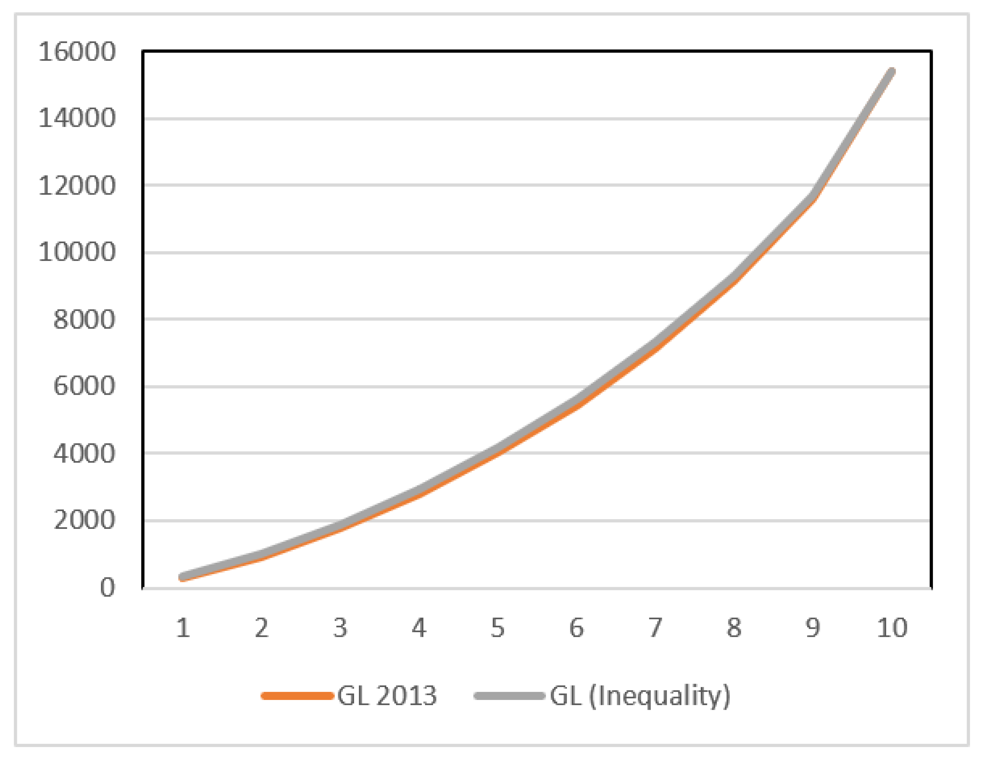
Figure 1 illustrates GL dominance of 2017 over 2013. In addition to the higher GL welfare, Spanish economic growth was weakly pro-poor. Eight positive and significant deciles (1–8) and no negative and significant deciles result in a weakly pro-poor ranking. In other words, if one only considers the effect of economic inequality, welfare associated with income distribution grew. Therefore, growth in Spain between 2013 and 2017 was pro-poor. Figure 2 illustrates the pro-poor dominance of 2017 over 2013.
The overall result for Spain is that economic growth between 2013 and 2017 can be classified as weekly pro-poor. However, an additional question naturally arises: Is this trend common to all Spanish regions? This question is especially important as the behavior of large regions may strongly affect the evolution of the country as a whole. Appendix A provides the GL dominance and pro-poor dominance results for each of the 17 Spanish regions. These results are summarized in Table 3.
Table 3 shows there is a group of regions in which 2017 GL strongly dominates 2013: Andalusia, Aragon, Asturias, Balearic Islands, Castile-Leon, Catalonia, Extremadura, and Murcia. In the Canary Islands, Cantabria, Castile La Mancha, Community of Valencia, Galicia, and la Rioja, 2017 GL weakly dominates 2013. For Madrid and the Basque Country, we find no statistical difference in the 2013 and 2017 GL curves.
Turning to regional pro-poor dominance, we find that growth was weakly pro-poor in seven of Spain’s 17 regions. In nine regions, growth was neither pro-poor nor anti-poor. Only in Cantabria can we conclude that growth was weakly anti-poor. This implies that in most parts of Spain, the increase in well-being was mainly due to the rise in GDP, while the change in inequality and poverty played a minor role.

5. Discussion and Conclusions

In this paper, we present and apply, for the first time in this context, a statistical test to analyze the pro-poorness nature of economic growth in Spain and its regions. The main novelty of this technique, in addition to those inherent to stochastic dominance, is the possibility of introducing statistical inference into the analysis, which leads to more accurate results by avoiding sampling error problems. This implies that the pro-poorness nature of economic growth can be measured with a greater degree of reliability.
From the empirical point of view, the conclusions to emerge from our research questions are as follows. In relation to the first question concerning whether or not economic growth was pro-poor in Spain and its regions between 2013 and 2017, we can conclude that economic growth in Spain as a whole was weakly pro-poor. As for the regional effects of growth, we find that in seven of Spain’s 17 regions growth was weakly pro-poor, in nine regions growth was neither pro-poor nor anti-poor and that only in one region was growth weakly anti-poor. Regarding the second research question concerning whether or not there were disparities in the impact of growth on poverty across regions, the empirical evidence shows that the “pro-poorness” nature of growth was unequal across regions, due to the different trends in inequality.
Therefore, we can conclude that the phase of economic growth which has followed the Great Recession in Spain has been characterized, as expected, by an increase in well-being, not only in the country as a whole but also in each of its regions. This conclusion can be deduced from the generalized Lorenz curve comparisons, which consider efficiency and equity criteria, and which show a strong dominance of the 2017 curves over those of 2013. However, the main source of the increase in well-being has been the rise in average income. The inequality effect has not been intense enough to generate strong pro-poor growth in all Spanish regions. The case of Cantabria is especially interesting, as in this region economic growth has, in fact, been anti-poor. Thus, in line with other analyses, during the economic recovery phase, the lower tail of income distribution does not appear to have fully recovered from the profound effects of the economic crisis that increased polarization in Spanish society. In other words, economic growth by itself does not seem sufficient to compensate the poorer for the losses they suffered during the crisis, such that more redistributive efforts are needed if the increase in GDP is to reach society as a whole.

Author Contributions

Conceptualization, methodology, formal analysis, investigation, resources, writing, visualization, supervision, funding acquisition, I.A., C.-G.P. and M.P.-A.; data, software, validation, C.G.-P. and M.P.-A. All authors have read and agreed to the published version of the manuscript.

Funding

This research was funded by the Spanish Ministry of Economy and Competitiveness (Project ECO2016-77900-P), by the Consejería de Educación, Cultura y Deportes de Castilla-La Mancha (Project SBPLY/19/180501/000132) and by the Comunidad de Madrid (Project H2019/HUM-5793-OPINBI).

Acknowledgments

The financial support provided by the Spanish Ministry of Economy and Competitiveness (Project ECO2016-77900-P), by the Consejería de Educación, Cultura y Deportes de Castilla-La Mancha (Project SBPLY/19/180501/000132) and by the Comunidad de Madrid (Project H2019/HUM-5793-OPINBI) is acknowledged.

Conflicts of Interest

The authors declare no conflict of interest.

Appendix A

Detailed Tables (2013−2017)
Table A1. Andalusia.
Decile G ^ L 1 G ^ L 2 T G L i G ^ L I T G L i
1217.87295.31−4.93***262.432.52-
2720.08898.43−5.84***795.672.23-
31398.041691.55−7.27***1494.032.18-
42212.682592.44−7.57***2289.711.43-
53157.303645.91−7.75***3214.640.86-
64282.054872.42−7.63***4302.270.25-
75557.716308.95−8.09***5553.03−0.05-
87084.438004.59−8.05***7047.49−0.32-
99003.5510184.25−8.11***8968.17−0.24-
1012118.2213757.36−7.64***12118.220.00-
Note: (***): Statistically significant at the 1-percent level. (**): Statistically significant at the 5-percent level. (*): Statistically significant at the 10-percent level.
Table A2. Aragon.
Table A2. Aragon.
Decile G ^ L 1 G ^ L 2 T G L i G ^ L I T G L i
1424.76570.67−3.66***589.323.48***
21172.911453.63−4.51***1480.754.36***
32176.552575.67−4.48***2631.494.68***
43362.063914.62−4.67***3949.914.69***
54852.945362.81−3.43***5437.163.80***
66605.377102.28−2.73*7229.383.37***
78504.559154.04−2.97**9216.843.23**
810741.5811245.83−2.02-11397.472.62*
913435.4913830.47−1.30-14047.382.01-
1017662.0117393.280.68-17662.010.00-
Note: (***): Statistically significant at the 1-percent level. (**): Statistically significant at the 5-percent level. (*): Statistically significant at the 10-percent level.
Table A3. Asturias.
Table A3. Asturias.
Decile G ^ L 1 G ^ L 2 T G L i G ^ L I T G L i
1290.73428.34−3.05**400.952.08-
21039.151351.00−4.03***1241.182.26-
31987.522436.68−4.63***2271.082.56*
43107.883735.53−4.97***3450.952.44-
54448.565214.94−4.85***4831.672.22-
66022.996892.35−4.63***6384.001.79-
77892.868937.05−4.61***8213.981.33-
89967.0711,076.18−4.30***10,218.330.93-
912,453.6213,689.74−4.05***12,659.670.66-
1016,011.2117,343.44−3.49***16,011.210.00-
Note: (***): Statistically significant at the 1-percent level. (**): Statistically significant at the 5-percent level. (*): Statistically significant at the 10-percent level.
Table A4. Balearic Islands.
Decile G ^ L 1 G ^ L 2 T G L i G ^ L I T G L i
1138.20591.29−9.45***521.584.63***
2768.001468.03−7.73***1239.373.76***
31690.522515.57−7.28***2091.422.70*
42796.393896.65−7.28***3186.302.07-
54185.515441.83−6.58***4486.171.32-
65620.297166.91−7.03***5869.350.98-
77371.889161.80−6.64***7487.480.38-
89575.5511,972.56−7.20***9618.210.12-
912,074.8114,459.51−6.29***11,737.38−0.85-
1015,729.0619,246.54−6.23***15,729.060.00-
Note: (***): Statistically significant at the 1-percent level. (**): Statistically significant at the 5-percent level. (*): Statistically significant at the 10-percent level.
Table A5. Canary Islands.
Decile G ^ L 1 G ^ L 2 T G L i G ^ L I T G L i
1133.96219.70−2.02-211.201.56-
2664.66821.10−2.57*764.851.49-
31388.751516.73−1.44-1422.960.36-
42305.032443.10−1.29-2288.52−0.15-
53358.473521.91−1.25-3301.88−0.42-
64587.724807.72−1.41-4503.00−0.53-
75978.116326.41−1.85-5909.47−0.36-
87637.618136.33−2.24-7618.08−0.09-
99723.1410,391.65−2.50-9702.60−0.08-
1012,504.5213,332.92−2.47-12,504.520.00-
Note: (***): Statistically significant at the 1-percent level. (**): Statistically significant at the 5-percent level. (*): Statistically significant at the 10-percent level.
Table A6. Cantabria.
Decile G ^ L 1 G ^ L 2 T G L i G ^ L I T G L i
1449.46413.291.20-359.31−2.98**
21126.841163.57−0.59-1006.54−1.72-
32055.352223.19−1.72-1941.44−1.00-
43221.853392.67−1.33-3060.59−1.09-
54329.164758.48−2.78*4181.95−0.83-
65708.756281.81−3.04**5505.29−0.95-
77251.638112.03−3.91***7083.63−0.67-
89055.1410,133.63−4.12***8892.78−0.56-
911,220.6712,590.74−4.50***11,069.07−0.46-
1014,137.2516,142.01−4.91***14,137.250.00-
Note: (***): Statistically significant at the 1-percent level. (**): Statistically significant at the 5-percent level. (*): Statistically significant at the 10-percent level.
Table A7. Castile−Leon.
Decile G ^ L 1 G ^ L 2 T G L i G ^ L I T G L i
1293.33497.40−6.98***449.093.99***
2966.481339.93−7.63***1201.393.88***
31841.662371.35−7.99***2120.353.54***
42888.333601.80−8.05***3212.923.19**
54156.705026.49−7.68***4475.812.54-
65624.726622.83−7.36***5885.251.76-
77347.918472.60−6.92***7548.141.16-
89308.4910599.77−6.77***9436.670.64-
911,598.0213,221.47−7.17***11,712.020.49-
1015,080.3116,992.43−6.17***15,080.310.00-
Note: (***): Statistically significant at the 1-percent level. (**): Statistically significant at the 5-percent level. (*): Statistically significant at the 10-percent level.
Table A8. Castile−La Mancha.
Decile G ^ L 1 G ^ L 2 T G L i G ^ L I T G L i
1255.36274.17−0.57-244.20−0.34-
2883.94887.76−0.07-822.68−1.11-
31593.501689.15−1.33-1524.12−0.92-
42497.602680.24−1.95-2414.92−0.83-
53489.953875.82−3.38***3460.60−0.24-
64725.025200.53−3.41***4672.70−0.36-
76090.616746.68−4.08***6053.25−0.22-
87707.278529.88−4.24***7628.80−0.39-
99828.6110,697.27−3.70***9603.13−0.94-
1012,823.5414,304.71−4.13***12,823.540.00-
Note: (***): Statistically significant at the 1-percent level. (**): Statistically significant at the 5-percent level. (*): Statistically significant at the 10-percent level.
Table A9. Catalonia.
Decile G ^ L 1 G ^ L 2 T G L i G ^ L I T G L i
1329.92504.38−7.90***475.694.66***
21097.891408.84−7.65***1319.044.16***
32158.252582.20−7.24***2402.953.29***
43441.934008.95−7.58***3731.903.07**
54941.215668.03−7.72***5286.322.98**
66688.067580.21−7.99***7060.582.77*
78704.419791.26−8.21***9067.392.33-
811,038.9312,142.25−7.28***11,294.301.44-
913,809.6215,083.14−6.99***14,025.511.03-
1018,104.2519,479.44−5.63***18,104.250.00-
Note: (***): Statistically significant at the 1-percent level. (**): Statistically significant at the 5-percent level. (*): Statistically significant at the 10-percent level.
Table A10. Community of Valencia.
Decile G ^ L 1 G ^ L 2 T G L i G ^ L I T G L i
1322.52351.78−1.02-320.83−0.06-
2936.311037.21−2.39-939.690.08-
31708.791883.21−3.04**1708.93−0.00-
42641.492928.78−3.76***2660.440.24-
53726.314206.10−4.89***3808.730.81-
64998.715626.07−5.33***5123.191.03-
76430.757251.26−6.04***6594.251.18-
88109.969143.24−6.20***8312.811.21-
910,219.6011,414.70−5.98***10,378.060.80-
1013,445.5914,800.70−4.97***13,445.590.00-
Note: (***): Statistically significant at the 1-percent level. (**): Statistically significant at the 5-percent level. (*): Statistically significant at the 10-percent level.
Table A11. Extremadura.
Decile G ^ L 1 G ^ L 2 T G L i G ^ L I T G L i
1256.32418.92−5.88***377.293.35***
2781.881056.61−6.08***963.343.33***
31465.591798.09−5.60***1659.472.85**
42282.202612.81−4.54***2438.651.95-
53225.243560.25−3.76***3328.461.07-
64282.204683.38−3.61***4353.780.61-
75534.165943.70−3.04**5544.490.07-
87026.687479.64−2.73*6946.05−0.47-
98744.869287.29−2.65*8631.91−0.55-
1011,344.6912,180.81−3.01**11,344.690.00-
Note: (***): Statistically significant at the 1-percent level. (**): Statistically significant at the 5-percent level. (*): Statistically significant at the 10-percent level.
Table A12. Galicia.
Table A12. Galicia.
Decile G ^ L 1 G ^ L 2 T G L i G ^ L I T G L i
1435.57420.030.50-393.85−1.28-
21187.151211.59−0.49-1103.32−1.65-
32133.782251.99−1.81-2043.23−1.35-
43217.283426.72−2.45-3123.88−1.06-
54455.404846.61−3.70***4403.97−0.47-
65892.266425.76−4.15***5867.56−0.19-
77502.428270.83−5.07***7530.010.18-
89412.0210,374.55−5.33***9451.740.22-
911,688.2712,940.61−5.69***11,790.830.47-
1015,273.4016,757.58−4.90***15,273.400.00-
Note: (***): Statistically significant at the 1-percent level. (**): Statistically significant at the 5-percent level. (*): Statistically significant at the 10-percent level.
Table A13. Madrid.
Table A13. Madrid.
Decile G ^ L 1 G ^ L 2 T G L i G ^ L I T G L i
1354.03380.31−0.86-370.870.53-
21151.801251.39−2.01-1200.830.95-
32208.992339.78−1.86-2274.500.90-
43498.263712.54−2.33-3603.621.11-
55032.215270.14−2.12-5117.870.74-
66846.647055.83−1.53-6862.970.12-
78901.929163.87−1.59-8897.92−0.02-
811,333.7111,661.77−1.69-11,323.14−0.05-
914,257.7214,636.98−1.64-14,226.18−0.13-
1018,789.3319,338.41−1.67-18,789.330.00-
Note: (***): Statistically significant at the 1-percent level. (**): Statistically significant at the 5-percent level. (*): Statistically significant at the 10-percent level.
Table A14. Murcia.
Table A14. Murcia.
Decile G ^ L 1 G ^ L 2 T G L i G ^ L I T G L i
1251.58348.16−4.03***288.671.28-
2796.44936.83−3.13**793.10−0.07-
31459.971727.14−4.25***1459.79−0.00-
42239.902696.13−5.36***2292.010.54-
53185.983905.49−6.69***3302.270.96-
64268.885194.65−7.09***4419.611.04-
75513.756734.35−7.81***5733.271.29-
86992.168512.52−8.15***7248.691.30-
98796.5710,740.38−8.49***9115.901.36-
1011,714.8213,819.90−6.88***11,714.820.00-
Note: (***): Statistically significant at the 1-percent level. (**): Statistically significant at the 5-percent level. (*): Statistically significant at the 10-percent level.
Table A15. Navarre.
Table A15. Navarre.
Decile G ^ L 1 G ^ L 2 T G L i G ^ L I T G L i
1558.78629.74−1.41-639.611.54-
21475.691774.31−3.01**1743.912.56*
32732.863158.35−3.11**3144.892.90**
44255.664762.26−3.07**4729.052.79*
55972.106531.70−2.84**6460.842.44-
67888.498524.36−2.71*8427.182.28-
710,203.6710,741.42−2.01-10,641.051.64-
812,677.1313,206.97−1.74-13,039.451.19-
915,616.1815,881.73−0.77-15,727.530.32-
1019,549.8719,777.17−0.52-19,549.870.00-
Note: (***): Statistically significant at the 1-percent level. (**): Statistically significant at the 5-percent level. (*): Statistically significant at the 10-percent level.
Table A16. La Rioja.
Decile G ^ L 1 G ^ L 2 T G L i G ^ L I T G L i
1558.78629.74−1.41-639.611.54-
21475.691774.31−3.01**1743.912.56*
32732.863158.35−3.11**3144.892.90**
44255.664762.26−3.07**4729.052.79*
55972.106531.70−2.84**6460.842.44-
67888.498524.36−2.71*8427.182.28-
710,203.6710,741.42−2.01-10,641.051.64-
812,677.1313,206.97−1.74-13,039.451.19-
915,616.1815,881.73−0.77-15,727.530.32-
1019,549.8719,777.17−0.52-19,549.870.00-
Note: (***): Statistically significant at the 1-percent level. (**): Statistically significant at the 5-percent level. (*): Statistically significant at the 10-percent level.
Table A17. Basque Country.
Decile G ^ L 1 G ^ L 2 T G L i G ^ L I T G L i
1465.98496.74−0.59-489.260.43-
21476.691586.69−1.35-1553.600.91-
32849.442902.83−0.49-2850.720.01-
44438.964487.22−0.35-4395.21−0.31-
56264.516309.48−0.27-6173.36−0.55-
68377.098348.900.14-8199.69−0.90-
710,662.0510,702.33−0.18-10,469.83−0.86-
813,326.4213,397.08−0.27-13,106.31−0.83-
916,511.5016,679.90−0.54-16,331.65−0.57-
1020,956.8221,417.80−1.13-20,956.820.00-
Note: (***): Statistically significant at the 1-percent level. (**): Statistically significant at the 5-percent level. (*): Statistically significant at the 10-percent level.

References

  1. Danziger, S.; Gottschalk, P. Do Rising Tides Lift All Boats? The Impact of Secular and Cyclical Changes on Poverty. Am. Econ. Rev. 1986, 76, 405–410. [Google Scholar]
  2. Datt, G.; Ravallion, M. Growth and redistribution components of changes in poverty measures: A decomposition with applications to Brazil and India. J. Dev. Econ. 1992, 38, 275–295. [Google Scholar] [CrossRef]
  3. Kakwani, N. Statistical Inference in the Measurement of Poverty. Rev. Econ. Stat. 1993, 75, 632–639. [Google Scholar] [CrossRef]
  4. Kakwani, N. On Measuring Growth and Inequality Components of Poverty with Application to Thailand. J. Quant. Econ. 2000, 16, 67–80. [Google Scholar]
  5. Ravallion, M.; Chen, S. Measuring Pro-Poor Growth. Econ. Lett. 2003, 78, 93–99. [Google Scholar] [CrossRef] [Green Version]
  6. Manwa, H.; Manwa, F. Poverty Alleviation through Pro-Poor Tourism: The Role of Botswana Forest Reserves. Sustainability 2014, 6, 5697–5713. [Google Scholar] [CrossRef] [Green Version]
  7. Sun, R.; Mi, J.; Cao, S.; Gong, X. Classifying Livelihood Strategies Adopting the Activity Choice Approach in Rural China. Sustainability 2019, 11, 3019. [Google Scholar] [CrossRef] [Green Version]
  8. Kakwani, N.; Pernía, M. What is Pro-poor Growth? Asian Dev. Rev. 2000, 18, 1–16. [Google Scholar]
  9. Son, H. A note on Pro-Poor Growth. Econ. Lett. 2004, 82, 307–314. [Google Scholar] [CrossRef]
  10. Kakwani, N.; Son, H. Poverty Equivalent Growth Rate. Rev. Income Wealth 2008, 54, 643–655. [Google Scholar] [CrossRef] [Green Version]
  11. Dollar, D.; Kraay, A. Growth is good for the poor. J. Econ. Growth 2002, 7, 195–225. [Google Scholar] [CrossRef]
  12. Adams, J.R.H. Economic growth, inequality and poverty: Estimating the growth elasticity of poverty. World Dev. 2004, 32, 1989–2014. [Google Scholar] [CrossRef]
  13. Balakrishnan, R.; Steinberg, C.; Syed, M.M.H. The Elusive Quest for Inclusive Growth: Growth, Poverty, and Inequality in Asia; IMF Working Paper (No. WP/13/152); IMF: Washington, DC, USA, 2013; pp. 1–35. [Google Scholar]
  14. Janvry, A.D.; Sadoulet, E. Agricultural growth and poverty reduction: Additional evidence. World Bank Res. Obs. 2009, 25, 1–20. [Google Scholar] [CrossRef]
  15. Kakwani, N. Growth and poverty reduction: An empirical analysis. Asian Dev. Rev. 2000, 18, 74–84. [Google Scholar]
  16. Ravallion, M. Growth and poverty: Evidence for developing countries in the 1980s. Econ. Lett. 1995, 48, 411–417. [Google Scholar] [CrossRef]
  17. Rodrik, D. Growth versus poverty reduction: A hollow debate. Financ. Dev. 2000, 37, 8–9. [Google Scholar]
  18. McCulloch, N.; Baulch, B. Assessing the Poverty Bias of Growth Methodology and an Application to Andhra Pradesh and Uttar Pradesh; Working Paper 98; Institute of Development Studies: Brighton, UK, 1999. [Google Scholar]
  19. Son, H.H.; Kakwani, N. Global estimates of pro-poor growth. World Dev. 2008, 36, 1048–1066. [Google Scholar] [CrossRef] [Green Version]
  20. Araar, A.; Duclos, J.Y.; Audet, M.; Makdissi, P. Testing for pro-poorness of growth, with an application to Mexico. Rev. Income Wealth 2009, 55, 853–881. [Google Scholar] [CrossRef]
  21. Duclos, J.; Wodon, Q. What is Pro-Poor. Working Paper 04-25. Centre Interuniversitaire Sur le Risque, les Politiques Économiques et L’emploi; CIRPEE Universite Laval: Quebec, QC, Canada, 2004. [Google Scholar]
  22. Essama-Nssah, B. A Unified Framework for Pro-Poor Growth Analysis; Poverty Reduction Group, the World Bank: Washington, DC, USA, 2004. [Google Scholar]
  23. Warr, P. Pro-Poor Growth, Poverty Research Centre, Division of Economics, Research School of Pacific and Asia Studies; The Australian national University: Camberra, Australia, 2006. [Google Scholar]
  24. Chen, S.; Ravallion, M. China’s (uneven) Progress against Poverty Governing Rapid Growth in China; Routledge: London, UK, 2009. [Google Scholar]
  25. Anyanwu, J.C.; AErhijakpor, E.O. Do international remittances affect poverty in Africa? Afr. Dev. Rev. 2010, 22, 51–91. [Google Scholar] [CrossRef]
  26. Ulriksen, M.S. Questioning the pro-poor agenda: Examining the links between social protection and poverty. Dev. Policy Rev. 2012, 30, 261–281. [Google Scholar] [CrossRef]
  27. Thorbecke, E. The interrelationship linking growth, inequality and poverty in Sub-Saharan Africa. J. Afr. Econ. 2013, 22, 15–48. [Google Scholar] [CrossRef]
  28. Oloyede, B.B. Effect of poverty reduction programmes on economic development evidence from Nigeria. Arab. J. Bus. Manag. Rev. 2014, 4, 26–37. [Google Scholar] [CrossRef]
  29. Bikorimana, G.; Shengmin, S.U.N. Lessons learnt for Rwanda from China’s poverty reduction strategies: Policy analysis review. J. Econ. Bibliogr. 2019, 6, 52–98. [Google Scholar]
  30. Dhongde, S.; Silber, J. On distributional change, pro-poor growth and convergence. J. Econ. Inequal. 2016, 14, 249–267. [Google Scholar] [CrossRef] [Green Version]
  31. Loayza, N.; Raddatz, C. The composition of growth matters for poverty alleviation. J. Dev. Econ. 2010, 93, 137–151. [Google Scholar] [CrossRef] [Green Version]
  32. Montalvo, J.; Ravallion, M. The pattern of growth and poverty reduction in China. J. Comp. Econ. 2010, 38, 2–16. [Google Scholar] [CrossRef]
  33. Ayala, L.; Palacio, J.I. Hogares de Baja Renta en España: Caracterización y Factores de Cambio. Rev. De Econ. Appl. 2000, 23, 35–70. [Google Scholar]
  34. Farré, L.; Vella, F. Macroeconomic Conditions and the Distribution of Income in Spain. Labour 2008, 22, 383–410. [Google Scholar] [CrossRef]
  35. Ayala, L.; Jurado, M. Pro-poor Economic Growth, Inequality and Fiscal Policy: The Case of Spanish Regions. Reg. Stud. 2011, 45, 103–121. [Google Scholar] [CrossRef]
  36. Sotelsek, A.; Bishop, J. Dominance Testing for “Pro-Poor” Growth with an Application to European Growth. Empir. Econ. 2012, 43, 723–739. [Google Scholar] [CrossRef]
  37. Shorrocks, A.F. Ranking income distributions3. Economica 1983, 50, 3–17. [Google Scholar] [CrossRef] [Green Version]
  38. Atkinson, A.B. On the Measurement of Poverty. Econometrica 1987, 55, 749–764. [Google Scholar] [CrossRef]
  39. Bishop, A.J.; Formby, J.P.; Thistle, P.D. Statistical Inference, Income Distributions and Social Welfare, in Research on Economic Inequality; Slotje, D.J., Ed.; JAI Press: Greenwich, CN, USA, 1989. [Google Scholar]
  40. Stoline, M.R.; Ury, H.K. Tables of the Studentized Maximum Modulus Distributions and an application to multiple comparisons among means. Technometrics 1979, 21, 87–93. [Google Scholar] [CrossRef]
  41. Beach, C.; Davidson, R. Distribution-Free Statistical Inference with Lorenz Curves and Income Shares. Rev. Econ. Stud. 1983, 50, 723–735. [Google Scholar] [CrossRef]
Figure 1. Spanish generalized Lorenz curve. 2013–2017.
Sustainability 12 01728 g001
Figure 2. Inequality effect Spanish generalized Lorenz curve in 2017.
Sustainability 12 01728 g002
Table 1. Unemployment rate, poverty rates and average incomes (2013–2017) in Spain and its regions.
Country/RegionsUnemployment Rates %Poverty Rates %Per Capita Income Euros
201320172013201720132017
Spain26.0917.2222.221.510,39111,412
Andalusia36.2225.5133.332.080799258
Aragon21.3911.6516.914.212,03711,990
Asturias24.1313.7116.714.011,25112,085
Balearic Islands22.2612.4317.915.410,66013,240
Canary Islands33.7323.4627.632.183028964
Cantabria20.4413.5620.619.9982411,239
Castile-Leon21.7514.0820.416.110,40611,949
Castile-La Mancha29.9720.7728.429.985459533
Catalonia23.1213.4115.813.612,20513,338
Valencia28.0518.1726.226.0914410,232
Extremadura33.8726.2233.137.677298503
Galicia22.0415.6715.418.810,23511,239
Madrid19.7613.3414.716.112,59713,279
Murcia28.9818.0337.228.677679111
Navarre17.9310.2411.98.913,22113,585
La Rioja16.5812.0016.216.611,12012,029
Basque Country20.0411.3110.28.614,28114,722
Source: Spanish Statistical Office.
Table 2. Generalized Lorenz dominance and pro-poor dominance Spain (2013–2017).
Decile G ^ L 1 G ^ L 2 T G L i G ^ L I T G L i
1281.71369.50−11.55***343.667.05***
2920.701100.60−14.48***1020.927.13***
31768.342042.74−15.81***1890.216.31***
42799.053181.56−16.74***2946.375.87***
54024.124532.24−17.58***4195.585.47***
65459.396098.00−18.12***5642.574.85***
77141.627915.41−18.05***7321.643.97***
89148.3810,047.64−17.49***9291.362.66*
911,609.9212,650.47−16.92***11,690.881.28 -
1015,404.1916,668.74−14.82***15,404.190.00 -
Note: (***): Statistically significant at the 1-percent level. (**): Statistically significant at the 5-percent level. (*): Statistically significant at the 10-percent level.
Table 3. Summary of generalized Lorenz and pro-poor dominance1. 2013–2017.
Country/RegionGL
Dominance
Pro-Poor
Dominance
RegionGL
Dominance
Pro-Poor
Dominance
Spain+w+Catalonia+w+
Andalusia+=C. Valenciaw+=
Aragón+w+Extremadura+w+
Asturias+w+Galiciaw+=
Balearic Islands+w+Madrid==
Canary Islandsw+=Murcia+=
Cantabriaw+w-Navarrew+w+
Castile-Leon+w+La Riojaw+=
Castile-La Manchaw+=Basque Country==
Note: “+” denotes dominance of second year over first or pro-poor dominance, “–” denotes dominance of first year over second or anti-poor dominance, “=” denotes equivalences, and w denotes that dominance is weak.

