Objective Environmental Indicators and Subjective Well-Being: Are They Directly Related?

Abstract

This paper discusses how objective environmental indicators affect the measure of a country’s well-being. The dependent variable in the analysis is subjective well-being (WB), for which the objective environmental variable we use is per capita carbon dioxide (CO₂) emissions. The paper refers to the relationship between subjective well-being and a set of objective variables representing the four basic types of capital to satisfy human needs and to ensure the well-being of future generations based on the ecological economic systems. Implementing different mediation models, estimated using structural equation modeling, we discover that the objective environmental variable does not directly affects the country’s subjective well-being, while, according to different models, the mediated effects are statistically significant in explaining subjective well-being. The surprising results lead us to think that the environmental risks related to CO₂ emissions might not be correctly perceived by the public.

1. Introduction

The idea of well-being as a multidimensional concept is not new (e.g., [1,2]). According to Sen’s “capability approach” [3], individual well-being is based on one’s capabilities, reflecting the combination of interrelated functioning by an individual in various spheres of life. Much more recently, despite differences in approach, most researchers have assessed the multidimensionality of the concept of well-being (see [4,5,6,7]), indeed, without reaching a unanimous view leading to an ideal measure of well-being [8]. However, in their report by the Commission on the Measurement of Economic Performance and Social Progress [9], the Stiglitz-Sen-Fitoussi Commission endorsed the use of a subjective measure of well-being (not isolated from objective measures) to design, monitor, and evaluate social and economic progress.

Multidimensional, objective or subjective measures of well-being are clearly related to Sustainable Developments Goals (SDGs), and in fact they are listed under SDGs 1 and 10—Goal 1 “No poverty” and Goal 10 “Reduced inequalities”, with special focus on Target 1.2: “By 2030, reduce at least by half the proportion of men, women and children of all ages living in poverty in all its dimensions according to national definitions”. These relationships were clearly highlighted in some recent original research [10,11].

Going from basic research to political decisions, governments would like to know how objective variables affect well-being at both the individual and territorial level. To embark on a path toward sustainability, we need to understand the complex connection between well-being and objective variables representing the three basic pillars of sustainability: the environmental, social, and economic dimensions. This classical viewpoint on sustainability inspired many different approaches, such as those based on a large number of juxtaposed indicators to monitor the development of countries, or systems in general (e.g., the Millennium Development Goals indicators [12]; the EU Strategy for Sustainable Development indicators [13]), and also multidimensional indicators to properly capture the multidimensional nature of sustainable development [14] or the simple input-state-output framework (environment–society–economy), successfully applied to investigate economic systems (e.g., the national or the regional economies) regarding their level of sustainability [15] or the one highlighting the interconnection “between built, social, human and natural capital required to produce human well-being” [16]. In a view of sustainability closer to the local context, it is worth remembering the “municipal scorecards”, a governance perspective, acknowledging that good governance is a crucial aspect to enhancing the confidence of citizens and other stakeholders [17] as well as the benefits induced by a proper regulation, for example, concerning quality service and price regulation [18] and also the implications of sustainability and corporate social responsibility on the society [19].

Last but not least, there is the individual perception. It is known that individuals might perceive the connection between their well-being and objective variables, representing sustainability dimensions, inaccurately. These misleading perceptions may be due to many factors: personal point of view, lack of information, poor capacity for elaboration, misleading picture provided by the media, cultural factors, etc.

In the view of understanding the complex connection between well-being and objective variables, the paper considers the relationship between subjective well-being and a set of objective variables representing the four basic types of capital to satisfy human needs and to ensure the well-being of future generations based on the ecological economic system [20], and as a novelty we aim to understand how a factor of environmental stress, like air pollution, affects a country’s well-being.

We conduct the analysis at the country level by specifying mediation models estimated with a structural equation model approach. The results show that the direct effect of per capita CO₂ emissions does not have a significant direct effect on a country’s well-being.

The remainder of this work is organized as follows. The motivation of the paper and the background are given in Section 2. The dataset and variables used in the empirical analysis are described in Section 3, which also describes the data and the modelling strategy. In Section 4, the main results are provided. Finally, Section 5 concludes the paper, and also evidences the limitations.

2. Motivation and Background

The core of the model of the ecological economic system, introduced in [20], is the four basic types of capital, represented in the model by objective variables: natural, human, social, and built capital. A balance among them is a necessary condition for satisfying human needs and ensuring the well-being of future generations. A country-level analysis in [6] showed that the Human Development Index (HDI) explains a significant proportion of subjective well-being; however, natural capital also has a significant, positive impact on well-being.

Given these findings, it is questionable whether environmental degradation has an adverse impact on human well-being. Evidence on this negative impact can be found in [21], whereas previous results state that pressure on the environment, such as that caused by energy consumption, does not necessarily have a negative impact on human well-being [22].

This background gives rise to a new research question: “how can environmental stress contribute to human well-being?” This question was first posed in the literature on structural human ecology (see [23,24]), a research area that aims to understand all aspects of the relationship between people and the environment. In this paper, the previous general research question is taken into account, and we wonder more specifically: “how does environmental stress, meaning the impact of air pollution, affect a country’s well-being?”. The investigation is limited to a country-level analysis, considering subjective well-being (WB) as a measure of human well-being (the model dependent variable), and a series of objective indicators as model predictors. The choice of using only objective measures as dependent variables (predictors) is related to the idea that policies are geared toward objectives, generally measured by observable and quantitative factors.

3. Materials and Methods

3.1. Data

The concept of well-being is widely used; however, no commonly agreed definition of it exists. Indeed, the terms “well-being,” “quality of life,” “happiness,” and “life satisfaction” are used interchangeably. In this paper, we used data on experienced well-being (WB) drawn from responses to the ladder of life question, collected in the 2012 Gallup World Poll. The survey was designed to measure dimensions of overall well-being for individuals age 15 and over, in order to obtain a WB evaluation at the country level. To compute the WB score, Gallup weights the responses to correct for unequal selection probability and nonresponses and to match the demographics in each country. The WB score is calculated using a ten-point Likert scale, in which 10 means the best possible life and 0 means the worst possible life. In the analysis, the point scale is considered a cardinal measure, regarding the empirical results, stating that treating happiness scores as cardinal data does not have appreciable effects on the empirical results (see [25,26]).

We use CO₂ emissions as the objective environmental variable, with data from 2014 (the latest data available) from the World Bank’s World Development Indicators. The variable used in the analysis is per capita CO₂ (CO₂_pc in metric tons). CO₂ is commonly known as a greenhouse gas that is emitted by cars and other fossil-fuel-burning entities. The increasing concentration of CO₂ is the primary contributor to rising global temperatures. Aside from the environmental dangers, CO₂ emissions are also considered responsible for some health risks. Human and built capital are represented together in the analysis, as the UN’s Human Development Index (HDI). The HDI is a composite index, made up of an education index, a standard of living index, and a longevity index. Each single index is normalized, so as to obtain the HDI, which ranges from 0 to 1. Details on the computation of the HDI are available in the Human Development Report (2015; see Technical Notes).

As regards the social capital variable, we use the yearly Democracy Index, which provides a picture of the state of democracy worldwide in 165 independent states. The Economist Intelligence Unit’s Democracy Index is based on five categories: electoral process and pluralism, civil liberties, the functioning of government, political participation, and political culture. A three-point scoring system for sixty variables grouped in the five categories mentioned earlier is used. The category indexes are based on the sum of the scores in each category, converted to a scale from 0 to 10. The overall index is computed as the simple average of the five category indexes, using a similar scale.

3.2. Methods

The proposed research question aimed at discovering the underlying mechanism producing a relation between experienced well-being (WB) and an environmental stress factor like per capita CO₂, thus the paper’s research question concerned issues of mediation. Indeed, mediation modeling goes beyond simple cause and effect relationships in an attempt to understand what underlying mechanisms led to the outcome variable. Assuming linear associations between experienced well-being (WB) and natural, human, social, and built capital (see [6,20]) as well as that human and built capital (like HDI) can linearly mediate the effect of the environmental stress factor on WB seems to be reasonable to adopt mediation modeling. The starting point is the simple mediation framework [27]. The model is illustrated in Figure 1. According to this framework, a mediating variable helps to explain how or why an independent variable influences an outcome variable.

The general mediation model requires two equations to estimate the indirect effect of independent variable X on Y: in Equation (1), the mediating variable M is specified as a linear function of X; in Equation (2), the dependent variable Y is specified as a linear function of X and M.

M = i_M+a₁X+e_M,

(1)

Y = i_Y+c’X+bM+e_Y.

(2)

Following the original approach, coefficients of each covariate in the equations can be estimated separately using the regression technique (if equation errors are not correlated). The strong assumption and the drawback of the original mediation framework based on the regression technique compared to a structural equation model (SEM) demonstrated in [28], led us to adopt a SEM strategy to estimate the unknown parameters and the paths. The advantage of SEM over regression models is that estimating all paths simultaneously is more efficient, and thus the SEM framework leads to lower estimated standard errors than regression analysis. A further advantage of the SEM is that it can also facilitate mediation analysis in the case of models relating to measurement errors (also latent variables). Moreover, SEM can be used when a mediation process is extended to multiple independent variables, mediators, or outcomes, whereas, when standard regression is used, ad hoc methods must be adopted to obtain inferences about indirect and total effects.

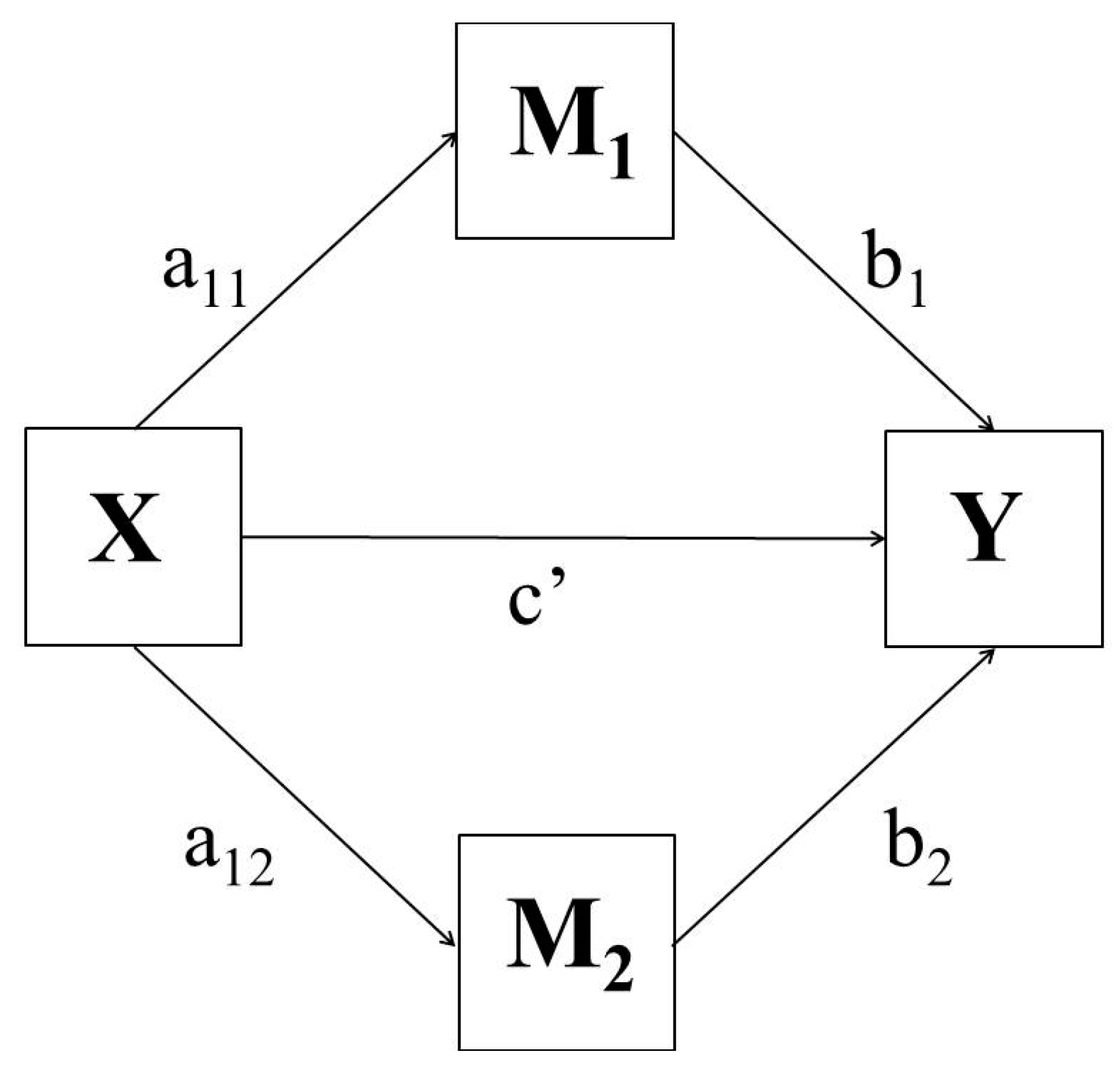
Accordingly, Iacobucci, D. and Zhao, X. [28,29] proposed conducting mediation analysis via SEM by simultaneously estimating the coefficients a₁, b, and c’ and how to evaluate the type of mediation. Specifically, mediation can be divided into the following types:

• complementary mediation, in which the indirect effect (a₁b) and direct effect (c’) both exist and point in the same direction;
• competitive mediation, in which the indirect effect (a1b) and direct effect (c’) both exist and point in opposite directions;
• indirect-only mediation (full mediation), in which the indirect effect (a1b) exists, but not a direct effect;
• direct-only non-mediation, in which a direct effect (c’) exists, but not an indirect effect;
• no-effect non-mediation, in which neither direct nor indirect effects exist.

Beginning with the general mediation model, we explored some possible paths in the analysis. It is possible to hypothesize a structure with more than one mediator, and in this case a multiple mediation model has to be estimated. In our case study, we specified a structure with two parallel mediating variables: M₁ and M₂ (see Figure 2).

The structure requires three equations to estimate the indirect effect of the independent variable X on Y: two equations for the mediating variables and one equation for the dependent variable.

M₁ = i_M1+a₁₁X+e_M1,

(3)

M₂ = i_M2+a₁₂X+e_M2,

(4)

Y = i_Y+c’X+b₁M₁+b₂M₂ +e_Y.

(5)

The parameters of the equation system have been estimated using SEM. The specific indirect effects of X on Y through M₁ and M₂ are, respectively, a₁₁b₁ and a₁₂b₂.

Traditionally, a parametric Sobel test [30] is used to test the significance of the indirect effect of a mediation model. However, the parametric assumption of normality in the Sobel test is not appropriate for testing an indirect effect, that is, a product parameter, and is known to be highly skewed [31]. A bootstrap test can be used [28,32,33] to test whether the influence of an independent variable on a dependent one involves a mediating variable. This test solves that problem by generating an empirical sample distribution of the product parameters. In our empirical analysis, the direct and indirect paths are simultaneously fitted by using SEM, then the bootstrap standard error have been estimated and the bootstrap confidence interval for indirect effects have been computed to obtain the inferential conclusion. More specifically, according to the confidence interval approach, a significant indirect effect is assumed to exist (see [34,35]) if the bootstrap confidence interval does not include zero. Then, it has been shown [36] that a bias-corrected bootstrap confidence interval is the best for detecting a mediating effect when it is present. In addition to assessment of the significance of the mediating effects, it is also interesting to evaluate the strength of the mediation, which is calculated as the ratio of the total indirect effects (a₁₁b₁+a₁₂b₂) to the total effects.

3.3. Analysis

In this section, we specify the variables introduced in the models and their roles.

To address the research question “how does environmental stress, meaning the impact of air pollution, affect a country’s well-being?” in what follows, the dependent variable Y (the endogenous variable according to the SEM framework) was WB, treated as cardinal measure.

In the model of the ecological economic system, introduced in [6,12], the dependent variables included in the model to explain a country’s WB are natural capital, social, built, and human capital. As explained in Section 2, instead of using natural capital, we added an independent variable (the exogenous variable according to the SEM framework) to the model, for environmental degradation, such as CO₂_pc. HDI (an endogenous variable according to SEM) acts as a mediator, assuming that CO₂_pc has an impact on WB through HDI. Finally, the Democracy Index (Dem_Ind), representing social capital, is an exogenous variable.

We conducted the analysis, for all the countries for which the indicators involved in the analysis are not missing, separately for developed countries (DCs, which make up 33% of the countries with higher HDI, or those with HDI > 0.8) and less developed countries (LDCs), following a common approach in environmental social research.

The developed countries consist of Argentina, Australia, Austria, Belarus, Belgium, Bulgaria, Canada, Chile, Croatia, Cyprus, Czech Republic, Denmark, Estonia, France, Germany, Greece, Hungary, Iceland, Ireland, Israel, Italy, Japan, Latvia, Lithuania, Luxembourg, Malta, Montenegro, Netherlands, New Zealand, Norway, Oman, Poland, Portugal, Romania, Slovakia, Slovenia, Spain, Sweden, Switzerland, the United Kingdom, the United States, and Uruguay. The LDCs are Afghanistan, Albania, Algeria, Armenia, Azerbaijan, Benin, Bhutan, Bolivia, Botswana, Brazil, Burkina Faso, Burundi, Cambodia, Chad, China, Colombia, Comoros, Costa Rica, Djibouti, Dominican Republic, Ecuador, Egypt, El Salvador, Ethiopia, Gabon, Georgia, Ghana, Guatemala, Haiti, Honduras, India, Indonesia, Iran, Iraq, Jamaica, Kazakhstan, Kenya, Lebanon, Lesotho, Liberia, Macedonia, Malawi, Malaysia, Mauritania, Mauritius, Mexico, Morocco, Mozambique, Myanmar, Namibia, Nepal, Nicaragua, Niger, Nigeria, Pakistan, Panama, Paraguay, Peru, the Philippines, Rwanda, Senegal, Serbia, Sierra Leone, South Africa, Sri Lanka, Suriname, Tajikistan, Tanzania, Thailand, Timor-Leste, Togo, Tunisia, Turkey, Turkmenistan, Uganda, Ukraine, Uruguay, Uzbekistan, Venezuela, Vietnam, Yemen, Zambia, and Zimbabwe.

Following the SEM approach, we use the ‘sem package’ and the ‘medsem package’ [37] (using Stata 15) to test for mediation.

4. Results

This section describes the results obtained, following two different paths, which were used to answer the general research question “how does environmental stress, meaning the impact of air pollution, affect a country’s well-being?” For the sake of clarity, we reiterate that the reference model of the empirical analysis is the ecological economic system, introduced in [20], and that, in the model specification to predict WB, instead of natural capita, we introduce an environmental factor, like air pollution, in accordance with the literature on structural human ecology.

The data involved in the analysis are from international statistical data sources (introduced in Section 3.1). Summary statistics, for developed countries (DCs) and less developed countries (LDCs), are presented in

Table 1. Summary statistics for the variables involved in models.

	Variable	Mean	Std. Dev.	Min	Max
DCs	WB	6.39	0.91	4.20	7.80
	CO2_pc	7.37	3.93	1.97	17.36
	HDI2015	0.88	0.04	0.80	0.95
	GDP_pc2015	32297.24	22112.87	5949.10	101446.80
	LE	79.05	3.15	70.87	82.24
	Dem_Ind	7.85	1.33	3.04	9.93
	N = 42
LDs	WB	4.97	0.93	2.87	7.30
	CO2_pc	2.22	2.68	0.04	14.36
	HDI2015	0.64	0.12	0.35	0.80
	GDP_pc2015	3829.18	3401.97	300.68	15524.84
	LE	67.39	7.57	48.95	79.08
	Dem_Ind	5.12	1.71	1.50	8.29
	N = 82

, for all variables involved in the models.

4.1. A Single Mediation Model

According to the structure illustrated in Figure 1, Equations (1) and (2) were estimated using the SEM approach to test whether the effect of CO₂_pc on WB is mediated by HDI (HDI2015).

Before considering the direct and indirect effects, let us consider the effect of the control variable Dem_Ind: either for developed and less developed countries, the coefficient of the democracy index is not statistically significant.

The direct effect of CO₂_pc on WB is nearly zero and not statistically significant (see

Table 2. Structural equation model (SEM) model for Equations (1) and (2): estimated coefficients (with standard errors) and significance level.

Structural	DCs		LDCs
(Equation (1)) M = HDI2015
CO2_pc	0.004	***	0.028	***
	(0.002)		(0.008)
_cons	0.846	***	0.574	***
	(0.013)		(0.017)
(Equation (2)) Y = WB
HDI2015	17.104	***	3.521	***
	(3.587)		(0.882)
CO2_pc	0.006		0.029
	(0.027)		(0.034)
Dem_Ind	−0.076		0.095
	(0.111)		(0.063)
_cons	−8.081	***	2.201	***
	(2.416)		(0.420)
N	42		83
CFI	0.498		0.714
SRMR	0.281		0.136

DCs = developed countries; LDCs = less developed countries. * p < 0,05, ** p < 0,01, *** p < 0,001.

, panel (Equation (2)) Y = WB) in both developed and less developed countries. The direct effect of CO₂_pc on WB was also tested, computing the bootstrap confidence intervals. Observing

Table 3. Direct effect, indirect effect, and their relative 95% confidence intervals (bias corrected).

Countries	Direct Effect	95% C.I.	Indirect Effect	95% C.I.
DCs	0.006	[−0.045; 0.056]	0.076	[0.015; 0.137]
LDCs	0.029	[−0.049; 0.108]	0.098	[0.024; 0.172]

, it can be stated that the direct effect is not significant in both the estimated models, for LDCs and DCs, since zero is included in the 95% confidence interval (bias corrected).

We tested the effect of the indirect effects of CO₂_pc on WB through HDI2015, computing the bootstrap confidence intervals. In Table 3, the indirect effect is significant in the two estimated models, since zero is not included in the 95% confidence interval (bias corrected). Specifically, in the specified models, the effect of CO₂_pc on WB is fully mediated by HDI2015. The mediated portion, defined as the ratio of the indirect to the total effect, determines the extent to which the mediation process explains the variance in the dependent variable. In our analysis, the ratio is very large in both cases, particularly in developed countries, HDI2015 explains 93% of the variation in WB, with an indirect effect that is more than thirteen times that of the direct one, and in less developed countries the corresponding figure is 77%.

Regarding the model fitting, we presented the Comparative Fit Index (CFI, normed to the 0–1 range) which compares the fit of the estimated model to the fit of a null model and the Standardized Root Mean Square Residual (SRMR), which is the square root of the difference between the residuals of the sample covariance matrix and the hypothesized model. Both these indexes perform better than the others in estimating the model fit, even in small samples [38,39,40].

In conclusion, in regard to the simple mediation framework, we can state that air pollution, measured as per capita CO₂, does not have a significant direct effect on national wellbeing; the effect of per capita CO₂ on WB is mediated by the Human Development Index.

4.2. Multiple Mediation Model

In the previous analysis, HDI mediates the relationship between CO₂_pc and WB. As HDI is a composite index, calculated by taking the simple average of the life expectancy (LE), standard of living (real GDP per capita, here GDP_pc2015), and educational attainments indexes (which in turn includes the adult literacy rate and gross enrollment ratio), we verified whether the variables that make up HDI have different effects as mediators in the relationship between CO₂_pc and WB. The check was performed with only two mediating variables in order to avoid excessive model complexity. Specifically, the variables included as mediators are LE and GDP_pc2015: LE, because according to recent research [38], at the individual level, health status has an important mediating effect on an objective environmental indicator, and GDP_pc2015, because it is a specific metric that has prevailed since World War II, and it is one of the most renowned factors driving SWB.

A multiple mediation model (see Figure 2) has been specified, with mediators M1 and M2 respectively, GDP_pc2015, and LE. The parameters in Equations (3), (4), and (5) were estimated by the SEM approach. In

Table 4. SEM model for Equations (3), (4), and (5): estimated coefficients. (with standard errors) and significance level.

Structural	DCs		LDCs
(Equation (3)) M1 = GDP_pc2015
CO2_pc	2334.376	**	729.720	***
	(770.587)		(114.928)
_cons	14503.730	**	2206.967	***
	(6497.325)		(398.425)
(Equation (4)) M2 = LE
CO2_pc	0.101		0.961	***
	(0.131)		(0.294)
_cons	78.107	***	65.257	***
	(1.102)		(1.019)
(Equation (5)) Y = WB
GDP_pc2015	0.0000254	***	0.00012	***
	(6.52 × 10−6)		(0.00004)
LE	0.0760		0.025	***
	(0.040)		(0.013)
CO2_pc	0.007		0.00024
	(0.027)		(0.038)
Dem_Ind	−0.048		0.062
	(0.100)		(0.053)
_cons	−0.086		2.472	**
	(2.783)		(0.837)
N	44		82
CFI	0.4268		0.698
SRMR	0.2901		0.139

DCs = developed countries; LDCs = less developed countries. * p < 0,05, ** p < 0,01, *** p < 0,001.

, the direct effect of CO₂_pc on WB is nearly zero and not statistically significant (see Table 4, panel (Equation (5)) in both developed and less developed countries.

As already observed in the simple mediation model, the effect of the control variable Dem_Ind, either for developed and less developed countries, is not statistically significant.

The direct effect of CO₂_pc on WB is nearly zero and not statistically significant (see Table 4, panel (Equation (5)) Y = WB) in both developed and less developed countries. The direct effect of CO₂_pc on WB has also been tested, computing the bootstrap confidence intervals. Observing

Table 5. Direct effect, total indirect effect, specific indirect effect and their relative 95% confidence intervals (bias corrected).

Countries	Direct_Total [95% C.I.]	Ind_Total [95% C.I.]	Ind_GDP [95% C.I.]	Ind_LE [95% C.I.]
DCs	0.007 [−0.014;0.055]	0.067 [0.012;0.121]	0.056 [0.005;0.114]	0.007 [−0.005;0.037]
LDCs	0.0002 [−0.059;0.060]	0.115 [0.033;0.198]	0.104 [0.006;0.199]	0.027 [0.002;0.088]

, it can be stated that the direct effect is not significant in both the estimated models, for LDCs and DCs, since zero is included in the 95% confidence interval (bias corrected). We tested the total indirect effect and the specific mediation effects of GDP_pc2015 and LE on WB, calculating the bootstrap confidence intervals. In Table 5, the total indirect effect is positive and significant in both developed and less developed countries; it accounts for more than 90 percent of the total variation in WB, enabling us to conclude that the effect of CO₂_pc on WB is mediated by the specified mediating variables. As regard to the specific mediation effects, we find that:

• In DCs, the indirect effect of GDP_pc2015 on WB is statistically significant and positive, since the 95% confidence interval does not include zero (see Table 5) whereas the indirect effect of LE on WB is not statistically significant, since zero is included in the 95% confidence interval. So, we conclude that the effect of CO₂_pc on WB is fully mediated by GDP_pc2015.
• In LDCs, total indirect effects are significant and account for more than 99 percent of the total variation in WB (see Table 5), so we conclude that the effect of CO₂_pc on WB is fully mediated by the specified mediating variables; the indirect effects of GDP_pc2015 and LE on WB are both statistically significant (see Table 5). Specifically, the contribution of the indirect effect of GDP_pc2015 to total indirect effects is 79 percent, whereas the remaining 21 percent is due to LE.

5. Discussion and Conclusions

At the outset of the paper, we posed the research question: “how does environmental stress, meaning the impact of air pollution, affect a country’s well-being?” The results presented in the previous section lead to the conclusion that air pollution, measured by CO₂_pc, does not directly affect a country’s well-being. All the estimated models empirically show that the direct effect of CO₂_pc on WB is not statistically significant: the coefficients of CO₂_pc in Equations (2) and (5) (see, respectively, Table 2 and Table 4) are negligible. Specifically, the effect of CO₂_pc is mediated in both the general mediation model and the multiple mediation model.

Indeed, in the general mediation model, where HDI is a mediating variable, the effect of CO₂_pc on WB is fully mediated by HDI2015: in developed countries, HDI2015 explains 93% of the variation in WB, whereas, in LDCs, HDI2015 explains 77% of the WB variability.

In the multiple mediation model, once again, air pollution measured by CO₂_pc does not directly affect a country’s well-being, and CO₂ has a full indirect effect on WB through the mediating variables. Specifically, in LDCs, both the indirect effect of GDP_pc and LE are both significant, even though the weight of the indirect effect of GDP_pc with respect to that of LE is 79% vs 21%. In DCs, the indirect effect of LE is not statistically significant, so the effect of CO₂ on WB is fully mediated by GDP_pc. In their paper dealing directly with the endogeneity of perceived air pollution, controlling for both perceived and actual air pollution, Goetzke and Rave [41] found a similar effect of objective air pollution on WB. Specifically, they found that the increasing of the perceived air pollution is associated with lower happiness, but, using actual pollution as an instrument for perceived pollution, they obtained a not statistically significant but positive coefficient for objective pollution.

Based on the empirical findings, we arrive at a surprising conclusion: a high level of emissions is associated with high GDP per capita, leading to a high level of WB, but CO₂ has no direct effect on WB. Thus, we can answer to the research question proposed at the beginning, stating that our objective indicator of air pollution does not directly affect wellbeing, the effect of CO₂ on WB is fully mediated by the specified mediators.

This relationship and the fact that the increasing concentration of CO₂ is the primary contributor to rising global temperatures demonstrate a conflict between socioeconomic development and reducing carbon emissions. This conflict between economic development and air pollution is a critical matter at the core of international disagreements over addressing climate change. It seems unbelievable that a high concentration of CO₂, recognized as one of the primary contributor to rising global temperatures, does not directly affect societal wellbeing as a severe threat. This finding appears to be similar to the strange general perception of climate change. Indeed, it is unbelievable that a consistent proportion of the USA population does not acknowledge that global warming is happening [42], and that the percentage of Americans that believe that global warming is happening ranges from 43% to 80% at country level.

In regard to climate change, a growing body of scholarship suggests that extreme weather can influence public opinion on climate change ([43,44,45]) and that personal experience with daily weather is more effective than objective statistical information [46]. This finding on the perception of climate change leads us to conclude that perhaps the environmental risks related to environmental degradation are not being perceived correctly at the country level and induces a future research questions: “how does environmental stress, meaning the impact of air pollution, affect local well-being?” The answer to this question would be an important source of information for policymakers, educators and researchers to more effectively address the challenges of climate change.

Perhaps objective variables are not properly understood: to be effective, maybe information must be provided in a manner that is appropriate for the audience. One possible way to do this is to clearly highlight the health risks associated with environmental degradation and the population risks due to climate change. What is certain is that timely information on sustainability and environmental local and large-scale risks must urgently be provided to the public, in order to transform our societies in a way that motivates pro-environmental activity at the micro and macro levels to head off irreversible processes.

As a final remark, it is important to highlight the limitations of this study.

The sample size is certainly a limitation of this study. According to Kenny (http://davidakenny.net/cm/fit.htm), an empirical analysis conducted by the SEM approach should be based on a minimum sample size of 200 units; however, lower sample sizes can be used, for example, in modeling phenomena for which a similar sample size might be an unrealistic standard (like countries or years as the unit).

Still concerning sample size, we need to take with due caution the fit indices of the estimated models and the figures related to the proportion of indirect effect reported in Section 5, because of the instability of that estimator in the case of small sample sizes [47].

References

- Sen, A. Commodities and Capabilities; North-Holland: Amsterdam, The Netherlands, 1985. [Google Scholar]
- Stewart, F. Planning to Meet Basic Needs; Springer Science and Business Media LLC: London, UK, 1985. [Google Scholar]
- Steglich-Petersen, A. Stephen Neale. Facing Facts; Clarendon Press: Oxford, UK, 2001. [Google Scholar]
- Diener, E. (Ed.) The Science of Well-Being; Springer: New York, NY, USA, 2009; pp. 11–58. [Google Scholar]
- Abdallah, S.; Thompson, S.; Michaelson, J.; Marks, N.; Steuer, N. The Happy Planet Index 2.0; New Economics Foundation: London, UK, 2009. [Google Scholar]
- Vemuri, A.W.; Costanza, R. The role of human, social, built, and natural capital in explaining life satisfaction at the country level: Toward a National Well-Being Index (NWI). Ecol. Econ. 2006, 58, 119–133. [Google Scholar] [CrossRef]
- Costanza, R.; Kubiszewski, I.; Giovannini, E.; Lovins, H.; McGlade, J.; Pickett, K.; Ragnarsdóttir, K.V.; Roberts, D.; De Vogli, R.; Wilkinson, R. Development: Time to leave GDP behind. Nature 2014, 505, 283–285. [Google Scholar] [CrossRef] [PubMed]
- Kubiszewski, I.; Zakariyya, N.; Costanza, R. Objective and Subjective Indicators of Life Satisfaction in Australia: How Well Do People Perceive What Supports a Good Life? Ecol. Econ. 2018, 154, 361–372. [Google Scholar] [CrossRef]
- Stiglitz, J.E.; Sen, A.; Fitoussi, J.P. Report by the Commission on the Measurement of Economic Performance and Social Progress. Available online: http://www.stiglitzsen-fitoussi.fr/en/index.htm (accessed on 30 November 2019).
- Casini, M.; Bastianoni, S.; Gagliardi, F.; Gigliotti, M.; Riccaboni, A.; Betti, G. Sustainable Development Goals Indicators: A Methodological Proposal for a Multidimensional Fuzzy Index in the Mediterranean Area. Sustainability 2019, 11, 1198. [Google Scholar] [CrossRef]
- Ciani, M.; Gagliardi, F.; Riccarelli, S.; Betti, G. Fuzzy Measures of Multidimensional Poverty in the Mediterranean Area: A Focus on Financial Dimension. Sustainability 2018, 11, 143. [Google Scholar] [CrossRef]
- United Nations. The Millennium Summit; United Nations Headquarters: New York, NY, USA, 2000. [Google Scholar]
- Schleicher-Tappeser, R. Assessing Sustainable Development in the European Union. Greener Manag. Int. 2001, 2001, 50–66. [Google Scholar] [CrossRef]
- Saladini, F.; Betti, G.; Ferragina, E.; Bouraoui, F.; Cupertino, S.; Canitano, G.; Gigliotti, M.; Autino, A.; Pulselli, F.; Riccaboni, A.; et al. Linking the water-energy-food nexus and sustainable development indicators for the Mediterranean region. Ecol. Indic. 2018, 91, 689–697. [Google Scholar] [CrossRef]
- Pulselli, F.M.; Coscieme, L.; Neri, L.; Regoli, A.; Sutton, P.; Lemmi, A.; Bastianoni, S. The world economy in a cube: A more rational structural representation of sustainability. Glob. Environ. Chang. 2015, 35, 41–51. [Google Scholar] [CrossRef]
- Costanza, R.; De Groot, R.; Sutton, P.; Van Der Ploeg, S.; Anderson, S.; Kubiszewski, I.; Farber, S.; Turner, R.K. Changes in the global value of ecosystem services. Glob. Environ. Chang. 2014, 26, 152–158. [Google Scholar] [CrossRef]
- Da Cruz, N.; Marques, R.C. Scorecards for sustainable local governments. Cities 2014, 39, 165–170. [Google Scholar] [CrossRef]
- Simões, P.; Marques, R.C. Influence of regulation on the productivity of waste utilities. What can we learn with the Portuguese experience? Waste Manag. 2012, 32, 1266–1275. [Google Scholar] [CrossRef] [PubMed]
- Popescu, R.G.; Popescu, C.R.G.; Popescu, G.N. An Exploratory Study Based on a Questionnaire Concerning Green and Sustainable Finance, Corporate Social Responsibility, and Performance: Evidence from the Romanian Business Environment. J. Risk Financial Manag. 2019, 12, 162. [Google Scholar] [CrossRef]
- Costanza, R.; d’Arge, R.; de Groot, R.; Farber, S.; Grasso, M.; Hannon, B.; Naeem, S.; Limburg, K.; Paruelo, J.; O’Neill, R.V.; et al. The value of the world’s ecosystem services and natural capital. Nature 1997, 387, 253–260. [Google Scholar] [CrossRef]
- Ferrer-I-Carbonell, A.; Gowdy, J.M. Environmental degradation and happiness. Ecol. Econ. 2007, 60, 509–516. [Google Scholar] [CrossRef]
- Mazur, A.; Rosa, E.; Rokop, F.J. Energy and Life-Style. Science 1974, 186, 607–610. [Google Scholar] [CrossRef] [PubMed]
- Dietz, T. Prolegomenon to a Structural Human Ecology of Human Well-Being. Sociol. Dev. 2015, 1, 123–148. [Google Scholar] [CrossRef]
- Dietz, T.; Jorgenson, A.K. Introduction: Progress in Structural Human Ecology. Hum. Ecol. Rev. 2015, 22, 3–11. [Google Scholar] [CrossRef]
- Ferrer-I-Carbonell, A.; Frijters, P. How Important is Methodology for the Estimates of the Determinants of Happiness? Econ. J. 2004, 114, 641–659. [Google Scholar] [CrossRef]
- Kristoffersen, I. The Metrics of Subjective Wellbeing Data: An Empirical Evaluation of the Ordinal and Cardinal Comparability of Life Satisfaction Scores. Soc. Indic. Res. 2015, 130, 845–865. [Google Scholar] [CrossRef]
- Baron, R.M.; Kenny, D.A. The moderator–mediator variable distinction in social psychological research: Conceptual, strategic, and statistical considerations. J. Personal. Soc. Psychol. 1986, 51, 1173–1182. [Google Scholar] [CrossRef]
- Iacobucci, D.; Saldanha, N.; Deng, X. A Meditation on Mediation: Evidence That Structural Equations Models Perform Better Than Regressions. J. Consum. Psychol. 2007, 17, 139–153. [Google Scholar] [CrossRef]
- Zhao, X.; Lynch, J.; Chen, Q. Reconsidering Baron and Kenny: Myths and Truths about Mediation Analysis. J. Consum. Res. 2010, 37, 197–206. [Google Scholar] [CrossRef]
- Sobel, M.E. Asymptotic Confidence Intervals for Indirect Effects in Structural Equation Models. Sociol. Methodol. 1982, 13, 290. [Google Scholar] [CrossRef]
- Kenny, D.A. Mediation. In Encyclopedia of Statistics in Behavioral Science; Wiley: Chichester, UK, 2005. [Google Scholar]
- Preacher, K.J.; Hayes, A.F. SPSS and SAS procedures for estimating indirect effects in simple mediation models. Behav. Res. Methods, Instruments, Comput. 2004, 36, 717–731. [Google Scholar] [CrossRef] [PubMed]
- Preacher, K.J.; Hayes, A.F. Asymptotic and resampling strategies for assessing and comparing indirect effects in multiple mediator models. Behav. Res. Methods 2008, 40, 879–891. [Google Scholar] [CrossRef]
- MacKinnon, D.P.; Lockwood, C.M.; Williams, J. Confidence Limits for the Indirect Effect: Distribution of the Product and Resampling Methods. Multivar. Behav. Res. 2004, 39, 99–128. [Google Scholar] [CrossRef]
- Wood, M. Bootstrapped Confidence Intervals as an Approach to Statistical Inference. Organ. Res. Methods 2005, 8, 454–470. [Google Scholar] [CrossRef]
- Hayes, A.F.; Scharkow, M. The Relative Trustworthiness of Inferential Tests of the Indirect Effect in Statistical Mediation Analysis. Psychol. Sci. 2013, 24, 1918–1927. [Google Scholar] [CrossRef]
- StataCorp. Stata Statistical Software: Release 14; StataCorp: College Station, TX, USA, 2015. [Google Scholar]
- Hu, L.T.; Bentler, P.M. Fit indices in covariance structure modeling: Sensitivity to underparameterized model misspecification. Psychol. Methods 1998, 3, 424–453. [Google Scholar] [CrossRef]
- Hu, L.; Bentler, P.M.; Li-tze Hu Department of Psychology University of California Santa Cruz CA; Peter, M. Bentler Department of Psychology University of California Los Angeles Cutoff criteria for fit indexes in covariance structure analysis: Conventional criteria versus new alternatives. Struct. Equ. Model. A Multidiscip. J. 1999, 6, 1–55. [Google Scholar] [CrossRef]
- Liao, P.-S.; Shaw, D.; Lin, Y.-M. Environmental Quality and Life Satisfaction: Subjective Versus Objective Measures of Air Quality. Soc. Indic. Res. 2014, 124, 599–616. [Google Scholar] [CrossRef]
- Goetzke, F.; Rave, T. Regional Air Quality and Happiness in Germany. Int. Reg. Sci. Rev. 2015, 38, 437–451. [Google Scholar] [CrossRef]
- Howe, P.; Mildenberger, M.; Marlon, J.; Leiserowitz, A. Geographic variation in opinions on climate change at state and local scales in the USA. Nat. Clim. Chang. 2015, 5, 596–603. [Google Scholar] [CrossRef]
- Egan, P.J.; Mullin, M. Turning Personal Experience into Political Attitudes: The Effect of Local Weather on Americans’ Perceptions about Global Warming. J. Politi. 2012, 74, 796–809. [Google Scholar] [CrossRef]
- Howe, P.; Leiserowitz, A. Who remembers a hot summer or a cold winter? The asymmetric effect of beliefs about global warming on perceptions of local climate conditions in the U.S. Glob. Environ. Chang. 2013, 23, 1488–1500. [Google Scholar] [CrossRef]
- Brooks, J.; Oxley, D.; Vedlitz, A.; Zahran, S.; Lindsey, C. Abnormal Daily Temperature and Concern about Climate Change across the United States. Rev. Policy Res. 2014, 31, 199–217. [Google Scholar] [CrossRef]
- Zaval, L.; Keenan, E.A.; Johnson, E.; Weber, E.U. How warm days increase belief in global warming. Nat. Clim. Chang. 2014, 4, 143–147. [Google Scholar] [CrossRef]
- MacKinnon, D.P.; Warsi, G.; Dwyer, J.H. A Simulation Study of Mediated Effect Measures. Multivar. Behav. Res. 1995, 30, 41. [Google Scholar] [CrossRef]