An Extended Car-Following Model Considering the Drivers’ Characteristics under a V2V Communication Environment

Abstract

In intelligent transportation systems, vehicles can obtain more information, and the interactivity between vehicles can be improved. Therefore, it is necessary to study car-following behavior during the introduction of intelligent traffic information technology. To study the impacts of drivers’ characteristics on the dynamic characteristics of car-following behavior in a vehicle-to-vehicle (V2V) communication environment, we first analyzed the relationship between drivers’ characteristics and the following car’s optimal velocity using vehicle trajectory data via the grey relational analysis method and then presented a new optimal velocity function (OVF). The boundary conditions of the new OVF were analyzed theoretically, and the results showed that the new OVF can better describe drivers’ characteristics than the traditional OVF. Subsequently, we proposed an extended car-following model by combining V2V communication based on the new OVF and previous car-following models. Finally, numerical simulations were carried out to explore the effect of drivers’ characteristics on car-following behavior and fuel economy of vehicles, and the results indicated that the proposed model can improve vehicles’ mobility, safety, fuel consumption, and emissions in different traffic scenarios. In conclusion, the performance of traffic flow was improved by taking drivers’ characteristics into account under the V2V communication situation for car-following theory.

1. Introduction

In recent years, the rapid promotion of the modern urban motorization process has led to traffic problems including traffic congestion, traffic accidents, air pollution, and energy consumption. To explore and understand emerging traffic problems, scholars have proposed different traffic flow models from macro and micro perspectives. Macroscopic traffic flow models mainly include lattice hydrodynamic models and gas kinetic models. Peng et al. [1,2] proposed different lattice hydrodynamic models considering the lane width lateral influence and car honk effect. Gupta and Redhu [3,4] pointed out that lattice hydrodynamic models considering driver’s anticipation effect or incorporating the effect of forward looking sites can suppress traffic congestion efficiently. In addition, the gas kinetic model was applied to study traffic phase transition and mixed traffic consisting of manual and adaptive cruise control (ACC) vehicles. The results showed that the gas kinetic model can not only explain traffic phase transitions, but can also significantly increase the traffic capacity and reduce the travel time [5,6].

Microscopic traffic flow models include cellular automata models and car-following models. The cellular automata model was improved and introduced to the field of microscopic traffic flow simulation by Nagel and Schreckenberg [7]. Since then, different scholars have used the cellular automata model to explore traffic phase transitions, spatiotemporal patterns of traffic flow, and mixed traffic flow (i.e., mixed bicycle traffic flow) [8,9,10]. Additionally, because the car-following model can describe complex traffic phenomena from the micro perspective, it has attracted considerable attention from scholars. Jiang et al. [11] studied the relationship between the vehicle speed and space headway under various traffic conditions using car-following experimental data and proposed a car-following model based on the following mechanism. Zhao et al. [12] explored the car-following behavior of automated vehicles on the basis of an accelerated evaluation method, and the simulation results showed that the proposed method can reduce the evaluation time of crashes, injuries, or conflict events. Fu et al. [13] proposed a human-like car-following model for autonomous vehicles and connected vehicles. In addition, Tian et al. [14] proposed a new car-following model based on the revised Intelligent Driver Model [15] and explored the effect of speed adaptation and spacing indifference on traffic instability. In summary, the car-following model can describe complex microscopic traffic flow phenomena such as traffic congestion, stop-and-go waves, and traffic phase transitions. Therefore, systematic research on modeling car-following behavior has been rapidly developed.

However, there are few studies on the impact of drivers’ characteristics on the car-following behavior and vehicle’s fuel economy with consideration of vehicle trajectory data. For instance, by reviewing the literature on the optimal velocity car-following model, it can be found that drivers’ characteristics are rarely considered in the optimal velocity function (OVF), that is, the optimal velocity depends not only on the space headway but also on the driver’s response to the speed of the preceding vehicle. Therefore, this paper proposed an extended car-following model that considered drivers’ characteristics in a vehicle-to-vehicle (V2V) communication environment. Finally, the performance of the proposed model in different traffic scenarios was evaluated and validated. Numerical simulations showed that the extended model can effectively improve the stability and safety of traffic flow.

The remainder of this paper is organized as follows: Section 2 provides a review of car-following models. Section 3 mainly discusses the characteristics of the traditional OVF and then analyzes the drivers’ characteristics using measured vehicle trajectory data. In Section 4, a new OVF is first given, and then a car-following model that considers drivers’ characteristics combined with V2V communication is proposed. Section 5 presents numerical simulation results and a discussion. Finally, Section 6 concludes the current work and presents the study limitations.

2. Literature Review

The car-following model describes the longitudinal movement of two or more vehicles in a single lane, with no overtaking phenomenon [16,17]. With the efforts of many scholars, car-following theory has been continuously advanced. The scope of modeling car-following behavior can be divided into traffic engineering and statistical physics, or theory-driven models and data-driven models [18,19].

From the perspective of statistical physics or theory-driven models, Bando et al. [20] proposed an optimal velocity (OV) car-following model based on the optimal velocity. In their study, the researchers pointed out that each driver has an optimal velocity, which depends on the following distance of the preceding vehicle. Helbing and Tilch [21] calibrated the OV model with measured data and found that the model may result in an impractically high acceleration and an unrealistic deceleration, so they proposed the generalized force (GF) model. Jiang et al. [22] pointed out that not only the negative speed difference but also the positive speed difference will affect the acceleration of the following vehicle, so a full velocity difference (FVD) model was proposed.

However, many more comprehensive car-following models have been proposed that are based on the OV model or the FVD model. Considering the interactivity between the vehicles in a car-following platoon, some scholars have suggested that the running information of the ahead cars may impact car-following behavior. For instance, Zhao et al. [23] found that the car-following model considering the acceleration difference between the preceding vehicle and the following vehicle can exactly describe the driver’s behavior in emergency situations. Gong et al. [24] effectively captured the asymmetric velocity differences characteristic of the immediately ahead vehicles in a car following platoon based on the FVD model. Yu and Shi [25,26] believe that the historical headway or relative speed fluctuations of the following vehicle significantly impact car-following behavior, and they pointed out that taking these factors into consideration can improve traffic stability and safety. Kuang et al. [27] explored the impact of the average headway effect on car-following behavior based on the FVD model in an intelligent transportation system. The space headway from the immediately preceding vehicle and the average speed of the preceding vehicle were also taken into account in the car-following model, and the results showed that these models could improve the stability of the traffic flow [28,29].

Furthermore, other studies have shown that the running information of multiple preceding vehicles and the immediately following vehicle will influence car-following behavior. Peng et al. [30,31] explored the effects of the optimal velocity, speed difference, and acceleration difference of multiple preceding and immediately following vehicles on car-following behavior, and the results showed that the proposed model is theoretically an improvement over others. Zhang et al. [32] pointed out that multiple drivers’ desired velocities play important roles in traffic evolution under car-following conditions. Guo et al. [33] proposed an improved car-following model considering the effects of multiple preceding cars’ velocity fluctuation feedback in the CACC strategy on the traffic flow evolution process, and the results showed that the proposed model can improve the roadway traffic mobility, fuel economy, and exhaust emission performance. Additionally, some other factors that affect car-following behavior have also been taken into account in the car-following model, such as varying road conditions [34], the effects of the preceding vehicle’s taillight [35], and driving habits [36].

In addition to vehicle running information, drivers’ characteristics are also considered in the modeling of car-following behavior. Liu et al. [37] believe that the driver’s short-term driving memory of speed can improve the stability of traffic flow. Cao [38] pointed out that considering the space headway memory and evolution trend during the car-following process can significantly improve the stability of traffic flow and suppress traffic jams. Zhou et al. [39] argued that traffic jams are efficiently suppressed by considering the driver’s prevision driving behavior of the relative speed of the preceding vehicle. However, Zhang et al. [40] pointed out that the driver’s predictive behavior of headway variation can also significantly improve the stability of traffic flow and has significant advantages in terms of energy consumption and environmental pollution. Due to the randomness and differences of drivers’ characteristics, there are few studies on car-following behavior considering drivers’ characteristics, with especially few empirical studies being based on measured vehicle trajectory data. Considering that the optimal velocity car-following model is based on the optimal velocity function (OVF), the influence of the optimal velocity on the car-following behavior has also been extensively studied in research such as considering the impact of the optimal velocity difference [41] and modifying the optimal velocity function [42,43].

More recently, car-following behavior has also received much attention in the introduction of intelligent transportation information technology. Hua et al. [44] found that the consideration of vehicle-to-vehicle (V2V) communication technology can improve the safety and ride comfort of the transportation system. Peng et al. [45] explored the effect of delay-feedback control on car-following behavior with the combination of V2V communication, and the results showed that traffic congestion was successfully alleviated. In addition, Ci et al. [46] studied the impact of vehicle-to-infrastructure (V2I) technology on car-following behavior at signalized intersections, and they argued that V2I technology can effectively improve the traffic efficiency of vehicles at signalized intersections. These representative studies showed that after the introduction of V2V or V2I communication technology, the traffic flow stability, safety, and efficiency can be significantly improved, indicating that it is necessary to introduce V2V and V2I technologies into the transportation system.

3. Data Analysis

3.1. Optimal Velocity Function

Before mining car-following data, it is necessary to quantitatively and qualitatively analyze the traditional OVF in the optimal velocity car-following model. Bando et al. [20] first proposed the OVF and assumed that it had the following properties: (i) it is a monotonically increasing function, and (ii) $\left|V\left(\mathsf{\Delta }x\right)\right|$ has an upper bound. $V^{max}\equiv V\left(∆x_n\to \infty \right)$. The OVF is shown in Equation (1).

$$V\left(\mathsf{\Delta }x\right)=V_1+V_2\cdot \tan \mathrm{h}\left[C_1\cdot \left(∆x\left(t\right)-l_c\right)-C_2\right]$$

(1)

where $V\left(\mathsf{\Delta }x\right)$ is the OVF of the following vehicle (m/s); $∆x\left(t\right)$ is the space headway (m); $l_c$ is the length of the vehicles (m); and $V_1, V_2, C_1, \mathrm{and} C_2$ are parameters. Afterwards, Helbing et al. [21] performed parameter identification on the OVF by using measured data, and the parameter values were as follows: $V_1=$ 6.75 m/s$,V_2=$ 7.91 m/s, $C_1=$ 0.13 m⁻¹, and $C_2=$ 1.57. Then, Figure 1 can be obtained according to Equation (1).

It can be seen from Figure 1 that Helbing et al. believe that 7.4 m is an ideal safe headway, at which point the optimal velocity is zero. When the space headway is 49 m, the optimal velocity increases to a maximum value of 14.66 m/s. As the space headway continues to increase, the optimal velocity does not change. When $∆x\in$ [7.4,49], the space headway is proportional to the optimal velocity.

3.2. Drivers’ Characteristics

Is the optimal velocity or expected speed by the driver during driving strictly proportional to the space headway? According to the driving experience, the expected speed of the driver is determined not only by the space headway but also by the speed of the preceding vehicle. In particular, vehicles can exchange their own running information under the V2V or V2I communication environment, resulting in the speed of the preceding vehicle having an important impact on the following vehicle.

For this reason, the measured vehicle trajectory data were used to explore and validate whether the optimal velocity depends only on the space headway. The vehicle trajectory data collected by the Next Generation Simulation (NGSIM) project [47] are widely used in research of the car-following theory, and this dataset is recognized by scholars in the field [48]. According to the car-following rules [16,17], car-following data are filtered from the vehicle trajectory data on US-101 roads in the Next Generation Simulation (NGSIM) project. Due to the instability of the acquisition equipment, the collected data have different degrees of deviation. Therefore, a robust local weighted regression method [49] was used to smooth the car-following data. Finally, 1574 car-following groups were obtained.

Because car-following is a dynamic process, the grey relational analysis method [50] was used to explore the main factors that affect the optimal velocity. The grey relational analysis method is appropriate for evaluating the relationship between variables in a dynamic system. The grey relational degree (GRD) is a quantitative value of the correlation between the behavior variables. The higher is the value of the GRD, the more relevant the main variable and the sub variable. We treated the following vehicle’s velocity as the main variable and selected the other four related factors affecting the following vehicle’s behaviors. These factors were the preceding vehicle’s velocity, the space headway, the velocity difference, and the acceleration difference. The corresponding GRDs were obtained and are listed in

Table 1. Results of the grey relational analysis of car-following data.

	Preceding Vehicle’s Velocity ${\mathit{v}}_{\mathit{n}-1} (\mathbf{m}/\mathbf{s})$	Space Headway $∆\mathit{x} \left(\mathbf{m}\right)$	Velocity Difference $∆\mathit{v} (\mathbf{m}/\mathbf{s})$	Acceleration Difference $∆\mathit{a} (\mathbf{m}/{\mathbf{s}}^2)$
GRD	0.87	0.78	0.65	0.64

.

From Table 1, it can be found that the similarity of the following vehicle’s velocity with the preceding vehicle’s velocity or space headway was much more significant than that of the velocity difference and acceleration difference; that is, the preceding vehicle’s velocity and space headway had a significant impact on the following vehicle’s velocity. To intuitively demonstrate the findings of the grey relational analysis, Figure 2 illustrates the correlation among the following vehicle’s velocity, the preceding vehicle’s velocity, and the space headway.

It can be seen from Figure 2 that when the space headway was constant, the following vehicle’s velocity increased with the preceding vehicle’s velocity. When the preceding vehicle’s velocity was constant, the following vehicle’s velocity also increased with an increase in the space headway. However, the change rate of the following vehicle’s velocity with the space headway was smaller than that of the preceding vehicle’s velocity. In addition, when the space headway was a safe distance in car-following, the following vehicle’s velocity was not absolutely zero but was proportional to the preceding vehicle’s velocity. These facts may have been caused by the different characteristics of the driver. For example, a reckless driver may not stop immediately when the space headway is a safe distance but may be slower than or at the same velocity as the preceding vehicle. Instead, a conservative driver may reduce their speed to zero. These phenomena are very common during car-following scenarios [23,51].

Therefore, it can be concluded that the optimal velocity is directly related to the drivers’ characteristics. We found through data mining that the optimal velocity had the following properties: (i) The optimal velocity was not only related to the space headway but also depended on the speed of the preceding vehicle. (ii) When the space headway was a safe distance in car-following, the optimal velocity was not absolutely zero. (iii) The optimal velocity increased with the speed of the preceding vehicle, but the change rate was also related to the space headway.

4. Methodology

4.1. New Optimal Velocity Function

Considering the properties of the optimal velocity, we employed a similar function to that used by Bando et al. [20], which was used to explore the relationship between the optimal velocity and the space headway, and its expression is shown in Equation (2).

$$S\left(∆x\right)=\frac{1}{1+e^{∆x_{safe}-\mu \cdot ∆x}}$$

(2)

where $S\left(\mathsf{\Delta }x\right)$ represents the sensitivity of the optimal velocity to the space headway, $S\left(\mathsf{\Delta }x\right)\in$ [0, 1]; $∆x_{safe}$ is the safe space headway; and $\mu \in$(0, 1) and is a parameter.

For different parameter $\left(\mu \right)$ values, $S\left(\mathsf{\Delta }x\right)$ represents the sensitivity of the optimal velocity to the space headway. For instance, when $\mu =0.07$, if the space headway exceeds 200 m, then the sensitivity of the optimal velocity to the space headway is stable; that is, the optimal velocity is the maximum. In addition, as seen from Table 1 and Figure 2, the optimal velocity depends not only on the space headway but also on the speed of the preceding vehicle. Therefore, on the basis of Equation (2), a new OVF that is more in line with the drivers’ characteristics is given:

$$V\left(∆x,v_{n-1}\right)=V_{max}\cdot \left[S\left(∆x\right)-S\left(∆x_{safe}\right)\right]+\left[1-S\left(∆x\right)\right]\cdot v_{n-1}\left(t\right)$$

(3)

with the following boundary conditions:

(1)

If $∆x=∆x_{safe}$, $V\left(∆x,v_{n-1}\right)\in$ [0, $v_{n-1}\left(t\right)$]

(2)

If $∆x=∆x_{safe}$ and $v_{n-1}\left(t\right)=0$, $V\left(∆x,v_{n-1}\right)=0$

(3)

If $∆x\to +\infty$, $V\left(∆x,v_{n-1}\right)\to V_{max}$

where $V_{max}$ is the maximum velocity in car-following and $v_{n-1}\left(t\right)$ is the velocity of the preceding vehicle at time $t$.

Now, let us discuss whether Equation (3) can express the properties of the optimal velocity. First, the partial derivative is obtained with respect to $∆x$, which can be obtained as follows:

$$\frac{\partial V\left(∆x,v_{n-1}\right)}{\partial ∆x}=\mu \cdot \left[V_{max}-v_{n-1}\left(t\right)\right]\cdot S\left(∆x\right)\cdot \left[1-S\left(∆x\right)\right]$$

(4)

Then, on the basis of Equation (4), Equation (5) can be obtained when $∆x\ge ∆x_{safe}$:

$$\frac{\partial V\left(∆x,v_{n-1}\right)}{\partial ∆x}\ge 0$$

(5)

From Equations (4) and (5), the following inferences can be obtained: (i) when the preceding vehicle’s velocity is constant, Equation (3) indicates that the optimal velocity and the space headway are monotonically increasing; (ii) the change rate of the optimal velocity is related not only to the space headway but also to the speed of the preceding vehicle; and (iii) when the space headway is a safe distance, the change rate of the optimal velocity is zero, indicating that the optimal velocity is a constant value or zero.

On the other hand, the partial derivative is obtained with respect to $v_{n-1}$, which can be obtained as follows:

$$\frac{\partial V\left(∆x,v_{n-1}\right)}{\partial v_{n-1}}=1-S\left(∆x\right)$$

(6)

Then, on the basis of Equation (6), Equation (7) can be obtained when $v_{n-1}\left(t\right)\in \left[0,V_{max}\right]$:

$$\frac{\partial V\left(∆x,v_{n-1}\right)}{\partial v_{n-1}}\ge 0$$

(7)

From Equations (6) and (7), the following inferences can be obtained: (i) when the space headway is constant, Equation (3) indicates that the optimal velocity and the preceding vehicle’s velocity are monotonically increasing; (ii) the change rate of the optimal velocity is related not only to the preceding vehicle’s velocity but also to the space headway; and (iii) when the space headway exceeds the upper limit of the critical value in car-following, the change rate of the optimal velocity is zero, indicating that the optimal velocity is maximized.

4.2. Reinforcement Car-Following Model

In 1995, Bando et al. [20] proposed an optimal velocity (OV) model based on response–stimulus, as shown in Equation (8).

$$\frac{d{v}_n\left(t\right)}{dt}=k\cdot \left[V\left(∆x\right)-v_n\left(t\right)\right]$$

(8)

where $k$ is a sensitivity constant; $V\left(∆x\right)$ is the optimal velocity that the drivers prefer; and $v_n\left(t\right)$ is the velocity of the following vehicle at time $t$.

In 1998, Helbing et al. [21] pointed out that the OV model had an unrealistic acceleration (deceleration) and proposed a generalized force (GF) model based on Bando et al. In 2001, Jiang et al. [22] proposed a comprehensive full velocity difference (FVD) model based on the GF model, as shown in Equation (9). In addition, for the purpose of a comparative analysis, the FVD model was selected as the control model.

$$\frac{d{v}_n\left(t\right)}{dt}=k\cdot \left[V\left(∆x\right)-v_n\left(t\right)\right]+\lambda \cdot ∆v$$

(9)

where $\lambda$ is the parameter and $∆v$ is the velocity difference between the preceding vehicle and following vehicle.

According to the literature review, few scholars have considered the impact of drivers’ characteristics on car-following behavior in a V2V communication environment. Therefore, in combination with the new OVF, this paper proposes an extended car-following model considering the drivers’ characteristics under the V2V communication environment that is based on the FVD model, which we call a reinforcement car-following (RCF) model. The dynamic equation is described as follows:

$$\frac{d{v}_n\left(t\right)}{dt}=k\cdot \left[V\left(∆x,v_{n-1}\right)-v_n\left(t\right)\right]+\lambda \cdot ∆v$$

(10)

For Equation (10), the following notes are provided:

(1) When the space headway is small, the speed of the following vehicle depends more on the change in the speed of the preceding vehicle.

(2) When the space headway increases, the impact of the speed of the preceding vehicle on the speed of the following vehicle decreases.

(3) When the space headway approaches or exceeds the upper limit of the critical value in the car-following, the effect of the preceding vehicle’s velocity on the following vehicle’s velocity will disappear, and the following vehicle’s velocity is only related to the maximum speed allowed on the road.

5. Numerical Simulation

Numerical simulation experiments were carried out on the RCF and FVD models under open boundary conditions. The same basic parameters as Jiang et al. [22] were adopted, which are listed as follows: $k=0.41$, $\lambda =0.5$, $∆x_{safe}=7.4$ m, and $V_{max}=14.66$ m/s.

Because the proposed model utilizes V2V communication, this study used initial assumptions similar to those of [52]. The V2V communication environment is shown in Figure 3, where R is the radius of the V2V covered region and L is the maximum length of the V2V covered region. In particular, Cheng et al. [53] pointed out that dedicated short range communication (DSRC) guarantees up to 600 m in V2V communication. For the sake of safe driving, this study assumed that the maximum DSRC guarantees up to 400 m; that is, R = 200 m. Therefore, $\mu =0.07$ can be computed by Equation (2), and the value of $\mu$ can be adjusted according to the upper limit of the maximum length of the V2V covered region.

Moreover, it is challenging to compute the analytical solution of Equations (9) and (10), so we used the Runge–Kutta method to discretize them, that is,

$$v_n\left(t+∆t\right)=v_n\left(t\right)+∆t\cdot \frac{d{v}_n\left(t\right)}{dt}$$

(11)

$$x_n\left(t+∆t\right)=x_n\left(t\right)+v_n\left(t\right)\cdot ∆t+\frac{1}{2}\cdot \frac{d{v}_n\left(t\right)}{dt}\cdot {\left(∆t\right)}^2$$

(12)

where $∆t=0.1\mathrm{second}$ is the length of the simulation time step.

5.1. Starting Process

To study the starting process of vehicles under the V2V environment, the initial conditions for simulation were set as follows:

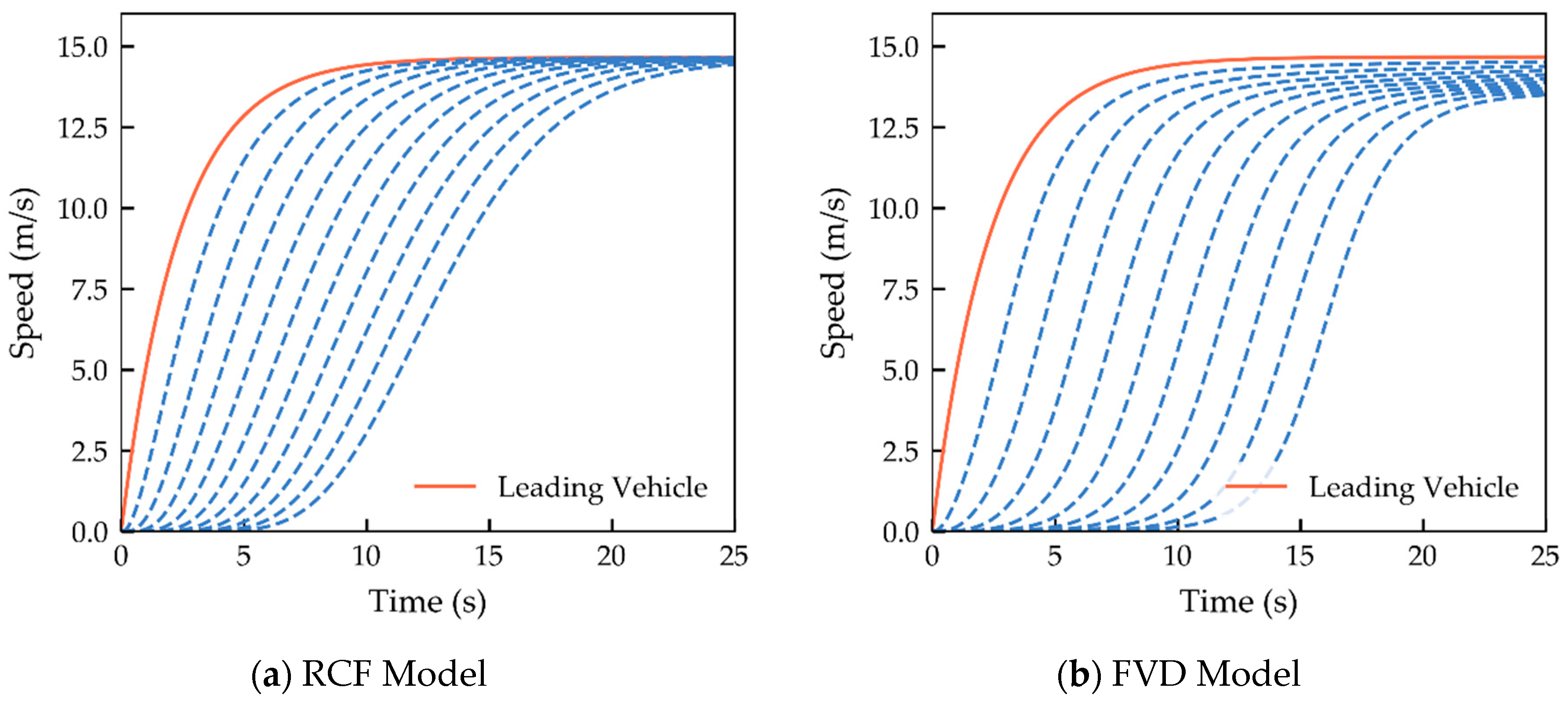
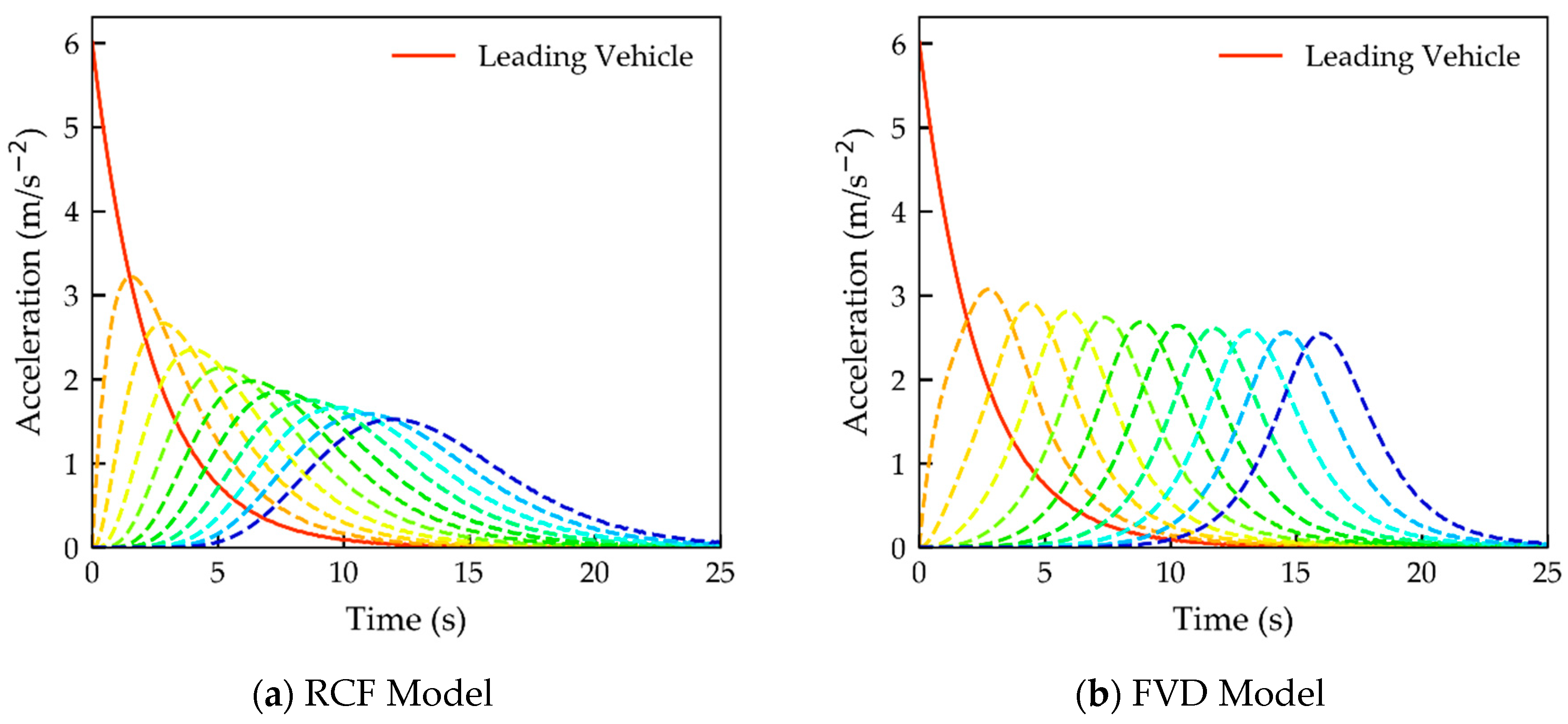
Assume that a car-following platoon of 11 vehicles waits with the same space headway of 7.4 m at a red traffic light, and the optimal velocity of each vehicle is zero. Then, at time $t=0$, the traffic signal becomes green and the leading vehicle will immediately start, and the other vehicles will gradually start. Figure 4 and Figure 5 show the evolution of the velocities and accelerations of the 11 vehicles during the starting process by different car-following models. Note that the solid lines in Figure 4, Figure 5, Figure 6, Figure 7, Figure 8 and Figure 9 represent the leading vehicle in the car-following platoon, and the dashed lines are the subsequent 10 vehicles.

By comparing the running information of the RCF model and the FVD model in the starting process, the following results were found:

(1) In the V2V communication environment, the RCF model only took approximately 20 s to render the velocities of the car-following platoon close to the preset maximum, which required less acceleration time than the FVD model.

(2) For the acceleration of the car-following platoon, the average acceleration of the car-following platoon simulated by the RCF model was smaller than that of the FVD model, and the acceleration from the leading vehicle to the last vehicle decreased more than that of the FVD model.

(3) The RCF model could start and accelerate the car-following platoon in 5 s, whereas the FVD model took approximately 10 s.

The reason for the above phenomenon was that the car-following platoon simulated by the RCF model could obtain the preceding vehicle’s running information in the V2V communication environment. For instance, when the first vehicle starts, its following vehicles will receive its running information at the same time, especially the speed information of the preceding vehicle. As a result, the driver can quickly start the vehicle, which reduces the delay time during the starting process. That is, since the driver knows the running information of the vehicles in the V2V covered region, they can have sufficient preparation time to start the vehicle. Therefore, the car-following platoon simulated by the RCF model can achieve gradual acceleration in a short time.

5.2. Braking Process

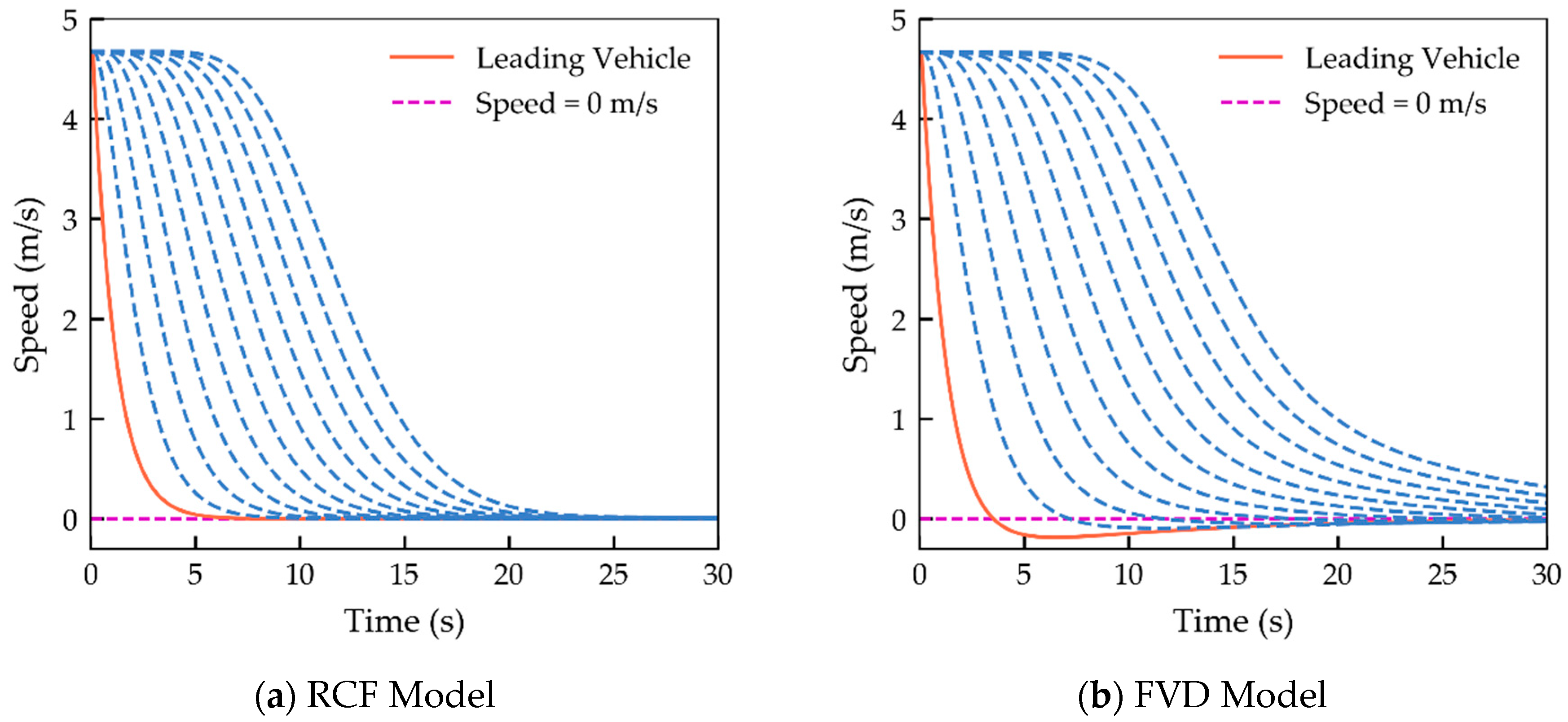
To explore the braking effect of the RCF model compared to the FVD model in consideration of drivers’ characteristics in the V2V communication environment, we supposed that 11 vehicles were running with the same space headway of 15 m and that each vehicle’s velocity was the optimal velocity ($V\left(15\right)=$4.67 m/s, as can be computed by Equation (1)). When $t=0$, the traffic signal becomes red and the leading vehicle will immediately brake, and the following vehicles begin to brake gradually. The braking process of vehicles is depicted in Figure 6, and the acceleration evolution of vehicles is depicted in Figure 7.

It can be seen from Figure 6 and Figure 7 that the running information simulated by the RCF model and the FVD model were more different during the braking process, as follows:

(1) Compared with the FVD model, the RCF model can completely stop in a shorter time. This effect is because the car-following platoon simulated by the RCF model can obtain the velocity information of the leading car earlier with the combination of V2V communication so that it can adjust its speed without delay to adapt to the current traffic situation. However, because the traditional OVF does not take into account the velocity of the preceding vehicle, the vehicles simulated by the FVD model do not stop immediately when the headway is small. Instead, these vehicles travel at a slower speed, as shown in Figure 6b, for 20 to 50 s.

(2) Although the deceleration of the leading vehicle simulated by the RCF model is higher than that of the FVD model, it still falls within a reasonable range [21].

(3) The space headway of the FVD model-simulated car-following platoon dropped to 7.3 m after 24 s, which was less than the set safe distance of 7.4 m. However, compared with the FVD model, the space headway of the simulated vehicles of the RCF model is much larger than the safety distance, which indicates that the RCF model can improve traffic safety. It is worth noting that existing studies have shown that many factors affect traffic safety, such as the characteristics of the driver, vehicle, crash, road, and environmental properties [54]. However, only the effects of drivers’ characteristics on the vehicle safety performance were explored during car-following in this study, and we assumed that other factors have a positive effect on traffic safety and will not reduce the safety performance of the vehicle.

5.3. Urgent Case

Urgent traffic cases are prevalent in real traffic scenarios, such as traffic accidents, emergency decelerations of preceding vehicles, and the sudden merging of vehicles in adjacent lanes. These incidents have a significant impact on regular running vehicles and may lead to abrupt changes in local traffic flow. In this subsection, we explore the effect of drivers’ characteristics with consideration of V2V communication on car-following behavior during an urgent case, and the following simulation scenario parameters are set. It is assumed that a platoon of 11 vehicles was distributed in the same lane with the same space headway (15 m), and that the initial optimal velocity of the platoon was uniformly 4.67 m/s. When $t=0$, the car 10 m in front of the leading vehicle suddenly stopped due to a traffic accident. At this time, the vehicles in the platoon started emergency braking beginning with the leading vehicle.

Figure 8, Figure 9 and Figure 10 depict the evolution of the velocity, acceleration, and space headway of vehicles in an urgent case. The following was found:

(1) The FVD model simulated a negative speed of the platoon; that is, the phenomenon of reversing was evident, which has been proven in the literature [23]. However, the RCF model did not appear to reverse. This finding was because, in urgent cases, the space headway of the preceding vehicle determined via the simulated FVD model decreases sharply, and its optimal velocity synchronization also decreases sharply. This decrease results in a significant change in the deceleration of the preceding vehicle, thereby making the preceding vehicle’s velocity rapidly decrease. Additionally, due to the limitation of the traditional OVF’s properties, when the space headway between the leading vehicle and the vehicle in which the accident occurred is small, a rapid deceleration cannot make the space headway larger than the safe distance. Therefore, the preceding vehicle simulated by the FVD model needed to be reversed to avoid a collision so that the distance between the preceding vehicle and the accident vehicle could be maintained at a safe distance. This phenomenon can be clearly seen from Figure 8 and Figure 10; the subsequent vehicles were successively impacted by the leading vehicle, and all vehicles demonstrated a reverse phenomenon.

(2) In unexpected events, the leading vehicles simulated by the RCF and FVD models both experienced high deceleration, but both fell within a reasonable range [21]. In addition, Figure 9 shows that the average deceleration of the simulated vehicles of the RCF model was greater than that of the FVD model. This result was because the RCF model can obtain the running information of the vehicles in the V2V covered region earlier so that emergency braking measures can be taken in time to avoid collisions.

(3) Vehicles simulated by the FVD model not only reversed in urgent cases, but the space headway of the platoon after the reversal was still smaller than the safe distance. However, each vehicle simulated by the RCF model could obtain traffic accident information earlier, so that it had sufficient time to deal with emergencies and could render an ideal space headway during emergency stops.

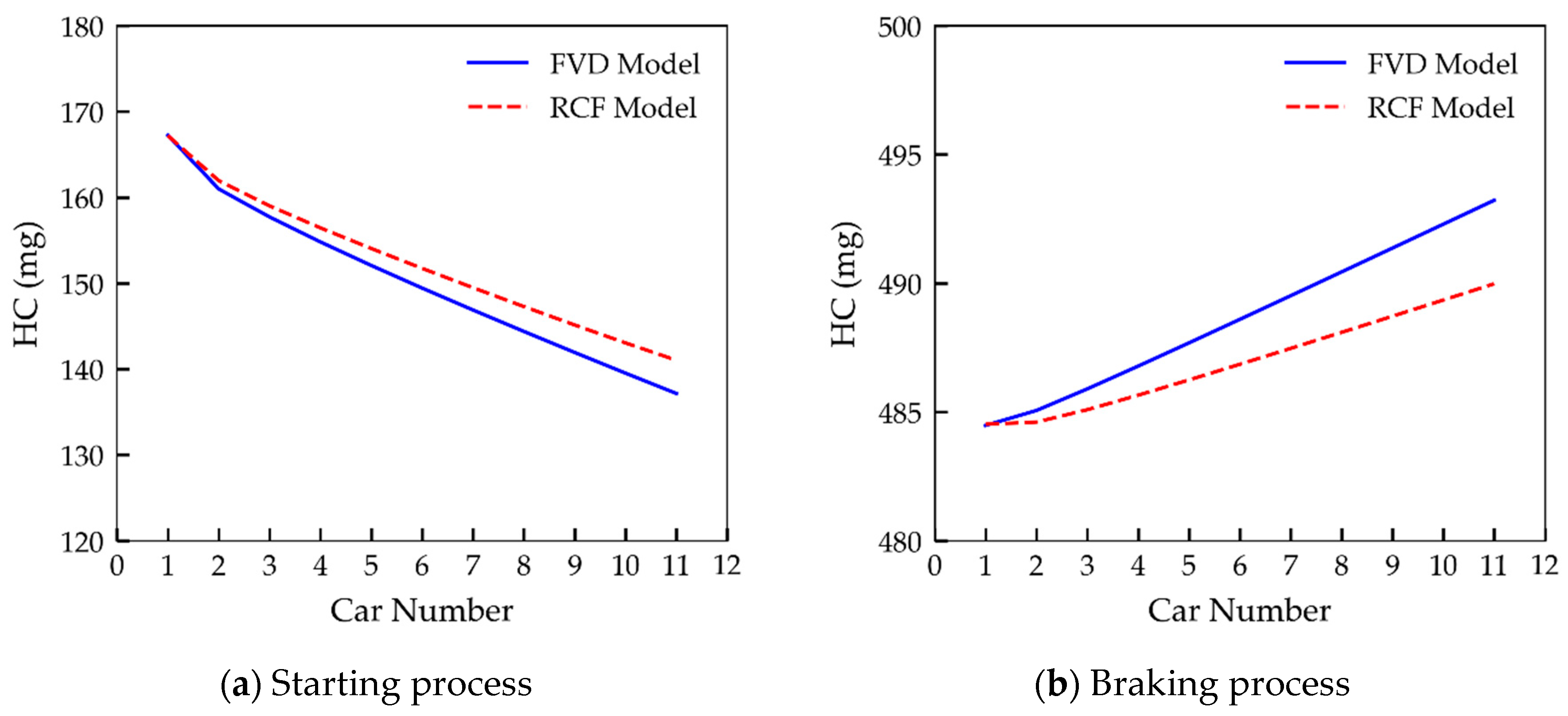
5.4. Fuel Consumption and Exhaust Emissions

Because the RCF model and FVD model cannot be directly used to evaluate the vehicle’s fuel and emission performance, in this section, we explore the fuel consumption and emissions of the aforementioned models in two typical traffic scenarios (starting process and braking process). The VT-Micro model proposed by Ahn et al. [55] can directly use the speed and acceleration to compute the vehicle’s instantaneous fuel consumption and exhaust emissions (i.e., carbon monoxide (CO), hydrocarbon (HC), oxides of nitrogen (NO_x)), and they pointed out that their model can perfectly fit the testing data. Therefore, the VT-Micro model was employed to estimate the fuel consumption and exhaust emissions of the aforementioned car-following model. The VT-Micro model can be formulated as follows:

$$\ln \left({\mathrm{MOE}}_e\right)=\{\begin{array}{cc}{\displaystyle {\displaystyle \sum }_{i=0}^3}{\displaystyle {\displaystyle \sum }_{j=0}^3}\left(L_{i,j}^e\times v^i\times a^j\right)& \mathrm{for} a\ge 0\\ {\displaystyle {\displaystyle \sum }_{i=0}^3}{\displaystyle {\displaystyle \sum }_{j=0}^3}\left(M_{i,j}^e\times v^i\times a^j\right)& \mathrm{for} a<0\end{array}$$

(13)

where ${\mathrm{MOE}}_e$ is the vehicle’s instantaneous fuel consumption (or exhaust emissions) rate, $L_{i,j}^e$ or $M_{i,j}^e$ is the corresponding regression coefficient [55], $v$ is instantaneous speed (m/s), and α is instantaneous acceleration (m/s²).

The model parameters for two typical traffic scenarios were consistent with those in Section 5.1 and Section 5.2. Therefore, the fuel consumption and exhaust emissions of vehicles simulated by the RCF model and FVD model can be computed by Equation (13), and the results are shown in Figure 11, Figure 12, Figure 13 and Figure 14. Thus, we can conclude the following results:

(1) From Figure 11a, Figure 12a, Figure 13a and Figure 14a, it can be found that the cumulative fuel consumption and exhaust emissions of the RCF model were greater than that of the FVD model during the starting process. The reason behind this is that during the starting process, the instantaneous speed and acceleration of each vehicle increased sharply for the purpose of fast starting, which inevitably increased the vehicle’s fuel consumption and undermined the emissions performance [56,57]. However, it can be seen from

Table 2. The total fuel consumption and emissions of the car-following platoon during the starting processes.

	Fuel Consumption (mL)	CO (mg)	HC (mg)	NOx (mg)
FVD Model	1956.52	13,725.62	1652.17	1811.94
RCF Model	2002.18	14,443.73	1676.40	1860.60
$∆\left(RCFM-FVDM\right)$	45.66	718.11	24.23	48.66

that although the total fuel consumption and exhaust emissions of the RCF model were greater than that of the FVD model, the differences between them were very small. In addition, it is important notice the fact that the RCF model took less time to reach the maximum speed during the starting process than the FVD model, which was confirmed in Section 5.1. Therefore, the overall performance of the RCF model may be better during the starting process.

(2) From Figure 11b, Figure 12b, Figure 13b and Figure 14b, it can be clearly found that the fuel consumption or exhaust emission performance of the RCF model was better than that of the FVD model during the braking process. It shows that the RCF model can save more energy and reduce exhaust emissions. In addition, compared to the FVD model, the RCF model could also make the vehicle stop more quickly without reversing. It can be concluded that the RCF model can not only optimize vehicle’s mobility and safety in different traffic scenarios, but also reduce vehicles’ fuel consumption and promote emission performance. More importantly, these results may have potential theoretical values for improving the operational efficiency and promoting the sustainable development of the transportation system.

6. Conclusions

With the deployment of intelligent transportation systems and the improvement in the performance of in-vehicle communication equipment, drivers can obtain traffic information from multiple preceding vehicles. Therefore, on the basis of the vehicle trajectory data from the NGSIM project, this study proposed a car-following model with V2V communication technology that took into account drivers’ characteristics. First, by exploring the properties of the traditional OVF [20] and real car-following data, it was found that the driver’s optimal velocity depended not only on the space headway but also on the velocity of the preceding vehicle. To quantify the above relationship, we used the grey relational analysis method to determine the factors that significantly impact the driver’s optimal velocity and established a new OVF. The new OVF had more boundary conditions than the traditional OVF, which was in line with the characteristics of drivers in traffic situations. Furthermore, the properties of the new OVF were theoretically proven in this paper. Considering the superior properties of the new OVF, on the basis of the FVD model, an extended car-following model that considers drivers’ characteristics in a V2V communication environment was proposed, and the properties of the proposed model were analyzed qualitatively.

To evaluate and validate the performance of the proposed model, the FVD model was selected as a control model, and three different simulation scenarios were designed to analyze the aforementioned models. Before starting the numerical simulation experiments, we provided the basic assumptions and model simplification methods under the V2V communication environment. The simulation results showed that the RCF model proposed in this paper required less time during the starting process and braking process than the FVD model. Moreover, the RCF model could accelerate the entire platoon to a set maximum speed faster during the starting process and could also quickly stop during the braking process. In addition, in the event of an accident, the RCF model not only avoided reversing but also maintained the space headway of the platoon at an ideal level to avoid collisions.

Numerical simulations revealed that the proposed model could improve vehicles’ mobility, safety, fuel consumption, and emission performance compared to the FVD model, and the RCF model could readily describe some critical car-following conditions that are consistent with real-world situations. For example, because drivers can obtain more traffic information earlier, they can make accurate decisions in time to avoid collisions or traffic jams. As a result, the safety and comfort of vehicles running on the road could be improved to varying degrees. It is worth noting that because the proposed model can improve the traffic stability, safety, and fuel economy, these advantages have a positive effect on improving vehicle fuel consumption and emissions performance [58]. In other words, this study provides potential contributions to the improvement of the operational efficiency and promotion of the sustainable development of transportation systems. In addition, this study assumed that vehicles transfer traffic information in real time through V2V communication technology. However, due to the limitations of the current level of traffic information technology, there may be transmission delays and data packet losses of running information in vehicle-to-vehicle and vehicle-to-infrastructure communication, which may cause the following vehicle to not receive the running information of the preceding vehicle in time. Therefore, our next study will consider the characteristics of traffic flow under delay factors, such as packet losses or transmission delays.