The Spatial Spillover Effect in Hi-Tech Industries: Empirical Evidence from China

Abstract

With ever-increasing economic globalization and rapid advancement of science and technology, developing high-tech industries have become an important way for many countries to achieve sustainable and environmentally friendly economic development. In this article, we aim to empirically test the critical factors, which can influence the spatial spillover of a country’s high-tech industries. Using data from the high-tech industries in China during the years of 2007–2016, we establish a space lag model and a space error model to examine the space fixed effect, the time fixed effect, and the space-time double mixed effect in spatial spillover in high-tech industries. We compare the results of these two spatial panel models with those from a general panel model and find that the spatial spillover effect within high-tech industries is rather significant. Moreover, we find that the spatial-time double mixed of the spatial lag model is the best fitting effect. Our empirical results also show that the research and development (R&D) investment and international trade can positively promote spatial spillover of high-tech industries among different regions. In terms of policy insights, our results imply that the government can establish a technology transfer platform to promote the spillover in high-tech industries. This can help achieve a sustainable and balanced development of high-tech industries.

1. Introduction

The development of high-tech industries has been of great strategic significance for countries to cope with the ever-changing international market competition. As a result, many countries such as China have implemented strategic plans for the development of high-tech industries. Therefore, it is of great importance to study the contributing factors, which can help further improve the performance of high-tech industries and promote the transformation into a more knowledge-based economy.

There has been steady research on the performance of high-tech industries and its critical factors. For example, Reference [1] studies the research and development (R&D) activities of Spanish enterprises and found that R&D activities can greatly impact the performance of product innovation [1]. However, the impacts of external resources on the performance of high-tech industries and manufacturing industries are very different. Reference [2] adopts the Malmquist productivity index to measure the total factor productivity of the high-tech industry. Reference [3] shows that there exist salient spatial agglomeration effects in the high-tech enterprises. In this paper, we focus on the following important questions: what are the critical factors which can influence the spatial spillover of high-tech industries? How do these factors influence the spatial spillover? What are the potential reasons for the unbalanced regional development of high-tech industries? The answers to these questions are of great theoretical and practical significance because they can help improve the output of the high-tech industries and promote the sustainable and balanced development of regional economies for many countries. For example, China is a vast country with regions with unbalanced economic development. The high-tech industries are highly concentrated in only several developed regions like Guangdong Province. How do you achieve the spillover of high-tech industries to other underdeveloped regions? This question is important not only for China’s economic development, but also for many countries in the world with unbalanced regional economic development.

In this paper, we employ spatial panel models to study spatial spillover in high-tech industries. We adopt the spatial panel models because they can deal with the spatial dependence among regions. In contrast, traditional models such as Ordinary Least Squares (OLS) models ignore the spatial effect and lead to estimation errors. To be more specific, in this research, we employ the spatial lag model (SLM) and the spatial error model (SEM), which are two of the most widely used spatial panel models. The SEM focuses on the influence of the error of random interferences, while the SLM focuses on the existence of spatial spillover among regions.

This paper makes the following contribution to the literature. First, by explicitly incorporating spatial factors, the study extends existing research and contributes to our understanding on the spatial spillover in high-tech industries. Second, our research helps understand the possible causes for unbalanced spatial distribution of high-tech industries. Third, this research provides policy insights on how to develop more sustainable and balanced high-tech industries.

The rest of the paper is arranged as follows. Section 2 reviews the existing studies. Section 3 describes the data source and variables. Section 4 establishes the theoretical models. Section 5 presents the empirical analysis and results. Section 6 concludes the paper and proposes policy implications and potential future research.

2. Literature Review

This study is mainly associated with three research streams. First, the study is related to how new technologies can lead to spatial agglomeration in industries. Reference [4] analyses the extent to which the spatial distribution of the economy promotes innovation using patent data from India from 1997 to 2007. Through quantitative research, it concludes that human resources, industrial diversity, and R&D expenditure critically impact the spatial distribution of technological innovation. Reference [5] examines the geographical distribution of entrepreneur networks. It demonstrates that the impact of geographic network diversity on the enterprises’ exploratory innovation level is inverted and U-shaped. Reference [6] proves that the spatial characteristics of collaboration in knowledge creation can change dramatically in a relatively short period of time through the analysis of the social network of Master Boot Record (MBR) technical data. Reference [7] argues that reorganization is a process of combining different fields of knowledge creatively in an invention. Different dimensions of partner proximity affect the probability of cooperative innovation. Moreover, geographical proximity has an inverted U-shaped effect on restructuring innovation.

Second, this study is also related to the literature on the impact of knowledge production and transfer. High-tech industries are mostly located in regions where knowledge production is active and innovation activities are heavily invested. Reference [8] shows that the common characteristics of regions with high-tech industry agglomeration have high R&D investment, efficient venture capital channel, frequent activities of corporate alliance, and entry of a large number of professionals in these regions. Through the research of 45 biomedical companies gathered in the same region, Reference [9] demonstrates that knowledge production is the source of innovation. Based on European Union patent data, Reference [10] points out the spatial flow of innovators causes the flow of knowledge, which, in turn, promotes the agglomeration of high-tech activities. Reference [11] explores the determinants of cooperation between enterprises and universities, and whether they differ according to the technological level of the enterprise. Reference [12] argues that high-tech activities will change with time in the dynamic and uncertain technological environment. Its analysis of patent data shows a collaboration mechanism affects firm performance. Moreover, the role of the collaboration mechanism is also affected by the technological specialization of enterprises. Reference [13] proposes a new model to evaluate the opportunities of an industrial economic structure and uses the concept of “product space” to evaluate the technological penetration and complexity of different production sectors. Reference [14] studies how technological progress and migration costs interact to shape the spatial economy. Reference [15] proposes that total factor productivity (TFP) is not only a measure of long-term economic growth, but also a comprehensive index of industry-level productivity. Reference [16] argues that government policies and regulations related to high-tech industries should protect promising new technologies and support the cumulative process of market formation and growth.

Third, this study is related to the research stream on how organizational structures impact the flow of ideas, resources, technology, personnel, and the spatial spillover of industries. Reference [17] analyzes why ecotype organization space is important for technology catching-up by comparing China’s leading automobile groups. Reference [18] combines the genetic model with the knowledge model and its experimental results reveal that technological innovation of complex products is one of the most effective ways to build future core competitiveness. Reference [19] clarifies the organizational process of generic technology design and describes it through uncertain experimental evolutionary strategies. Based on the viewpoint of the evolution theory and Schumpeterian economics, Reference [20] holds that “innovation space” should focus on the search process, which can affect the opportunities in specific geographical environments. Reference [21] believes that the evolution of product space has a strong path dependence, but the heterogeneity in scale, efficiency, and international exposure impacts this dependence. Reference [22] demonstrates that knowledge spillover is related to geographical proximity. Its results show that knowledge spillovers in Europe occur through geographic, relational, social, cognitive, and technological channels.

In summary, although much research has been done on the impact of agglomeration and distribution of high-tech industries, there are still gaps in the existing research. First, because of the regional unbalance in the high-tech industries in many countries such as China, spatial factors may be key. Therefore, this study adds the spatial factors and explores the spatial spillover effect based on spatial panel models. Second, although there are several studies on the spatial agglomeration of high-tech industries from the perspectives of R&D, knowledge flow, organizational change, and new technologies, few studies focused on the spatial spillover effect of high-tech industries from the perspectives of international trade and technological capacity development. This study incorporates these two perspectives.

3. Data and Spatial Correlation Analysis

3.1. Data Source

In this paper, we collect panel data from the high-tech industries of China from the years between 2007 and 2016, including the four municipalities directly under the Chinese Central Government and 24 provinces. The four municipalities are Beijing, Shanghai, Tianjin, and Chongqing. The 24 provinces include Hebei, Shanxi, Inner Mongolia, Liaoning, Jilin, Heilongjiang, Jiangsu, Zhejiang, Anhui, Fujian, Jiangxi, Shandong, Henan, Hubei, Hunan, Guangdong, Guangxi, Hainan, Sichuan, Guizhou, Yunnan, Shaanxi, Gansu, and Ningxia. The four provinces of Xinjiang, Tibet, and Qinghai are excluded because of the absence of their data in the statistical yearbook. These data involve the main business income, the number of full-time R&D personnel, R&D expenditure, export delivery value, new product development expenditure, and technology upgrading expenditure. The data sources include Statistical Yearbook of China and Statistical Yearbook of High-Technology Industry compiled by the National Bureau of Statistics of China. The new product development expenditure refers to the expenditure for the research and development of new products in the scientific and technological activities. The technology upgrading expenditure involves the application of scientific and technological advancements in production, the upgrading of more advanced technology and equipment, and the implementation of product upgrading and energy conservation.

3.2. Variables

When selecting indicators, we follow References [23,24,25] and choose the main business income to measure the output of high-tech industries in each region. The data on the main business income are from 2007 to 2016, which is convenient for spatial econometric regression. In terms of independent variables, we choose the number of full-time R&D personnel and R&D expenditure as the R&D investment factor, which is used to measure the actual investment in R&D [26]. We use export delivery value to measure the impact of international trade, which is an important index to measure the products entering the international market. It is also the main parameter to measure the extent to which high-tech enterprises are integrated into the world economy [27,28]. New product development expenditure and expenditure technology upgrading expenditure are two important indicators to measure technology development capability [29].

Table 1. Variables and their definitions.

Variable	Definition	Unit
MBI	The main business income of the high-tech industries	10,000 Yuan
RDP	The number of full-time R&D personnel	Person/Year
RDF	R&D expenditure	10,000 Yuan
EDV	Export delivery value	10,000 Yuan
NPD	New product development expenditure	10,000 Yuan
TRF	Technology upgrading expenditure	10,000 Yuan

summarizes the definitions of these variables.

3.3. Global Spatial Correlation

The global spatial correlation is used to measure the correlation and significance of the interval population, which is expressed by Moran’s I index [30]. Moran’s I also reflects the degree of global correlation. Generally speaking, the larger Moran’s I is, the stronger the global correlation is. The mathematical formulation of Moran’s I is as follows:

$$I=\frac{{{\displaystyle \sum }}_{\mathrm{i}=1}^n{{\displaystyle \sum }}_{\mathrm{j}=1}^n{W}_{\mathrm{ij}}\left(Y_i-\overline{Y}\right)\left(Y_j-\overline{Y}\right)}{S^2{{\displaystyle \sum }}_{\mathrm{i}=1}^n{{\displaystyle \sum }}_{\mathrm{j}=1}^n{W}_{\mathrm{ij}}}$$

(1)

where ${\mathrm{S}}^2=\frac{1}{\mathrm{n}}{{\displaystyle \sum }}^{\text{}}\left({\mathrm{Y}}_{\mathrm{i}}-\overline{\mathrm{Y}}\right)$. The total number of space units involved in the calculation is $n$. The space weight matrix is expressed by $W$. Moran’s I has a range of values from −1 to 1, and can be inferred from the test value Z.

$$Z=\frac{I-E\left(I\right)}{\mathrm{SD}\left(I\right)}$$

(2)

In Equation (2), the expected return is expressed as E(I). The standard deviation is expressed as SD(I). In our research, the meaning of Z is that, when Moran’s I is positive and the significance is good, it shows that the regions with high innovation output are adjacent to each other. When Moran’s I is negative and the significance is very high, it indicates that there is a large difference among adjacent regions. That is, a region with high innovation output is adjacent to a region with low innovation output.

When calculating Moran’s I index, the spatial weight matrix $W$ is needed, and the vehicle-type spatial weight matrix is generally selected. Based on the calculation rule of the vehicle-type spatial weight matrix, if two spatial elements have a common boundary, it means that they are “adjacent.” If there is no common boundary, it means that they are “non-adjacent.” Figure 1 shows an example of the vehicle-type spatial weight matrix [31].

In the matrix shown in Figure 1, 1 and 0 mean that space unit i and space unit j are adjacent and non-adjacent, respectively. For our data, the results of Moran’s I values are shown in

Table 2. Moran’s I values.

Year	Moran’s I	p-Value
2006	0.11 *	0.10
2007	0.28 *	0.08
2008	0.21 *	0.09
2009	0.25 *	0.06
2010	0.31 *	0.09
2011	0.32 **	0.03
2012	0.36 ***	0.00
2013	0.39 **	0.03
2014	0.41 ***	0.00
2015	0.41 ***	0.01
2016	0.41 ***	0.00

* denotes significance at the 10% level. ** denotes significance at the 5% level. *** denotes significance 1% level.

.

It can be seen from Table 2 that the global spatial correlation has been significantly increased in the past 10 years. The results of Moran’s I values indicate a steady upward trend, which means that the increase of spatial correlation also intensifies the agglomeration of high-tech industries. Moreover, the development of the high-tech industries in each province has mutual influence in space. The closer the innovation level is, the more high-tech industries tend to gather together.

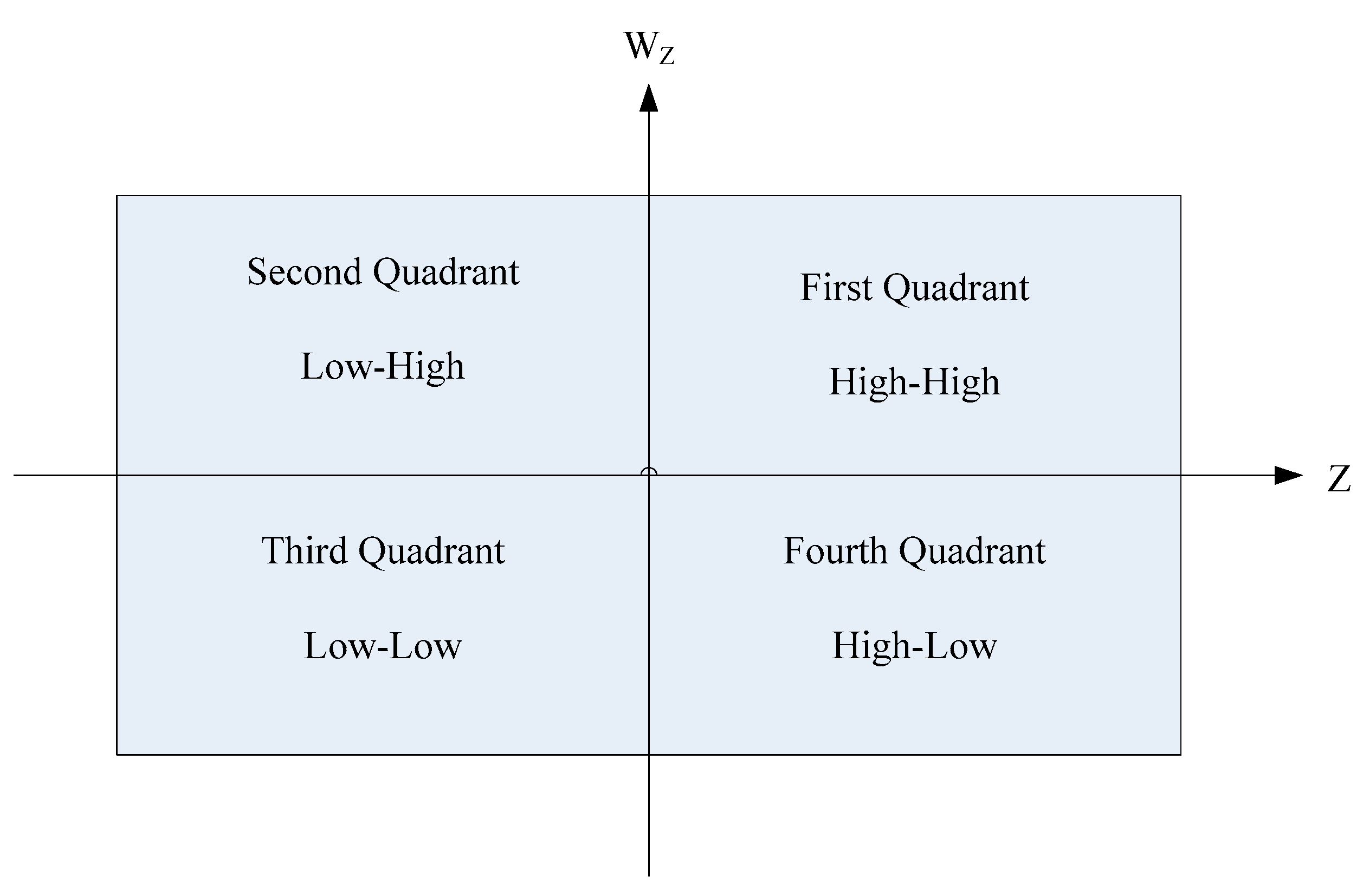
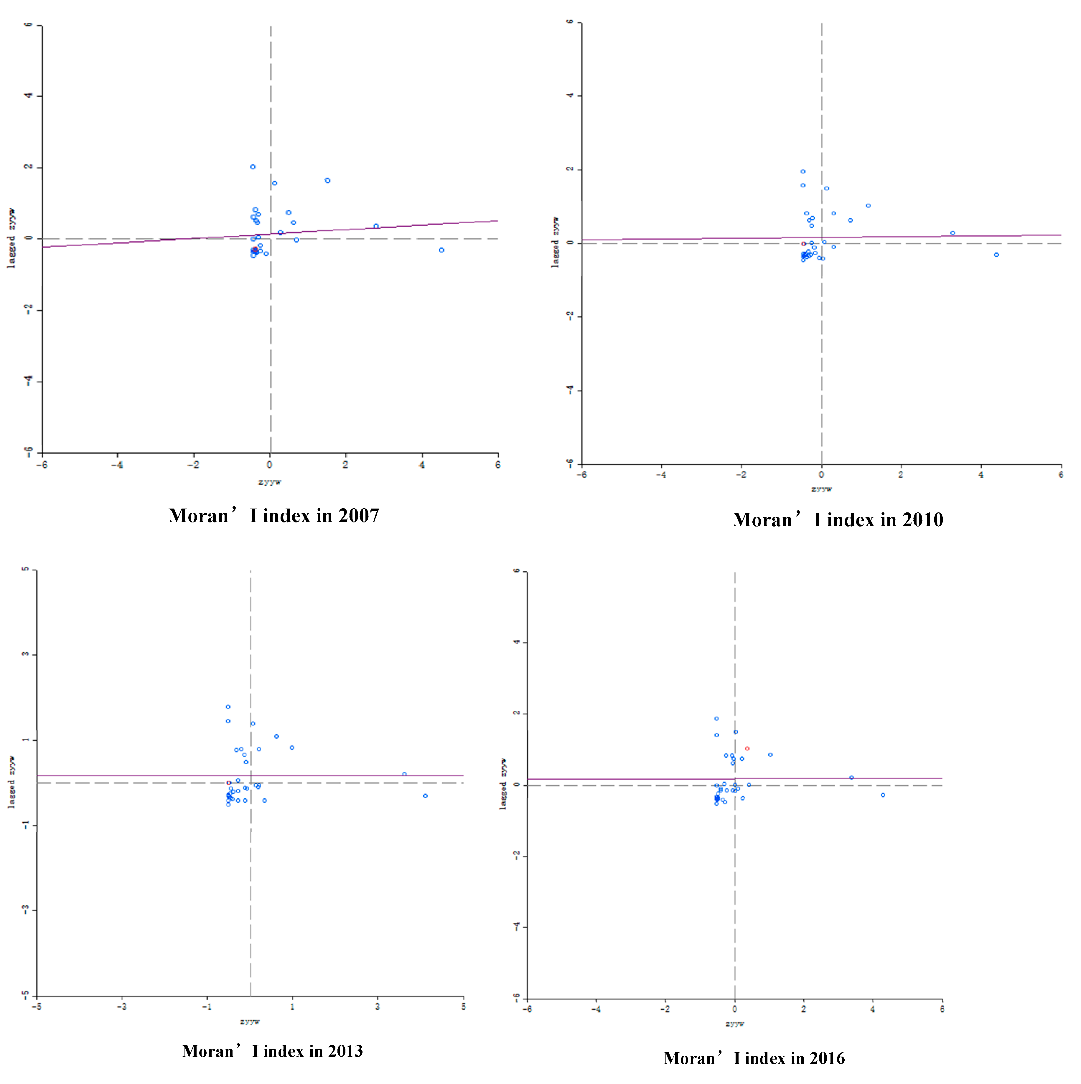
3.4. Local Spatial Correlation Analysis

Local spatial correlation analysis focuses on the relationship between a spatial unit and its surrounding units. In addition, the most widely used tool is the Moran scatter diagram. It uses a two-dimensional graph to express the relationship between a space unit and its surrounding space units [32]. If Z is used to represent a space unit and its surrounding space unit is $W_Z$, then Z and $W_Z$ constitute four quadrants, which are illustrated in Figure 2.

The first quadrant is a quadrant with a fully positive correlation, which indicates the agglomeration of regions with high innovation output. The third quadrant is the quadrant with a fully negative correlation, which indicates the agglomeration of regions with low innovation output. The second quadrant represents the scenario where a region has low innovation output, but its neighbors have high innovation output. Lastly, the fourth quadrant represents the scenarios where a region has high innovation output, but its neighbors have low innovation output [33].

With an interval of three years, we use the ArcGIS software to plot the trend of the Moran’s I values for China’s high-tech industries from 2006 to 2016, as shown in Figure 3.

Figure 3 conveys two important messages. First, the innovation of local regions shows the characteristics of strong spatial agglomeration. That is, the regions with high innovation are more closely gathered. Furthermore, the degree of a spatial difference between regions is expanding. Second, the spatial connection between regions is strengthening every year.

4. Research Models

4.1. Introduction of the Spatial Econometric Model

The Spatial Error Model (SEM) and Spatial Lag Model (SLM) are two different types of spatial econometric models. The idea of the SLM model is to discuss whether there is spatial spillover or spillover among regions. It uses a parameter to measure the impact of adjacent regions. The main idea of the SEM model is to calculate the influence of a random interference term on the regional observation value. Specifically, the SEM model is expressed as the following:

$$y=x\beta +\epsilon ; \epsilon =\lambda W{\epsilon }_i+\mu$$

(3)

where $x$ is an explanatory variable and a $n\ast k$ matrix. $y$ is a dependent variable. $\beta$ is the coefficient of explanatory variables. $\epsilon$ is a random error vector and $\lambda$ is a spatial error coefficient. The main function is to measure the degree of interdependence of different spatial samples, that is, the influence of observation values of adjacent regions on the spatial unit. The SLM model can be expressed as follows.

$$y=\rho Wy+x\beta +\epsilon$$

(4)

where $\rho$ is a spatial regression coefficient, which explains the influence of an adjacent observation value. $W$ is a spatial weight matrix. $\beta$ is a dependent variable coefficient. $\epsilon$ is the random error term of the model.

When considering both temporal and spatial effects, we need to combine the general panel data model with the spatial econometric model. As a result, we can obtain the following spatial lag regression model based on panel data (time effect).

$$y_{it}={\alpha }_{it}+\rho W{y}_{it}+x_{it}\beta +{\epsilon }_{it}$$

(5)

where $t=1,2,\dots t_i$ and $i=1,2,\dots n$. In Equation (3), $y_{it}$ represents the dependent variable at time t. ${\alpha }_{it}$ is a non-observational effect, which does not change with time. $\rho$ is a spatial regression coefficient. $w{y}_{it}$ is the dependent variable of space lag at time t. $\beta$ is the coefficient of the independent variable $x_{it}$. For every unit of $y_{it}$, $x_{it}$ will change $\beta$ units. Similarly, the spatial error regression model based on panel data (time effect) is shown below.

$$y_{it}=x_{it}\beta +{\epsilon }_{it}$$

(6)

$$\epsilon =\lambda W{y}_{it}+{\epsilon }_{it}+\mu$$

(7)

In choosing spatial econometric models, researchers mainly use the discriminant method proposed in Reference [34]. Several important indicators to measure the validity of the model are Moran’s value, Lagrange Multipher’s space lag (LM Lag), and space error (LM error), and the robustness of space lag and a space error model. The corresponding parameters are Robust-LM lag and Robust-LM error. The principle of discrimination is to decide which model is more suitable according to the significance between the contrast indicators. For example, if the spatial error model is more significant than the spatial lag model, and the robustness of the spatial error model is also very significant, then the spatial error model is more suitable than the spatial lag model. Similarly, if LM (lag) is more significant than LM (error), and Robust LM (lag) is significant while Robust LM (error) is not, then the spatial lag model is appropriate.

4.2. Spatial Model

The existing literature has commonly adopted the following Knowledge Production Function model to explore the driving force of knowledge production and spillover among regions [35]:

$$Q_{it}=A{K}_{it}^{\alpha }{L}_{it}^{\beta }{\epsilon }_{it}$$

(8)

The model (8) employs the form of a Cobb-Douglas production function, which was first proposed in Reference [36] and later extended and improved in Reference [37]. In model (8), innovation output is denoted by $Q_{it}$. $A$ denotes the technical level of the society. R&D expenditure is denoted by $K_{it}$. Labor input is denoted by $L_{it}$. Random error is denoted by ${\epsilon }_{it}$. Moreover, by adopting model (8), we implicitly assume that the firms are efficient and endogenous. Future research can consider the scenarios where these assumptions are not satisfied. To eliminate heteroscedasticity, all variables are processed by a logarithm and we have the following:

$$ln{Q}_{it}=lnA+\alpha ln{K}_{it}+\beta ln{L}_{it}+{\epsilon }_{it}$$

(9)

In the literature review of this article earlier, we discuss the factors that may influence the output of high-tech industries. In addition, References [38] show that technology and social factors may influence the main business income. These factors include export delivery value, new product development expenditure, and technology upgrading expenditure. Hence, we first add all these variables to construct the STRIPAT (Stochastic Impacts by Regression on Population, Affluence, and Technology) model without considering spatial factors. The basic panel model without considering spatial factors is shown below.

$$lnMB{I}_{it}={\alpha }_1+{\beta }_{1}lnRD{P}_{it}+{\beta }_{2}lnRD{F}_{it}+{\beta }_{3}lnED{V}_{it}+{\beta }_{4}lnNP{D}_{it}+{\beta }_{5}lnTR{F}_{it}+{\epsilon }_{it}$$

(10)

The business income of high-tech industries in a region is affected not only by R&D personnel, R&D expenditure, export value, new product development, and technological upgrading, but also by the economic growth in the surrounding regions. Hence, the spatial effects of the industrial structure are investigated using spatial panel data models. Similar to Reference [39], the spatial error models can be constructed by using the equations below.

$$lnMBI={\alpha }_1+wlnMB{I}_{it}+{\beta }_{1}lnRD{P}_{it}+{\beta }_{2}lnRD{F}_{it}+{\beta }_{3}lnED{V}_{it}+{\beta }_{4}lnNP{D}_{it}+{\beta }_{5}lnTR{F}_{it}+{\epsilon }_{it}$$

(11)

$$\epsilon =\lambda wlnMBI+\mu$$

(12)

$$\mu ~N\left(0,{\sigma }^2\right)$$

(13)

Following Reference [40], the spatial lag model can be constructed using the equation below.

$$\begin{gathered} lnMBI={\alpha }_1+\rho {\displaystyle \sum }_{j=1}^n{w}_{ij}lnMB{I}_{it}+{\beta }_{1}lnRD{P}_{it}+{\beta }_{2}lnRD{F}_{it}+{\beta }_{3}lnED{V}_{it} \\ +{\beta }_{4}lnNP{D}_{it}+{\beta }_{5}lnTR{F}_{it}+{\epsilon }_{it} \end{gathered}$$

(14)

5. Empirical Results

5.1. Estimation of Non-Spatial Panel Models

The traditional panel models generally do not consider spatial factors. In addition, there is no spatial lag in the dependent variable and there is no spatial error autocorrelation [41].

In

Table 3. Estimation results of the general panel model.

Variable	Coefficient	Std. Error	t-Statistic	Prob
$\mathit{\alpha }$	−1.26 *	0.68	−1.86	0.06
$\mathit{L}\mathit{n}\mathit{R}\mathit{D}\mathit{P}$	−0.20	0.13	−1.48	0.14
$\mathit{L}\mathit{n}\mathit{R}\mathit{D}\mathit{F}$	0.22	0.17	1.27	0.20
$\mathit{L}\mathit{n}\mathit{E}\mathit{D}\mathit{V}$	0.24 ***	0.06	3.84	0.00
$\mathit{L}\mathit{n}\mathit{N}\mathit{P}\mathit{D}$	0.59 ***	0.14	4.11	0.00
$\mathit{L}\mathit{n}\mathit{T}\mathit{R}\mathit{F}$	−0.11 **	0.06	−1.90	0.06
Adj-${\mathit{R}}^{\mathbf{2}}$	0.50
S.E. Regression	0.96
Durbin-Waston	0.33

* denotes significance at the 10% level. ** denotes significance at the 5% level. *** denotes significance 1% level.

, the fitting coefficient of the model is only 0.4987, which is relatively low. According to the empirical test results, only export delivery value and new product expenditure are the significant independent variables. The other three variables, namely, the number of full-time R&D personnel, R&D expenditure, and technology upgrading expenditure, are insignificant. Therefore, the effect estimated by the general panel model is not ideal. According to Reference [42], this indicates that there may be a spatial interaction between variables, which we need to verify further.

5.2. Estimation of the Spatial Lag Model

The Spatial Lag Model (SLM) was calculated by using MATLAB 7.0. The estimation results are summarized in

Table 4. Estimation results of the SLM.

Variable	Spatial Fixed Effect	Time Fixed Effect	Spatial-Time-Double-Mixed Effect
$\mathit{L}\mathit{n}\mathit{R}\mathit{D}\mathit{P}$ Ln(RDP)	−0.13 (−0.99) [0.32]	−0.13 (−0.71) [0.48]	0.13 ** (1.12) [0.06]
$\mathit{L}\mathit{n}\mathit{R}\mathit{D}\mathit{F}$ Ln(RDF)	0.12 (0.79) [0.43]	−0.30 (−1.26) [0.21]	0.20 ** (−1.29) [0.07]
$\mathit{L}\mathit{n}\mathit{E}\mathit{D}\mathit{V}$ Ln(EDV)	0.21 *** (3.49) [0.00]	0.26 *** (4.44) [0.00]	0.11 ** (2.04) [0.04]
$\mathit{L}\mathit{n}\mathit{N}\mathit{P}\mathit{D}$ Ln(NPD)	0.44 *** (3.28) [0.00]	0.50 ** (2.36) [0.02]	−0.00 (−1.24) [0.22]
$\mathit{L}\mathit{n}\mathit{T}\mathit{R}\mathit{F}$ Ln(TRF)	−0.10 * (−1.96) [0.05]	0.04 (0.51) [0.61]	−0.00 (−0.02) [0.98]
${\mathit{R}}^{\mathbf{2}}$R2	0.91	0.79	0.95
${\mathit{\sigma }}^{\mathbf{2}}$	0.79	2.11	0.64
Log-likelihood	−584.53	−808.06	−536.35

* denotes significance at the 10% level. ** denotes significance at the 5% level. *** denotes significance 1% level. () represents the t-test value. [] represents the probability value corresponding to the t-test value.

.

The estimation results can be divided into three categories: the spatial fixed effect, the time fixed effect, and the space-time mixed effect. According to Elhorst [38], when choosing the model, we need to determine the type of model including the space fixed effect model, the time fixed effect model, or the time space double fixed effect model. The spatial fixed effect model adopts different intercept terms for different time series (individuals). The time fixed effect model adopts different intercept terms for different sections (time points). Furthermore, the time space double fixed effect adopts different intercept terms for different sections (time points) and different time series (individuals). However, this research uses the software of MATLAB, which automatically test all three models. As a result, we can simply identify the best-fitting model based on the significance and log likelihood value.

From the regression results, the fitting value of the mixing effect is the best at 0.9467. In the estimation of a maximum likelihood ratio coefficient, it is also the best value of the mixing effect, which reaches −536.3519. Judging from the significance of variables, the number of R&D personnel, R&D expenditure, and export delivery value are significant. Furthermore, these three variables are positively correlated with the y value such as the main business income. Two variables, which include the new product development expenditure and the technology upgrading expenditure, are insignificant. Moreover, their coefficients are negative, which indicates that these two factors may have negative relationships with the spillover effect of high-tech industries.

5.3. Estimation of the Spatial Error Model

Similarly, a panel data-based Spatial Error Model (SEM) is established. The estimation results are summarized in

Table 5. Estimation results of the SEM.

Variable	Spatial Fixed Effect	Time Fixed Effect	Spatial-Time-Double Fixed Effect
Ln(RDP)	−0.11 (−0.84) [0.40]	−0.16 (−0.88) [0.38]	0.13 (1.10) [0.27]
Ln(RDF)	0.17 (1.01) [0.31]	−0.17 (−0.70) [0.48]	−0.19 (−1.23) [0.22]
Ln(EDV)	0.23 *** (3.95) [0.00]	0.22 *** (3.54) [0.00]	0.12 *** (2.13) [0.03]
Ln(NPD)	0.56 *** (4.16) [0.00]	0.56 *** (2.59) [0.01]	−0.22 (−1.41) [0.16]
Ln(TRF)	−0.08 (−1.34) [0.18]	−0.06 (−0.77) [0.44]	−0.03 (−0.61) [0.54]
$\mathit{\lambda }$	0.05 (0.59) [0.56]	−0.28 *** (−2.94) [0.00]	−0.13 * (−1.65) [0.10]
R2	0.40	0.41	0.79
Log-likelihood	−590.94	−814.27	−535.56
${\mathit{r}}^{\mathbf{2}}$r2	0.40	0.411	0.29
${\mathit{L}}_{\mathit{i}}$Li	−590.94	−814.27	−535.56
AkaikeInformationCriterion(AIC)	1195.88	1642.54	1085.13
Bayes Information Criteria(BIC)	1224.62	1671.28	1113.86

* denotes significance at the 10% level. *** denotes significance 1% level. () represents the t-test value. [] represents the probability value corresponding to the t-test value.

.

From the results listed in Table 5, we can see that the fitting value R² of the estimation effect of regression is not very high, and the best of the spatial-time mixed effect is only 0.7898. The maximum likelihood mixing effect is −535,5630. In terms of the significance, only the export delivery value passed the 1% significance test and all other variables were insignificant. Comparing the estimation results of the SEM and the SLM, we can see that the SLM is better than the SEM. This indicates that there is very strong spatial spillover or a spatial spillover effect in the high-tech industries. In other words, a region’s high-tech output will be greatly impacted by its adjacent regions.

5.4. Discussions

In the literature, Reference [43] examines how foreign direct investment (FDI) spurs entrepreneurial activity in host countries. It also investigates why this relationship varies across countries because of domestic socio-political conditions. Reference [44] shows the role of technology spillovers in productivity growth of Organization for Economic Co-operation and Development (OECD) countries by analyzing the investments in Information and Communication Technology (ICT) and Research & Development (R&D). Reference [45] provides a systematic synthesis of the literature using 1253 estimates from 65 research studies. It shows that firm-level rates of return and within-industry social returns to R&D are small and differ insignificantly despite theoretical predictions of higher social returns. Reference [46] discusses that Foreign Direct Investment (FDI) is positively related to the entry rate in the host country if the domestic sector is either dynamic or highly R&D intensive. Reference [47] draws on the resource-based view of the firm, institutional theory, and organizational culture to test a model that describes the importance of resources for building capabilities, skills, and big data culture and, subsequently, improves operational performance. Reference [48] empirically investigates the effects of big data and predictive analytics on social performance and environmental performance. It finds that big data and predictive analytics (BDPA) has a significant impact on social performance or environmental performance.

Different from those previous studies, our research using spatial correlation analysis shows that the spatial correlation in the high-tech industries has been significantly enhanced between 2007 and 2016. The Moran’s I values show a steady upward trend, which means the increase of spatial correlation also intensifies the agglomeration of high-tech industries. However, through further analysis of local spatial correlation, we find that high-tech industries with high output are more likely to form spatial agglomeration and have a stronger spatial spillover effect. There is a wider gap between the regions with high output and those with low output in the high-tech industries.

According to the discriminant rule proposed in Reference [34], in the selection of spatial econometric models, the methods proposed by Anselin are used. Several important indicators to measure the effectiveness of the model include Moran’s I, the space lag, and the space error of the Lagrange multiplier as well as the robustness of the space lag and the space error model. The corresponding parameters are Robot Lagrange Multiplier (LM) (lag) and Robot LM (error). The principle is to determine which model is more suitable according to the significance of the comparative indicators. For example, if LM (error) is more significant than LM (lag), and, from the perspective of robustness, robot LM (error) is significant while robot LM (lag) is not. Then, the spatial error model is more suitable than the spatial lag model. Similarly, if LM (lag) is more significant than LM (error), and robot LM (lag) is significant but robot LM (error) is not, then the spatial lag model is appropriate. In our empirical test results, as summarized in

Table 6. Comparing the SLM and the SEM

	Spatial Fixed Effect	Time Fixed Effect	Spatial-Time Double Fixed Effect
LM (lag)	42.18 *** [0.00]	12.31 *** [0.00]	1.16 ** [0.08]
Robust LM (lag)	70.20 *** [0.00]	119.96 *** [0.00]	13.08 *** [0.00]
LM (error)	8.36 ** [0.04]	10.73 [0.39]	2.06 [0.15]
Robust LM (error)	36.37 *** [0.00]	108.38 * [0.09]	13.99 *** [0.00]

* denotes significance at the 10% level. ** denotes significance at the 5% level. *** denotes significance at the 1% level. [] represents the probability value corresponding to the t-test value.

, the spatial effect of LM (lag) is more significant than LM (error). Based on the Log likelihood values, the SLM estimates are slightly higher than the SEM estimates. Therefore, the SLM is better than the SEM in terms of the overall fit. Furthermore, Robust LM (lag) is significant while Robust LM (error) is not. Hence, the SLM is more appropriate than the SEM.

Furthermore, in the SLM, we need to analyze in detail which of the three estimates is the best: spatial, time, and spatial-time double mixed effects. From the comparison of the three effects of SLM, the fitting degree of the spatial-time double mixed effect is the best at 0.9467. Based on the log-likelihood value, when the spatial-time double mixed effect is −536.3519, it is also better than the spatial effect and the time effect. Therefore, the spatial-time double mixed effect estimation of the SLM model is more suitable, which indicates that time and space play important roles in the spatial spillover of a high-tech industry.

From the estimation results of the spatial-time-double mixed effect, we can see that R&D personnel, R&D expenditure input, and export delivery value are positive, which are directly related to regional output of high-tech industries, and the estimation results are also significant. Hence, R&D investment and international trade can promote the spatial spillover among different regions. Specifically, for every 1% increase in the number of R&D personnel, the output of the high-tech industries increases by 0.20%. For every 1% increase in R&D expenditure, the output of high-tech industries increases by 0.13%. The regions with active international trade are also with high output of the high-tech industries. For every 1% increase in export delivery value, the output of high-tech industries increases by 0.11%. However, the estimated results of new product development expenditure and technology upgrading expenditure are insignificant, and the coefficients are negative. This means that technological development capacity has an insignificant effect on the spatial spillover of high-tech industries.

6. Conclusions, Policy Implications, and Future Research

Generally speaking, high-tech industries are not only highly value-added but also environmentally cleaner. Hence, the sustainable and balanced development of high-tech industries is a strategic goal for many countries including China. However, this goal can be challenging for many countries such as China with unbalanced regional economic development. In this research, we aim to help achieve this goal by studying the spatial spillover in high-tech industries among regions.

The general panel model ignores the relationship between adjacent regions, which results in biased estimation results [49]. Hence, in this paper, we build and empirically test spatial panel models (a spatial lag model and a spatial error model) and compare their results. Overall, we find that there is a significant spatial spillover effect in high-tech industries. The main conclusions are as follows. First, the output level of the high-tech industries in a certain region will affect the output of its adjacent regions. In addition, regions with high R&D investment and high trade activity can better promote the development of the high-tech industries in their surrounding regions and form a positive spatial spillover effect. Moreover, as pointed out in Reference [50], there can be a significant relationship between government regulations and regional innovation output. Therefore, the government could devise policies to encourage cross-region exchange and collaboration of high-tech industries. Second, our results show that the estimation results on the spatial-time double mixed double effect is better than those on the spatial fixed effect and the time fixed effect. Specifically, the estimated coefficients of the number of R&D personnel, R&D expenditure, and exported delivery value are positively correlated with the main business income output. This is consistent with Reference [51], which finds the spatial interaction between R&D expenditure and economic activities. Third, the estimated coefficients of new product development and technology renovation expenditure are negative. This means that these two factors mostly negatively affect the output of high-tech industries within a region and have a limited spatial spillover in its adjacent regions. Results show that technological development has a regional “crowding-out effect” on high-tech industries. A possible reason is that the agglomeration of industries with similar technology crowds each other out. At the same time, the degree of local administrative protectionism will also restrict the free flow of new products and technologies. In terms of resource allocation for the development of high-tech industries, the government should not only forecast the future trends in market and technology, but also improve the quality and efficiency of the investment. To facilitate R&D investment and inter-region or international trade, the government can establish an open technology market or a technology transfer platform to promote the spillover and sharing of technology.

There are at least three aspects that can be further explored in the future. First, we use the main business income of the high-tech industries in each region and each year as a proxy for the innovation performance. Future research can focus on the input side of the knowledge production process. Second, future studies can employ longer-term longitudinal data, which can bring additional insight to the understanding of the dynamic interactions among knowledge production, international trade, technology development capability, and spatial spillover in the high-tech industries. Third, research can go deeper to study specific innovation activities in high-tech industries related to green product design [52] or carbon emission reduction [53].

References

1. Santamaría, L.; Nieto, M.J.; Barge-Gil, A. Beyond formal R&D: Taking advantage of other sources of innovation in low- and medium-technology industries. Res. Policy 2009, 38, 507–517. [Google Scholar]
2. Kuizao, D. Productivity Effects of High-tech Industry Vertical Specialization in China. Stat. Res. 2012, 29, 55–61. [Google Scholar]
3. Jin, C.; Wang, W. Study on China’s High-Tech Spatial Agglomeration and Its Determinants: Based on the Spatial Econometric Analysis of Provincial Panel Data. Sci. Sci. Manag. S T 2015, 49–56. [Google Scholar]
4. Zou, W.; Huang, C.; Chui, Y. The dynamic DEA assessment of the intertemporal efficiency and optimal quantity of patent for China’s high-tech industry. Asia J. Technol. Innov. 2016, 24, 378–395. [Google Scholar] [CrossRef]
5. Bahlmann, M. Geographic Network Diversity: How Does it Affect Exploratory Innovation? Ind. Innov. 2014, 21, 633–654. [Google Scholar] [CrossRef]
6. Binz, C.; Truffer, B.; Coenen, L. Why space matters in technological innovation systems—Mapping global knowledge dynamics of membrane bioreactor technology. Res. Policy 2014, 43, 138–155. [Google Scholar] [CrossRef] [Green Version]
7. Nan, D.; Liu, F.-C.; Ma, R. Effect of proximity on recombination innovation in R&D collaboration: An empirical analysis. Technol. Anal. Strat. Manag. 2018, 30, 921–934. [Google Scholar]
8. Dahlander, L.; McKelvey, M. The occurrence and spatial distribution of collaboration: Biotech firms in Gothenburg, Sweden. Technol. Anal. Strat. Manag. 2005, 17, 409–431. [Google Scholar] [CrossRef]
9. Andersson, R.; John, M. Quigley agglomeration and the spatial distribution of creativity. Pap. Reg. Sci. 2005, 84, 445–464. [Google Scholar] [CrossRef] [Green Version]
10. Miguelez, E.; Moreno, R.; Surinach, J. Inventors on the move: Tracing inventor’s mobility and its spatial distribution. Pap. Reg. Sci. 2010, 89, 251–274. [Google Scholar] [CrossRef] [Green Version]
11. Lopez, S.F.; Astray, B.P.; Rodeiro, P. Are firms interested in collaborating with universities? An open-innovation perspective in countries of the South West European Space. Service Business. Serv. Bus. 2015, 9, 637–662. [Google Scholar] [CrossRef]
12. Hohberger, J.; Almeida, P.; Parada, P. The direction of firm innovation: The contrasting roles of strategic alliances and individual scientific collaborations. Res. Policy 2015, 44, 1473–1487. [Google Scholar] [CrossRef]
13. Isabella, R.F. International technological dynamics in production sectors: An empirical analysis. CEPAL Rev. 2015, 115, 23–39. [Google Scholar] [CrossRef]
14. Tabuchi, T.; Thisse, J.F.; Zhu, X.W. Does OES Technological Progress Magnify Regional Disparities? Int. Econ. Rev. 2018, 59, 647–663. [Google Scholar] [CrossRef] [Green Version]
15. Chen, Y.; Liu, B.S.; Shen, Y.H. Spatial analysis of change trend and influencing factors of total factor productivity in China’s regional construction industry. Appl. Econ. 2018, 50, 2824–2843. [Google Scholar] [CrossRef]
16. Magnusson, T.; Berggren, C. Competing innovation systems and the need for redeployment in sustainability transitions. Technol. Forecast. Soc. Chang. 2018, 126, 217–230. [Google Scholar] [CrossRef]
17. Isabella, R.F. Compact organizational space and technological catch-up: Comparison of China’s three leading automotive groups. Res. Policy 2015, 44, 258–272. [Google Scholar]
18. Yao, Y.; Wang, Y.; Xing, L.; Xu, H. An optimization method of technological processes to complex products using knowledge-based genetic algorithm. J. Knowl. Manag. 2015, 19, 82–94. [Google Scholar] [CrossRef]
19. Hooge, S.; Kokshagina, O.; Le Masson, P.; Levillain, K.; Weil, B.; Fabreguettes, V.; Popiolek, N. Gambling versus Designing: Organizing for the Design of the Probability Space in the Energy Sector. Creat. Innov. Manag. 2016, 25, 464–483. [Google Scholar] [CrossRef]
20. McKelvey, M. Firms navigating through innovation spaces: A conceptualization of how firms search and perceive technological, market and productive opportunities globally. J. Evol. Econ. 2016, 26, 785–802. [Google Scholar] [CrossRef] [Green Version]
21. Lo Turco, A.; Maggioni, D. On firms’ product space evolution: The role of firm and local product relatedness. J. Econ. Geogr. 2016, 16, 975–1006. [Google Scholar] [CrossRef] [Green Version]
22. Caragliu, A.; Nijkamp, P. Space and knowledge spillovers in European regions: The impact of different forms of proximity on spatial knowledge diffusion. J. Econ. Geogr. 2016, 16, 749–774. [Google Scholar] [CrossRef]
23. Li, X. An Empirical Analysis of China’s Regional Innovation Capability Change: Based on the Perspective of Innovation System. Manag. World. 2007, 18–30. [Google Scholar]
24. Liu, X.; Buck, T. Innovation performance and channels for international technology spillovers: Evidence from Chinese high-tech industries. Res. Policy 2007, 36, 355–366. [Google Scholar] [CrossRef]
25. Guan, J.C.; Gao, X. Exploring the h-index at patent level. J. Am. Soc. Inf. Sci. Technol. 2009, 60, 35–40. [Google Scholar] [CrossRef]
26. Zhong, W.; Yuan, W.; Li, S.X.; Huang, Z. The performance evaluation of regional R&D investments in China: An application of DEA based on the first official China economic census data. Omega 2011, 39, 447–455. [Google Scholar]
27. Branstetter, L. Is foreign direct investment a channel of knowledge spillovers? Evidence from Japan’s FDI in the United States. J. Int. Econ. 2006, 68, 320–344. [Google Scholar] [CrossRef] [Green Version]
28. Cruz-Cázares, C.; Bayona-Sáez, C.; García-Marco, T. You can’t manage right what you can’t measure well: Technological innovation efficiency. Res. Policy 2013, 42, 1239–1250. [Google Scholar] [CrossRef]
29. Su, Y.; Chen, F. Regional innovation systems based on stochastic frontier analysis: A study on thirty-one provinces in China. Sci. Technol. Soc. 2015, 20, 204–224. [Google Scholar]
30. Cowan, R.; Zinovyeva, N. University effects on regional innovation. Res. Policy 2013, 42, 788–800. [Google Scholar] [CrossRef]
31. Buzard, K.; Carlino, G.A.; Hunt, R.M.; Carr, J.K.; Smith, T.E. The agglomeration of American R&D labs. J. Urban Econ. 2017, 101, 14–26. [Google Scholar]
32. Greemaway, D.; Kneller, R. Exporting and productivity in the United Kingdom. Oxford Rev. Econ. Policy 2004, 20, 358–371. [Google Scholar] [CrossRef]
33. Duanton, G. Cumulative investment and spillovers in the formation of technological landscapes. J. Ind. Econ. 2010, 48, 205–213. [Google Scholar] [CrossRef]
34. Acs, Z.J.; Anselin, L.; Varga, A. Patents and innovation counts as measures of regional production of new knowledge. Res. Policy 2002, 31, 1069–1085. [Google Scholar] [CrossRef]
35. Xu, B.; Lin, B. Investigating the role of high-tech industry reducing China’s CO2 emissions: A regional perspective. J. Clean. Prod. 2018, 177, 169–177. [Google Scholar] [CrossRef]
36. Griliches, Z. Productivity, R&D, and basic research at the firm level in the 1970s. Am. Econ. Rev. 1986, 76, 141–154. [Google Scholar]
37. Jaffe, A.B. Real effects of academic research. Am. Econ. Rev. 1989, 79, 957–970. [Google Scholar]
38. Elhorst, J.P. Spatial Econometrics: From Cross—Sectional Data to Spatial Panels; Springer: Berlin, Germany, 2014. [Google Scholar]
39. Li, L.; Liu, X.; Ge, J.; Chu, X.; Wang, J. Regional differences in spatial spillover and hysteresis effects: A theoretical and empirical study of environmental regulations on haze pollution in China. J. Clean. Prod. 2019, 230, 1096–1110. [Google Scholar] [CrossRef]
40. Furkova, A. Spatial spillovers and European Union regional innovation activities. Cent. Eur. J. Oper. Res. 2019, 27, 815–834. [Google Scholar] [CrossRef]
41. Elhorst, J.P.; Sandy, F. Evidence of political yardstick competition in France using a two-regime spatial Durbin model with fixed effects. J. Reg. Sci. 2009, 49, 931–951. [Google Scholar] [CrossRef]
42. Zhang, M.; Xie, J. Spatial Correlation of Regional Prices and Influencing Factors of Transmission Differences in China: An Empirical Study Based on Dynamic Spatial Panel Model. J. Finance Econ. 2012, 38, 93–104. [Google Scholar]
43. Kim, P.H.; Li, M. Injecting demand through spillovers: Foreign direct investment, domestic socio-political conditions, and host-country entrepreneurial activity. J. Bus. Ventur. 2014, 29, 210–231. [Google Scholar] [CrossRef]
44. Venturini, F. The modern drivers of productivity. Res. Policy 2015, 44, 357–369. [Google Scholar] [CrossRef] [Green Version]
45. Ugur, M.; Trushin, E.; Solomon, E.; Guidi, F. R&D and productivity in OECD firms and industries: A hierarchical meta-regression analysis. Res. Policy 2016, 45, 2069–2086. [Google Scholar]
46. Amoroso, S.; Müller, B. The short-run effects of knowledge intensive greenfield FDI on new domestic entry. J. Technol. Transf. 2017, 43, 815–836. [Google Scholar] [CrossRef] [Green Version]
47. Dubey, R.; Gunasekaran, A.; Childe, S.J.; Blome, C.; Papadopoulos, T. Big Data and Predictive Analytics and Manufacturing Performance: Integrating Institutional Theory, Resource-Based View and Big Data Culture. Br. J. Manag. 2019, 30, 341–361. [Google Scholar] [CrossRef]
48. Dubey, R.; Gunasekaran, A.; Childe, S.J.; Papadopoulos, T.; Luo, Z.; Wamba, S.F.; Roubaud, D. Can big data and predictive analytics improve social and environmental sustainability? Technol. Forecast. Soc. Chang. 2019, 144, 534–545. [Google Scholar] [CrossRef]
49. Adães, J.; Pires, J. Analysis and Modelling of PM2.5 Temporal and Spatial Behaviors in European Cities. Sustainability 2019, 11, 6019. [Google Scholar] [CrossRef] [Green Version]
50. Li, T.; Wang, Z.; Li, Y.; Tang, Q.; Wang, K.; Zhao, Q. Environmental Regulation and China’s Regional Innovation Output—Empirical Research Based on Spatial Durbin Model. Sustainability 2019, 11, 5602. [Google Scholar] [CrossRef]
51. Yiannakou, A.; Eppas, D.; Zeka, D. Spatial Interactions between the Settlement Network, Natural Landscape and Zones of Economic Activities: A Case Study in a Greek Region. Sustainability 2017, 9, 1715. [Google Scholar] [CrossRef] [Green Version]
52. Zhang, Y.; Hafezi, M.; Zhao, X.; Shi, V. The impact of development cost on product line design and its environmental performance. Int. J. Prod. Econ. 2017, 194, 126–134. [Google Scholar] [CrossRef]
53. Jin, L.; Duan, K.; Shi, C.; Ju, X. The impact of technological progress in the energy sector on carbon emissions: An empirical analysis from China. Int. J. Environ. Res. Public Health 2017, 14, 1505. [Google Scholar] [CrossRef] [PubMed] [Green Version]
Figure 1. An example of the vehicle-type spatial weight matrix.
Sustainability 12 01551 g001
Figure 2. Moran scatter diagram.
Sustainability 12 01551 g002
Figure 3. Moran scatter diagram of the high-tech industries in China.
Sustainability 12 01551 g003