1. Introduction
Rising sea-levels in response to global climate change are expected to increase the frequency of coastal flooding from extreme sea-levels (ESLs) [
1]. In many regions, a relatively modest mean sea-level rise (SLR) of 0.1 m to 0.2 m over the next few decades could double flooding frequency, particularly on coastlines with small tidal ranges [
2,
3,
4]. For built-environments, these flood regime changes will increase ‘nuisance’ flood exposure from smaller and more frequent flooding events [
5], along with higher magnitude impacts from greater built-environment exposure to larger low frequency events. Information showing where and how built-environment exposure increases with SLR, enables timely adaptation before damaging thresholds are reached [
6,
7].
Widening or deep uncertainty in SLR projections towards the latter half of this century and beyond, creates difficulties for establishing regulatory frameworks and strategies for sustainable coastal development in a changing climate [
3]. Various models and Representative Concentration Pathways (RCPs) estimate higher global mean sea-levels between 0.3 and 2 m by 2100 [
8], threatening millions of people and USD trillions of built-assets from ESLs annually [
9]. Rising sea-levels can eventually reach an adaptation threshold where coastal flood impacts exceed the tolerability or adaptive capacity of communities, governance arrangements, utility services or economies on low-lying coastal land. Decision-makers, in collaboration with communities, can proactively develop adaptive plans to manage social and economic impacts if they know the ESL and SLR increment where such ‘adaptation thresholds’ will emerge [
3].
In the last decade, a growing demand for global and national assessments has improved estimates of present and future coastal flood and SLR exposure or impacts [
10,
11]. These assessments apply large spatial-scale flood risk model frameworks to estimate the frequency and magnitude of impacts on populations and built-environments. While modelling methodologies are often simplified to cope with computation or data limitations, they form important risk screening tools that inform national priorities for climate change adaptation strategies, and global trends of population and built-environment exposure and impacts from coastal flooding and SLR [
9,
10,
11].
Coastal flooding and SLR assessments rely on high-resolution topography represented as digital elevation models (DEMs). Recent advancements in satellite topographic mapping methods have enhanced the vertical resolution of DEMs [
12], improving the accuracy of global population and built-environment flood exposure assessments [
10]. However, satellite measurements provide metre or several decimetre-scale vertical errors that constrain their meaningful application in coastal flood exposure assessments to only the highest SLR projections. Recent sensitivity analyses of satellite DEMs in flood exposure assessments, including the Shuttle Radar Topography Mission (SRTM) DEM, demonstrate substantial underestimates of flood exposure compared to DEMs derived from airborne light detection and ranging (LiDAR) [
13,
14,
15]. LiDAR measurements can provide centimetre-scale accuracy that facilitate flood exposure assessments for smaller SLR increments resolvable over decades; however, DEM coverage is often limited to sub-national levels [
16]. LiDAR DEM application can also support detailed assessments of individual assets at-risk to coastal flooding such as buildings, roads and pipelines [
17,
18].
This study presents a first assessment of New Zealand’s built-environment exposure to future coastal flooding at a national-scale. Here, we define exposure as the ‘location of built-land and assets that overlap with coastal flood water levels. We use an analytical risk model framework, “RiskScape” [
19], to enumerate land, buildings and infrastructure component exposure to a 100-year average recurrence interval ESL flood event, now and after future increments of SLR. Flood exposure is assessed using a composite national DEM comprising LiDAR infilled with satellite topographic data. We present built-land and asset exposure information at both national and regional authority levels and discuss the implications for future coastal adaptation strategies and guidance. This study contributes to the expansion of global datasets and knowledge on built-environment exposure to future coastal flooding and SLR.
2. Materials and Methods
2.1. Regional Setting
New Zealand has over 14,000 km of coastline, bordering the Pacific Ocean and Tasman Sea (
Figure 1a). The coastal region is subject to mid-latitude storms and extra-tropical cyclones generated from the southwest Pacific. Storm-surges < 1 m and typically 0.2–0.4 m formed by these systems combine with high spring tides to create localised ESLs that can flood low-lying coastal land [
20]. National guidance based on four scenarios covering three RCPs suggests to plan for 0.55–1.36 m SLR over the next 100 years, relative to 1986–2005 mean sea-level (MSL) [
21]. A previous national-scale SLR study estimates a resident population of 38,000 people and 40,000 buildings could be inundated by a mean SLR within this range [
15,
22]. Population and built-asset exposure to coastal flooding from combined ESLs and SLR has not previously been assessed at a national-scale in New Zealand.
Regional and local authorities are required to implement the New Zealand Coastal Policy Statement (NZCPS) within their jurisdictional areas. The NZCPS stipulates regulatory requirements for investigating and managing the risk of adverse consequences of coastal flooding on built-assets and natural resources. Policies 24 and 25 require authorities to investigate and implement plans to manage coastal flooding risk from ESLs and SLR over at least a 100-year period. These policies and other statutory requirements for coastal hazard management have been a drive for authorities to acquire high resolution LiDAR DEMs for coastal land and urban areas (
Figure 1b). In 2019, LiDAR DEM coverage extends to just under 40% of coastline (
Figure 1b), though represents most coastal settlements occupied by more than 1000 people.
2.2. The RiskScape Methodology
The analysis presented is based on the “RiskScape” multi-hazard model framework [
19]. The modular framework is configurable to estimate coastal flooding exposure and impacts from ESLs and SLR in response to present and future climate conditions (
Figure 2). The system combines datasets of hazard, exposure (i.e., elements-at-risk), and vulnerability in a state-of-the-art software engine that quantifies risk of exposure or impact at national- to local-scales. The application in this study focusses on enumerating built-environment land and assets, and their geometric quantities directly exposed to coastal flooding from ESLs and SLR.
2.3. Extreme Sea-Levels
The present study estimated storm-tide-driven 100-year annual recurrence interval extreme sea- levels (ESL
100) along the New Zealand coastline. ESL
100 elevations were calculated for each coastal segment using the formula:
where MSL is mean sea-level relative to local vertical datum calculated from sea-level gauge records over a recent decade approximately; ST is the storm-tide combination of high tide, meteorological effects (storm-surge) and monthly sea-level anomaly, affected by both seasonal heating and cooling and interannual and inter-decadal climate variability such as the El Niño Southern Oscillation (ENSO) and the 20–30 year Interdecadal Pacific Oscillation (IPO); and WS is the additional wave setup at the shoreline where breaking waves are present. These components were derived from detailed investigations on the joint-probabilities of coincident ST and WS (e.g. [
23]), previously undertaken in some regions [
24,
25,
26,
27,
28]. Sea-level datasets and the methodology to estimate ST at sea-level gauge locations are described by [
20], while MSL offsets relative to local vertical datum were calculated by [
15] and presented in
Table S1. In other regions, ESL
100 elevations are calculated for four coastal settings (
Table 1): (1) estuaries with sea-level gauges; (2) estuaries with no sea-level gauge; (3) open coast with high wave exposure and; (4) open coast sheltered with low wave exposure (
Figure S1).
Where records were unavailable, a linear relationship between Mean High-Water Springs 10 (MHWS-10) (representing the highest 10% of all astronomical high tides), and 100-year ST elevation (ST = 1.28 × MHWS-10 + 0.34) was applied following [
20]. On the open coast, MHWS-10 was derived from a tidal model [
29], while inside estuaries with no gauge, a scaling factor of 1.1 × MHWS-10 outside the estuary was used. This approximation accounts for observations from New Zealand gauged estuaries that the tide usually amplifies inside estuaries [
28]. Wave setup inside estuaries was assumed to be negligible. Outside of regions with available joint-probability analyses [
24,
25,
26,
27,
28], a wave setup approximation of either 0.5 m or 1.5 m was added for relatively sheltered or exposed open-coast locations respectively (
Figure S1). ESL
100 elevations were not derived from a probabilistic relationship in the regions where the wave setup approximation was applied. We consider this to have minimal impact on this national-scale study as the analysis’ primary focus is on the effect of incremental SLR on built-land and asset exposure from ESL
100 flooding.
The rate and magnitude of future SLR is uncertain, especially from 2050 onwards [
8]. We evaluated small regular 0.1 m SLR increments from 0–3 m above present MSL. This approach avoids the need to address uncertain rates and timing of SLR and adopt a specific scenario. Further, built-land and asset exposure to each SLR increment can be used to identify adaptation thresholds beyond which undue harm and frequent disruption occurs [
7]. Land and asset exposure or adaptation thresholds can then be linked to potential timing of reaching a SLR increment based on projected SLR scenarios [
3,
21].
2.4. Digital Elevation Models
Coastal flood maps are reliant on available high-resolution digital elevation models [
13]. LiDAR DEMs with centimetre-scale vertical resolution can be geographically limited at national-scales. In New Zealand, LiDAR DEMs represent just under 40% of coastlines, with only three regions exceeding 90% coverage (
Table S2). The West Coast region on the South Island is the only regional coastline where no LiDAR DEMs were available for the present study. National-scale coastal flood mapping therefore required a composite DEM, spatially merging regional LiDAR DEMs with a lower resolution satellite DEM providing coverage for 60% of New Zealand’s coastlines.
Regional authorities have routinely implemented LiDAR topographic surveys since 2003 (
Table S3). Region specific surveys however, result in LiDAR measurements collected at point density rates ranging from 1–4 per 1 m
2 (urban areas) to 1 per 25 m
2 (rural areas). Higher densities for urban areas provide reported vertical accuracies ranging between ±0.05 to ±0.25 m at 1 standard deviation or ±0.07 to ±0.10 m at the 95% confidence interval. ‘Bare-earth’ DEMs are created for horizontal grids with 1 m representing the majority of urban areas where LiDAR coverage is available. The vertical and horizontal resolution of available DEMs was then considered sufficient for mapping ESL
100 flooding at regular 0.1 m SLR increments.
The 2017 Multi-Error-Removed Improved-Terrain (MERIT) satellite-derived global DEM [
30], available at time of assessment, provided DEM coverage for coastlines without available LiDAR DEMs. The global DEM created for ~90 m horizontal grids, applies a regression analysis only to remove vertical errors from vegetation [
10]. Reported vertical errors >2 m indicated the DEM would only be acceptable for ESL
100 flood mapping at SLR elevations approaching 3 m.
2.5. Coastal Flood Maps
ESL100 flooding scenarios were mapped at a 10 m horizontal resolution onto LiDAR and MERIT DEMs. ESL100 flooding was mapped for present-day MSL and thereafter at 0.1 m increments up to 3 m MSL on coastlines with LiDAR DEMs. On other coastlines, a single SLR increment of 3 m above MSL was applied for flood mapping due to lower resolution topography from the MERIT DEM.
A static, “bathtub” approach was applied using ArcGIS 10 software, whereby inundated raster cells are calculated from ESL
100 elevations exceeding the corresponding topographical elevation [
31]. The final ESL
100 flood scenario raster cells for coastline segments were spatially merged and converted to vector polygon maps.
2.6. Built-Environment Map
Spatial information of built-environment elements-at-risk to coastal flooding were obtained from government open access data sources (
Table S4). In the present analysis, elements representing ‘built-assets’ include buildings, transport (roads, railway, airports), electricity (national grid: transmission lines, structures, sub-stations), and ‘three-waters’ (e.g., potable water, wastewater, stormwater) nodes (e.g., reservoirs, tanks, pumps, and fittings) connected by pipelines (
Table 2). Land cover representing built-asset areas (termed ‘built-land’) for the 2012–2013 period is also included [
32]. Built-assets are geometrically represented as either vector points, lines or polygons with location and sizes approaching 1:10,000 scale. Individual buildings, transport, electricity and three-waters features are identified; however, physical and non-physical information about assets was inconsistent and limited to few attributes. Inconsistent attribute information meant we could only report on counts, linear or areal extents for transport, electricity and three-waters assets.
Usually-resident population, use category, floor area and replacement value were included in the analysis as contextual information for buildings. Statistics New Zealand performs a national population census including a count of people usually living in residences stated in the March 2013 census [
33]. ‘Usually-resident’ population counts are aggregated to census meshblock areas occupied by 0 to 1899 people. Here, a population density per building floor area rate was calculated from dividing each population count by the meshblock’s total residential building floor area (m
2) derived from a national building database [
34]. Population densities were then multiplied by the floor area of each residential building object to estimate their usually-residential population. Similarly, the approach by [
34] was adapted to attribute 2016 building replacement value rates (
$/m
2) from [
35], to building objects based on use category and floor area, representing the monetary cost to reconstruct buildings back to their present form.
2.7. Exposure Assessment
ESL100 flooding scenarios were combined with built-land and asset maps in RiskScape to enumerate asset-level flood exposure. RiskScape applies geoprocessing functions to intersect vector geometries representing ESL100 flooding, built-land and assets, and regional authority jurisdictional boundary locations, then recalculates geometric units for land and assets located within flooding and jurisdictional boundary extents. In this study, built-land and asset exposure is aggregated at national and regional authority scales and reported for vector point counts, line length (km), and polygon area (km2).
2.8. Limitations
The present national-scale assessment provides several methodological limitations. A composite LiDAR and satellite DEM was necessary to achieve national topographical data coverage. Just over 60% of New Zealand’s coastline is represented by the lower-resolution MERIT DEM [
30], notably the South Island’s entire West Coast region. MERIT DEM vertical errors >2 m limited its application to mapping a single ESL
100 scenario representing a 3 m SLR. Beyond West Coast region, coastal settlement areas occupied by more than 1000 people are largely represented by LiDAR DEMs; however, key transport and electricity infrastructure networks extend outside this coverage.
Another limitation of the assessment is applying a bathtub model that assumes all coastal land below a given water level and hydrologically connected to the ocean or behind protection structures such as levees, as potentially exposed directly or indirectly to flooding from extreme coastal water levels (including groundwater). The bathtub approach tends to overestimate coastal flooding extents at local-scales when caused by episodic events and to a larger extent along mildly sloped terrains [
36,
37]. In New Zealand, these terrains are representative of most major urban areas with >30,000 population. It is likely the application of hydrodynamic models would estimate lower levels of built-land and asset exposure relative to the bathtub approach applied in this study.
The assessment of ESL100 flooding exposure is limited to present-day built-land and assets. This approach was applied as open government organisation provisions of feature datasets enabled accurate exposure analysis of their geometric attributes. Inconsistent attribute information, however, prevented the consistent application of vulnerability functions to estimate direct damage and economic loss from ESL100 flooding. Despite this limitation, quantifying the geometric exposure of built-land and assets provides valuable insights on the future location, magnitude and timing of flood ‘risk hotspots’ for future SLR scenarios. This information is critical for national and regional adaptation planning to identify locations requiring more detailed coastal flood exposure and impact investigations.
3. Results
In this section, a nation-wide description of ESL
100 elevations (
Section 3.1) is followed by built-land and asset exposure to ESL
100 flooding presented for the ‘first metre of SLR’ (
Section 3.2), beyond the ‘first metre of SLR’ (
Section 3.3) and ‘3 m SLR’ (
Section 3.4). We identify 1 m SLR above present-day MSL (henceforth called MSL
base) as an important metric for analysing built-land and asset exposure in New Zealand due to: (1) its close correspondence to relatively high (i.e., RCP 8.5 M) SLR projections for the climate region by 2120 [
21], and (2) the NZCPS requirements for regional and local authorities to investigate SLR effects over at least a future 100-year timeframe. National and regional built-land and asset exposure to ESL
100, up to 3 m SLR above MSL
base are graphically presented in Figure 4a–d and Figure 5a–i, and raw data provided in
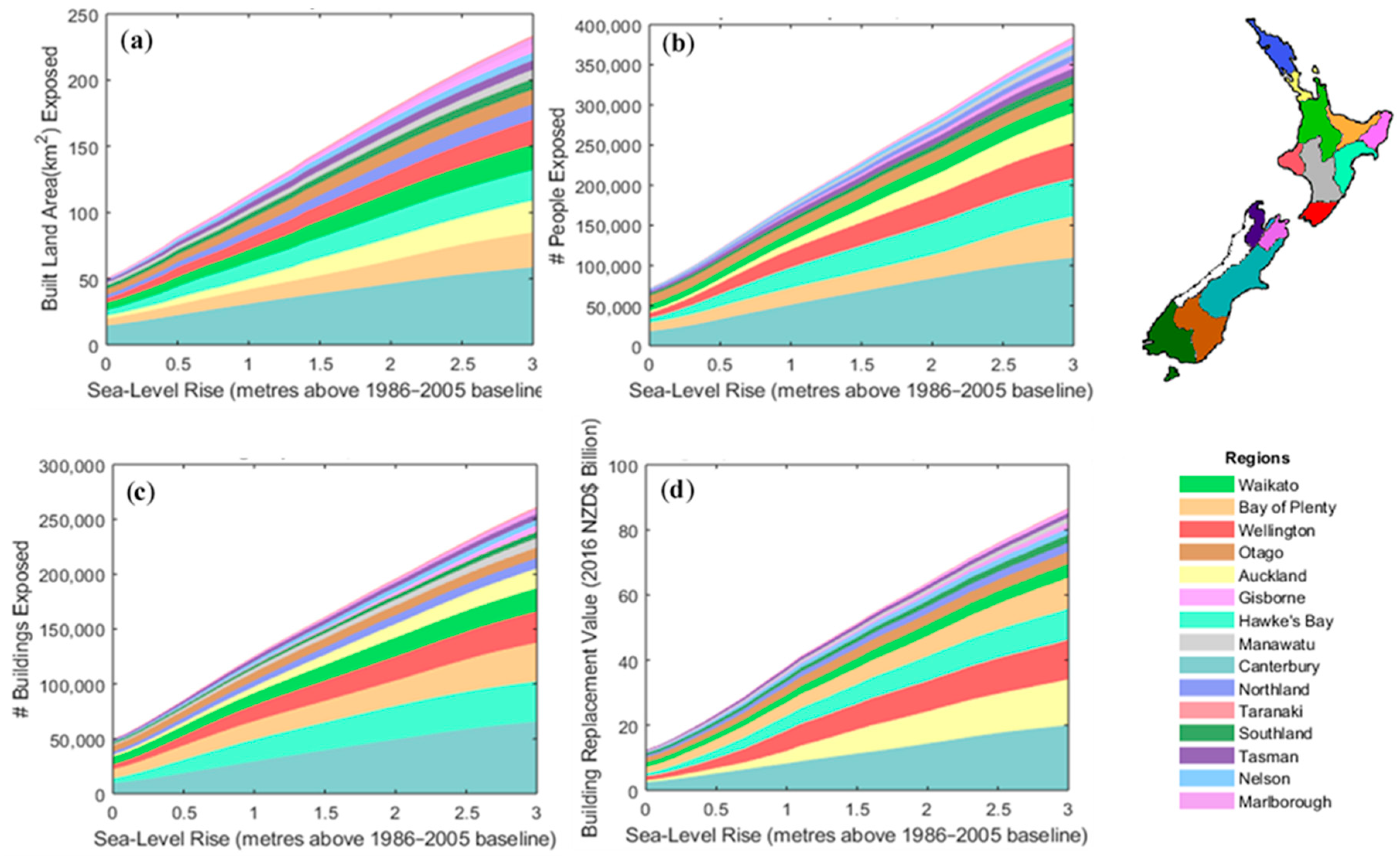
Table S5. The West Coast region is not included in the plots due the absence of LiDAR DEMs.
3.1. National ESL100 Elevations
ESL
100 elevations for the New Zealand coastline are estimated to range between 1.4 m and 4.2 m (
Figure 3,
Table S6). Since storm-surges are relatively small in New Zealand [
24], the spatial pattern of ESL
100 elevation is influenced mainly by the tidal range and wave exposure. Lower ESL
100 elevations of <2 m above MSL occur within estuaries, wave-sheltered embayed coastlines such as the Waikato’s east coast and micro-tidal coastlines within Cook Strait (Wellington Region) and Marlborough Sounds (Marlborough Region). Conversely, the nearby Nelson region adjacent to Marlborough has relatively low wave exposure but higher ESL
100 elevations caused by the largest tides in New Zealand [
29]. ESL
100 elevations are also larger along New Zealand’s west coast due to larger tidal ranges combined with higher wave energy from swells originating in the Southern Ocean [
38]. On the west coast of the South Island, tides are smaller. On the South Island’s east coast, Canterbury is exposed to a high energy southerly wave environment, except in the lee of Banks Peninsula.
3.2. The First Metre of SLR
New Zealand’s land inundation to ESL
100 flooding at MSL
base is 2037 km
2 for areas with LiDAR DEM coverage. This covers 0.8% of New Zealand’s land area. The 50.3 km
2 of built-land at MSL
base (
Figure 1a) exposed includes 49,709 buildings with NZD
$12.4 B replacement value, and a usually-resident population of 72,065, or 1.6% of New Zealand’s 2013 population (
Figure 4b–d). Canterbury region represents 19% and 25% of the exposed building replacement value and population. National building and replacement value exposure increases at an approximately linear rate of 7589 and NZD
$2.5 B respectively for each 0.1 m SLR to 1 m, with exposure doubling by 0.7 m SLR (
Table 3). In Hawke’s Bay, Wellington and Canterbury regions, doubling building and replacement value exposure results in more than 1000 buildings and NZD
$0.35 B value becoming exposed for every 0.1 m SLR increment to 1 m. Additionally, present-day national population exposure almost doubles by 0.7 m SLR, with more than 10,000 people becoming exposed per 0.1 m SLR on average. More than 30% of these people reside in Canterbury, with 10% of the region’s population exposed to ESL
100 flooding by 1 m SLR.
Just over one percent of national road (1414 km) and rail (86.6 km) networks are presently exposed to ESL
100 flooding at MSL
base (
Figure 5a,b). In addition, thirteen of twenty-eight international and domestic airports are exposed (
Figure 5c). National road exposure observes an approximately linear increase of 145 km per 0.1 m SLR to 1 m. This more than doubles the present network exposure from 1414 km to 2856 km. Over the first 1 m of SLR, ESL
100 exposure in Waikato and Canterbury regions will increase by 17.7 km and 28.1 km per 0.1 m SLR, in addition to the 342 km and 243 km exposed at MSL
base respectively. Railway networks are most exposed in regions with high use sea ports, including Auckland, Bay of Plenty and Otago. Railway exposure could more than double to 188.6 km by 1 m SLR.
The national electricity grid supports 122.5 km of transmission lines with 204 structures on land presently exposed to ESL
100 flooding (
Figure 5d,e). ‘Overhead’ lines are predominantly located in Bay of Plenty (30.7 km) and Marlborough (20.5 km), the region servicing the HVDC Inter-Island cable South Island branch. Line exposure could increase by over 60% nationally in response to 1 m SLR. After 1 m SLR, five sites (i.e., substations) servicing the national grid could be potentially exposed to ESL
100 flooding.
Three-waters infrastructure had the highest levels of asset exposure to ESL
100 flooding. National exposure of water nodes exceeds 77,037 at MSL
base, connected to 3179 km of pipelines (
Figure 5i,g). Similar to buildings and other horizontal transport and electricity infrastructure components, the rate of node and pipeline exposure increase is approximately linear with SLR to 1 m. For each 0.1 m SLR increment, national node and pipeline exposure increase by 9504 and 400 km on average, with exposure doubling as SLR exceeds 0.8 m and 0.7 m respectively. In several regions, three-waters node exposure doubles at lower SLR for nodes in Wellington and Nelson at 0.4 m, Auckland and Gisborne at 0.6 m, and pipelines in Nelson at 0.4 m, Wellington at 0.5 m, and Auckland at 0.6 m.
3.3. Beyond the First Metre of SLR
Relative to MSLbase, an almost doubling of flood exposed land covered by LIDAR DEMs occurs as sea-levels rise to 3 m above MSLbase. This is despite a gradual decrease of average incremental exposure rates per 0.1 m SLR. Incremental land area exposure reduces slightly on average from 69.6 km2 every 0.1 m SLR up to 1 m, to 65.2 km2 between 1 m and 2 m SLR, and decreases further to 54.1 km2 between 2 m and 3 m SLR.
Built-land and assets at national-scale exhibit an approximately linear trend of increasing cumulative exposure to ESL
100 flooding as sea-levels rise to 3 m above MSL
base. Within this trend, built-assets exhibit slight variabilities in average incremental exposure per 0.1 m SLR and continues to increase or begin to decrease relative to rates below 1 m SLR (
Table 3). Built-land, railways, transmission lines, electricity structures and building replacement values show slight exposure increases to exposure between 1 m and 2 m SLR, decreasing thereafter. Despite an increasing cumulative exposure trend at national-scale, population and several built-asset types, buildings, roads, three-waters nodes and pipelines show a gradual easing in average incremental exposure rates.
The gradual easing in average incremental exposure for the usually-resident populations and buildings as sea-levels rise beyond 1 m could be attributed to higher rates of commercial, industrial buildings becoming exposed to ESL
100 flooding on higher land. At national-scale, average incremental building replacement value exposure per 0.1 m SLR remains constant up to 2 m SLR (
Table 3). Several populous regions however, show a considerable upturn in average incremental replacement value exposure per 0.1 m SLR at sea-levels above 1 m. In Auckland, New Zealand’s most populous region, average value nearly doubles to NZD
$0.6 B from 1 m to 2 m SLR. At higher sea-levels, such as the Bay of Plenty region, a NZD
$0.11 B increase occurs between 2 m to 3 m SLR. These regions both support major urban areas bordering low-lying estuarine shorelines, suggesting higher value commercial and industrial buildings are becoming increasingly exposed to ESL
100 flooding.
Three-waters infrastructure servicing coastal built-environments observe higher asset exposures for SLR below 1 m (
Table 3). Nationally, three-waters infrastructure networks and buildings connected to their services, exhibit a similar trend whereby a gradual decrease in the rate of incremental exposure occurs above 1 m SLR. Subsequent higher SLR corresponds to an average exposure rate decrease for three-waters node and pipelines by 1905 and 100 km per 0.1 m SLR by 3 m. Despite this trend, Auckland and Bay of Plenty regions show increases in exposed buildings and replacement value between 1 m to 2 m SLR and 2 m to 3 m SLR respectively. At these sea-levels, the potential exposure of higher value commercial and industrial buildings would correspond to three-waters infrastructure exposed to ESL
100 flooding which is highly critical for the social and economic functioning of built-environments.
3.4. Exposure at 3 m SLR: Composite National DEM
The composite national DEM used in the present study, supported ESL
100 flood mapping for SLR projected over century scales by various climate models and RCPs [
8]. National land exposure to flooding reaches 3926 km
2 at 3 m SLR with LiDAR DEM coverage. An additional 2469 km
2 land area is exposed with MERIT DEM coverage. Built-land flood exposure for 3 m SLR extends to 262 km
2, with 28.6 km
2 identified from the satellite-derived DEM. This area includes 289,057 buildings (NZD
$94 B) and a usually-resident population of 423,490. Buildings, their replacement values and usually-resident populations identified from the MERIT DEM represent 9% of the national exposure. This suggests a large proportion of coastal settlements occupied by more than 1000 people are represented by LiDAR DEMs; therefore, providing a reasonable estimate of the national-scale building and usually-resident population ESL
100 flood exposure for SLR < 3 m.
Transport and electricity infrastructure components identified from the MERIT DEM form between 21% and 26% of their national ESL100 flood exposure at 3 m SLR. Network components such as roads, railways, transmission lines and their support structures extend well beyond coastal towns and cities, and are represented by the MERIT DEM in rural areas. At 3 m SLR, 7194 km and 519 km of roads and railways respectively and 451.6 km of transmission lines are exposed to ESL100 flooding. Three-waters node and pipeline infrastructure components represented by the MERIT DEM respectively form just 5% and 6% of their 360,154 and 15,024 km national exposure at 3 m SLR. This is expected as these components predominantly service coastal settlements represented by LiDAR DEMs.
4. Discussion
Global SLR projected over the next century, with its widening uncertainty, will exacerbate built-environment exposure to ESL flooding. In New Zealand, there is already considerable built-land, asset and population exposure to flooding from an ESL
100 event at present-day MSL, which will only increase with SLR. Based on various climate models and RCPs, New Zealand’s MSL is projected to rise between 0.55–1.36 m over the next 100 years [
21]. This SLR range will drive substantial increases in coastal flood event frequencies over the next 100 years, and within the next few decades at relatively low SLR in some locations [
2,
3,
4,
5,
39].
In New Zealand, national exposure of building (including replacement values and usually-resident populations), transport (roads and railways) and three-waters (nodes and pipelines) infrastructure components to ESL
100 flooding doubles with less than 1 m SLR. This is consistent with global scale studies that predict large increases in built-asset and population exposure to SLR over this century [
9,
10,
11,
40,
41,
42]. At regional levels, already high exposure or infrastructure network components including ‘three-waters’ nodes and pipelines to ESL
100 flooding doubles before reaching a 0.5 m SLR. These modest rises in sea-level will cause more frequent ESL flooding exposure that regularly disrupt or reduce infrastructure service levels within built-areas [
43]. This will require adaptation decisions by property owners and communities to proactively manage and plan for the rising and more frequent socio-economic impacts from coastal flooding and SLR.
We found the vertical accuracy of available DEMs limited a consistent national-scale exposure analysis of future ESL
100 flooding. The centimetre-scale vertical resolution of LiDAR data versus metre-scale satellite-derived DEMs, supported more detailed mapping and evaluation of built-asset exposure to ESL
100 flooding and SLR. Our results support findings of [
10], that found improved sub-metre DEM accuracy led to a tripling in the calculated global population exposure to SLR by the year 2100. An advantage of our study was available high-resolution LiDAR DEMs for 40% of New Zealand’s coastline, representing most coastal settlements and urban areas of >1000 people. This enabled differences in ESL
100 flooding exposure to be resolved at 0.1 m SLR increments. Despite significant recent improvements in the vertical accuracy of global satellite DEMs, their relatively lower resolution allows to resolve only large SLR projections over future centuries. In New Zealand, satellite DEMs with at least >2 m vertical accuracy covers the remaining 60% of coastal land where no LiDAR DEMs are available. In the present study, we limited the assessment of ESL
100 flooding exposure to ≤3 m SLR for these areas. For many countries, application of coarser DEMs is inevitable in national-scale exposure assessments but our work shows that substantial improvements can be gained from investment in high-resolution topographic data.
Large uncertainty in projected SLR over the latter part of this century and beyond creates difficulties for investigating and managing coastal flooding impacts on built-environments. Statutes and strategies for managing SLR impacts for prescribed years (e.g., 2100) encounter large SLR ranges coinciding with designated risk interventions, for example, 0.55–1.36 m SLR projections by 2120 for New Zealand. In these situations, applying management interventions too early or too late can be managed using a dynamic adaptive policy pathways (DAPP) approach, where coastal flood exposure or impact indicators trigger adaptive actions ahead of adaptation thresholds [
6,
7,
44]. Identification of coastal flooding adaptation thresholds and triggers over decades and centuries in response to SLR, requires detailed information on the location and timing of flooding and socio-economic impacts for present and future environments [
44,
45,
46,
47]. Applying 0.1 m SLR increments in coastal flood exposure assessments using high-resolution topographic data identifies the spatial variability of present built-asset exposure on temporal scales representing decadal change in SLR and thus included within a DAPP pathway. The timing of these SLR increments can be obtained from projected SLR rates [
3,
5].
National-scale adaptation strategies for future coastal flooding need to consider subnational-scale exposure profiles for increasing increments of SLR. In the present study, we investigated regional built-land and asset exposure to inform a national-scale assessment. There were notable inter-regional differences and differences between the regional and national analyses. At national-scale, an approximately linear trend of increasing built-land and asset exposure is observed as sea-levels rise. However, regions with a high number of built-assets on low-lying coastal land exhibit rapid exposure increases with an only modest SLR, such as Hawke’s Bay, Wellington and Canterbury. In other regions like Auckland and Bay of Plenty where built-assets were located further above sea level due to steeper topography, building and replacement value incremental exposure rates accelerated between 1 m to 2 m and 2 m to 3 m SLR respectively. However, built-assets in most regions, and nationally, will experience their highest average incremental exposure rates below 1 m SLR. This supports the findings of [
3] that coastal adaptation planning and action at all-scales is urgently required to avoid the consequences of deeper and more frequent flooding with rising sea levels.
While this study delivers a first assessment of built-environment exposure to ESLs and SLR in New Zealand, information on social and economic impacts and criticality of built-assets is not provided. Several national- and continental-scale flood impact assessments represent built-environments as continuous land cover maps of simplified built-asset typologies for applying economic vulnerability functions [
36,
48,
49,
50]. Our asset-level approach enabled exposure metrics to be aggregated at scales consistent with local authority decision-making. However, incomplete and inconsistent asset-level attribute information across multiple built-asset typologies limits a detailed spatio-temporal impact analysis. A focus on developing reliable asset-level datasets, coupled with nationally coordinated LiDAR acquisition on low-lying coastal land will considerably improve national-scale assessments of socio-economic impacts arising from built-environment exposure to ESLs and SLR.
5. Conclusions
This study presents a first national-scale assessment of New Zealand’s present and future built-environment exposure to coastal flooding from 100-year extreme sea-levels (ESL100) and SLR. The RiskScape framework was used to identify the flooding exposure of built-land and assets including buildings, transport, electricity, and three-waters infrastructure. The framework used a composite national DEM of high-resolution LiDAR and lower-resolution satellite topographic data. Built-land and asset exposure to flooding was quantified using LiDAR DEMs for present-day MSL and for 0.1 m sea-level increments up to 3 m SLR above present. For the satellite DEM, exposure assessment was limited to a single ≤3 m SLR elevation due to the lower vertical resolution.
We investigated regional built-land and asset ESL100 flooding exposure to inform the national-scale assessment. National exposure to ESL100 flooding doubles with less than 1 m SLR, an observation consistent with global-scale studies on coastal flooding exposure over the next century. Notable inter-regional differences and differences between regional and national exposure trends are observed. An approximately linear trend of increasing built-land and asset exposure occurs in response to SLR at a national-scale. Regions with a high number of built-assets on low-lying coastal land experience rapid increases in exposure at relatively low SLR elevations expected in future decades. This emphasises that national-scale adaptation strategies for future coastal flooding and sea-level rise need flexibility to consider regional and local exposure rates and must facilitate local adaptation planning.
The application of small, regular 0.1 m increments of SLR provides the required resolution to detect variable rates in the magnitude and potential timing (i.e., decadal scale) of future flooding exposure when coupled with SLR projections. This assessment methodology is only possible with high-resolution topographic data, such as LiDAR, and reduces the underestimates that are implicit when using satellite-derived DEMs. Higher resolution built-environment exposure data will facilitate adaptation planning processes by informing adaptation thresholds to be avoided and triggers to begin adaptation actions. Substantial amounts of built-land and assets are already exposed to ESL100 flooding exposure and SLR will drive rapid flooding frequency increases in these areas. This indicates an urgent need for adaptation planning and action to mitigate future socio-economic impacts.


