Urban Vitality, Urban Form, and Land Use: Their Relations within a Geographical Boundary for Walkers

Abstract

The aim of this study was to exmine the influence of combined urban form and land use on the vibrancy in urban areas within a geographical boundary for walkers. A geographical boundary is defined as a block group surrounded by expressways and arterials, based on findings in previous studies. Spatial regression was performed with mobile signal data representing the degree of vitality within the defined areal unit as a dependent variable, and explanatory variables measured by urban form hierarchy were used to consider both natural and built environments. The outcome helps comprehend the physical and functional forms of vibrant neighborhood environments. The result implies the importance of highly desirable features for walking- or transit-friendly neighborhoods. It also indicates the right combination of land uses needed to support the daily lives of local residents: little lost space, short blocks, well-connected streets, short distances to transit stations, and proximity to essential facilities. This study suggests a new way of defining a spatial unit for vitality analysis and shows the critical roles of both natural and built environments in activating local vitality. These findings establish the groundwork for designing better neighborhoods, especially for an area composed of local streets and collector roads.

1. Introduction

Urban vitality is an ideal concept suggested by Jane Jacobs, a prominent urbanist. The aim of using this concept is to improve the quality of citizen life, creating livable and active local environments. In her book, Jane Jacobs specified how to design urban environments to create a vibrant city [1]. She emphasized several requirements for revitalizing urban areas, which included a mixed pattern of land use with two or more uses, small blocks, high enough density that it sufficiently attracts people, buildings of diverse ages, ease of accessibility to public facilities, and control of border vacuums such as large roadways [1]. These requirements are closely connected to walking-friendly environments because the vitality theory is focused on fostering human-scaled environments. Other influential urbanists have also stressed the importance of urban vitality and proposed urban environments that improve the capability to promote the vibrancy of cities to stop auto-oriented development [2,3,4,5]. Their arguments for urban vitality have served as theoretical guidelines and inspired the realm of urban planning and design to this day.

In this context, understanding the actual influences of urban environments on urban vitality has been a major issue for the design of vibrant and livable cities, and also to improve the quality of personal life from the viewpoint of urban management. There have been many attempts to discover the relationship between vitality and urban environments in the academic domain. However, empirical studies for their relationship have only lately progressed because of the difficulty of measuring the degree of urban vitality across a wide area. Researchers regarded the degree of urban vitality as the number of people being active [1,3,5] and measured its degree in various ways. Some studies examined the factors boosting urban vitality using pedestrian count data [6,7,8,9,10,11,12,13,14,15]. Mobile phone data has recently received substantial attention and is regarded as an excellent measure for representing the degree of urban vitality [16]. Multiple researchers have tried to evaluate which urban environments make a city vibrant using mobile phone data [17,18,19,20,21,22]. The results of previous studies generally reached consensus on Jane Jacobs’s theory that mixed use, block size, density, access to public transit, and border vacuums have significant effects on vitality.

However, the past studies have two limitations on (i) defining a geographical boundary so that it captures the localized characteristics of urban form and land use that affect urban vitality and (ii) testing influential variables on vitality considering urban form hierarchy. As for the first limitation on geographical boundaries, previous studies might not adequately consider a geographically appropriate scale to capture the localized characteristics that affect urban vitality. The previous studies have examined vitality at various scales (e.g., location, street, grids, census tracts, and administrative districts), but these scales were based on the ease of data processing. If the scale is too small, some attributes of urban environments are unobserved in spite of their significant impact. Conversely, when the scale is too large, attribute measures may be too aggregated to reflect their characteristics adequately. For example, if a residential area was measured together with commercial or industrial uses in a large-scale geographical boundary that is not a neighborhood boundary of residents, the functional role of residences in a certain area may be distorted. This scale issue has been discussed in the field of geography, referred to as the modifiable areal unit problem (MAUP) [23,24]. The MAUP has also been dealt with in studies on the relationship between urban environments and the travel and activities of various citizens [25,26,27,28]. These studies support the importance of defining a proper geographic areal unit for confirming the different outcomes by areal unit type and size. Zhang and Kukadia [28] suggest the approach of using the behavioral characteristics of people to define a reasonable scale when studying the effect of urban environments.

Among the variables used for urban environments, the most commonly referenced categorizations for measuring built environments are the “3Ds”: density, diversity, and design [29] and the “5Ds”: density, diversity, design, distance to transit, and destination accessibility [6]. These categorizations are very reasonable for finding the factors most influential for travel behavior, but have a slight deficiency for systematically reflecting the hierarchy of urban form; the “3Ds” and “5Ds” focus only on built environments. In this regard, this study borrowed the urban morphology concept to measure urban environments including both natural and built environments. The urban morphology concept divides urban form into four elements: natural context, street system, plot system, and building system [30]. These elements of the urban form govern the quality of citizens’ daily lives by determining available spaces, their density, and accessibility. Moreover, urban form combined with land use has an important role in deciding the magnitude of activities. Land use can be defined using various classification criteria and refers to a series of functional attributes of different spaces such as commercial, residential, and industrial [31]. Both urban form and land use are decided in the first step of urban planning and are very hard to transform after first being developed because of laws and regulations, the long periods needed to change, and high construction costs.

In this respect, the aim of this study is to figure out the relationship between urban form, land use, and urban vitality based on the urban form hierarchy. Seoul in South Korea was selected as a study site. Service population data estimated based on mobile phone signals was used as a proxy measure of urban vitality. The urban form and land use were measured in four categories and within a defined areal unit able to precisely capture the specifications of urban environments related to urban vitality. Diverse geographical data related to the physical and functional form of urban area was utilized to measure the characteristics of urban form and land use. The results of this study can provide further thought and information for a straightforward application of urban-planning procedure for a vibrant, sustainable city.

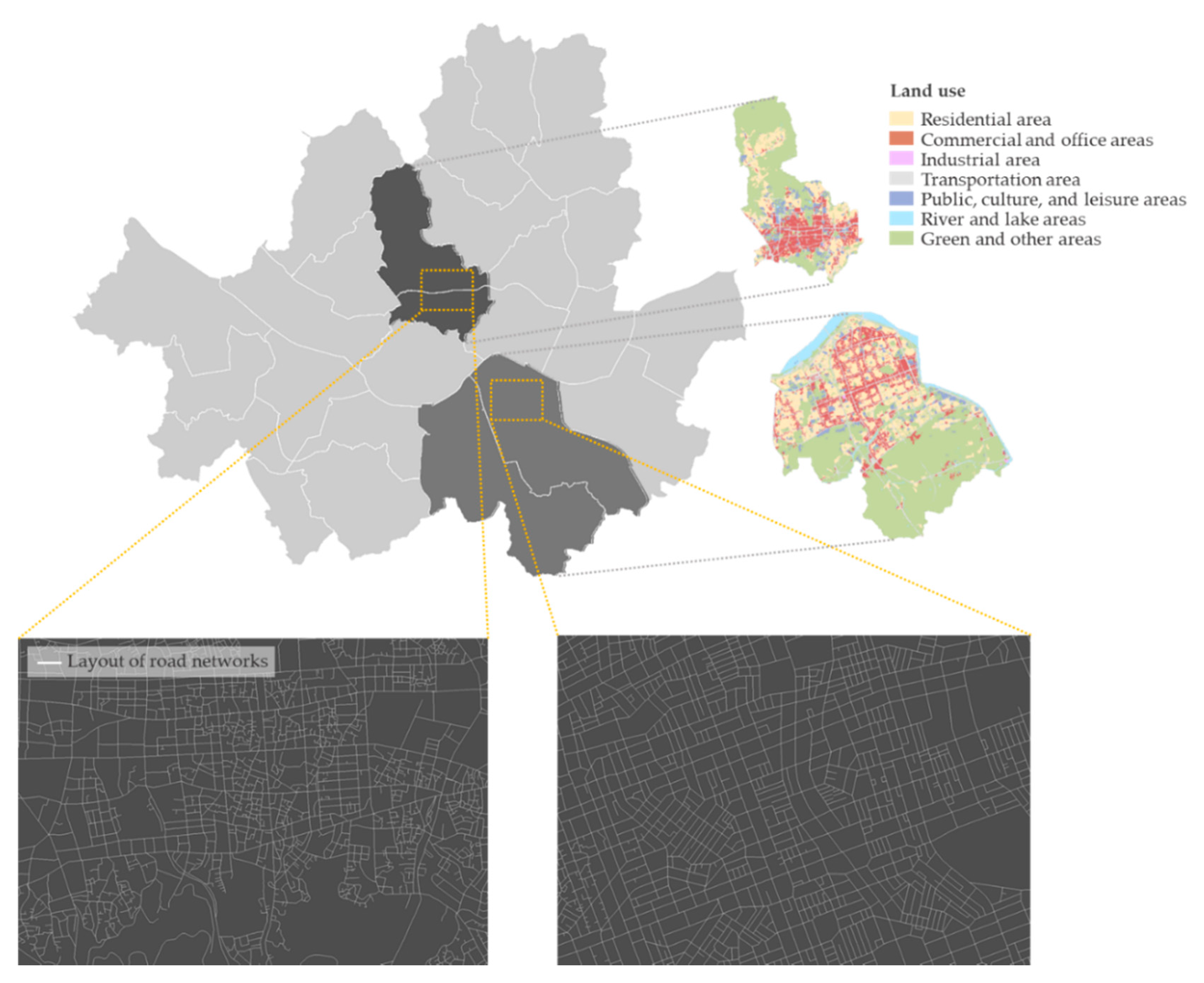
2. Study Site and Data Sources

The geographical scope of this study includes four districts in Seoul Metropolitan City. Seoul is the largest city in South Korea, and has a high level of development, mixed land uses, and transit-rich neighborhoods. As the city’s importance in the economic and cultural sphere has grown, more people visit Seoul for individual purposes such as business, education, and leisure. Almost 11.3 million people occupy Seoul in the daytime, while the number of registered residents is 10 million people (in 2020) [32].

Figure 1 shows where the study sites are. The two northern districts (Jongno-gu and Jung-gu) have old business districts, and the two southern districts (Seocho-gu and Gangnam-gu) have newer business districts. They include some residential regions and also some of the most crowded regions in the daytime that are considered central business districts (CBDs). In addition, they have a similar population density: 8.2 thousand people/km² for the northern two districts and 8.8 thousand people/km² for the southern districts [32]. These four districts were selected as study sites because they have similar functions within Seoul but have contrasting urban forms. Figure 1 displays the road network forms of the northern and southern districts—while the southern districts have a grid-like layout, the road networks in the northern districts combine various layouts such as curves and dead ends.

To measure urban environments for this study, a GIS (Geographical Information System) database was built by collecting a variety of spatial data. The South Korean government provides transportation and urban data with different coordinate systems among various agencies. For this study, the geographic data was compiled and mapped to a common coordinate system. The database includes information about the service population [32], transit station locations [32], a road name address map [33], building layout data [34], a land use zoning map [34], and an administrative boundaries map [34].

3. Methodology

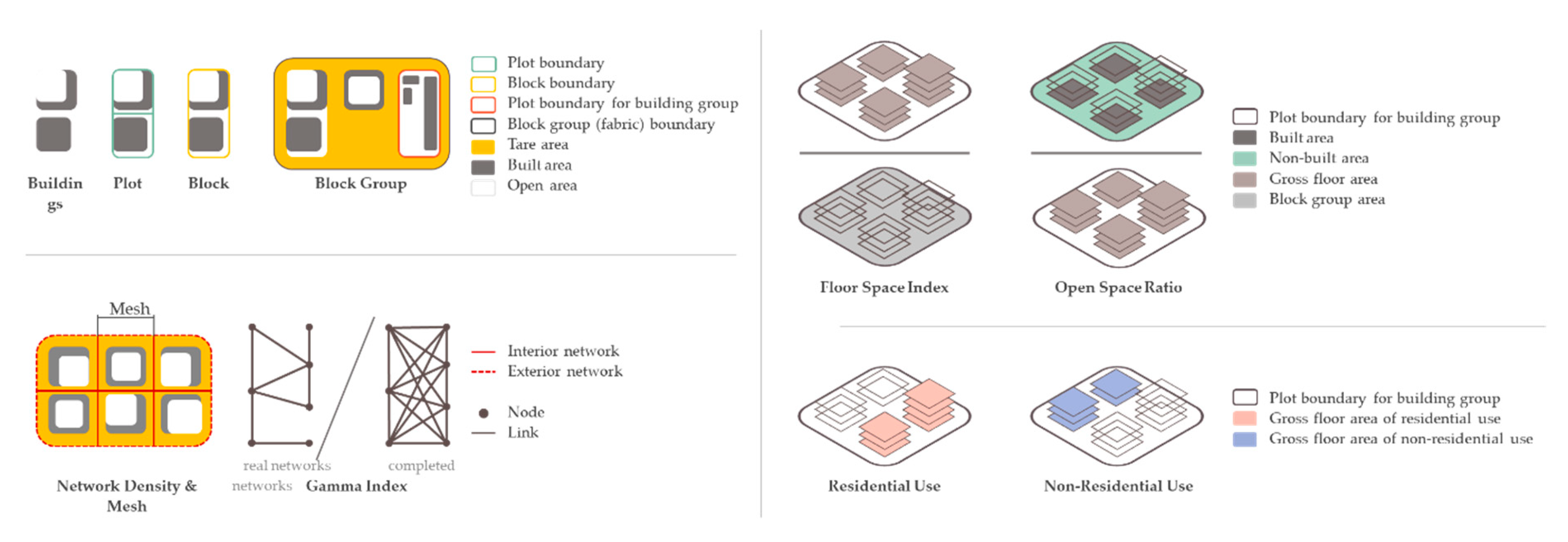
3.1. Geographic Scale to Capture Urban Form and Land Use Factors

To capture urban form factors influencing vitality, the author defined a geographic scale after referring to the literature on urban environments and walking behavior. The reason for considering walking is that theories related to urban vitality are rooted in creating walking-friendly environments within walking boundaries [1,2,3,4,5]. They emphasized the human-scaled design of urban environments. The grounds for defining the geographical scale are listed below:

• Expressways and arterials are the roadway functional classifications that mainly serve for the mobility of vehicles, not the actual activities of people.
• Massive single-use roadways play the role of borders in cities [1].
• The roadways (including arterials) where many vehicles pass at high speed decrease the frequency of people crossings [35].
• Livable and safe communities can be provided by narrow streets, not wide arterials [36].
• Public transit (subway and bus) is taken as one of the major transportation modes. Their routes pass mostly on arterials. In Seoul, subways account for 39.9% of transport, buses 25.1%, vehicles 24.4%, taxis 6.5%, and all others 4.1% [32].

Based on these five grounds, the de-facto demarcation for walking—the areal unit—was defined using the road hierarchy. The defined areal unit (i.e., geographical scale) is a block group surrounded by expressways and arterials—also referred to as “fabric” in urban planning. Among the designated groups, the groups composed of only water and green spaces through which walkers cannot pass were excluded. The final number of block groups was 217 samples, that is, 85 samples for the northern districts and 132 samples for the southern districts (see Figure 2).

3.2. Measuring Urban Form and Land Use Variables

With the defined areal unit being the block group, the study variables were measured for analysis. The service population data were used as a dependent variable considering the daily numbers from 6 a.m. to 9 p.m. on all weekdays (Monday to Friday) in April 2018. This data was acquired from the Seoul Open Data Plaza [32]. The Seoul Metropolitan Government provides this data, which is estimated based on the number of mobile phone signals every day. The month of April was selected as the temporal scope of this study because it has the least bias from national holidays in South Korea. The statistics included those of both local residents (i.e., mostly Koreans) and visiting foreigners in order to measure the totality of people staying within the study site.

The explanatory variables are a combination of urban form and land use. For this study, the concept of urban morphology [30] was borrowed to categorize the variables and the categorization included four elements: natural context, network form (street and transit), plot form, and building form and land use. After referring to the literature related to urban form, explanatory variables in the categories were measured [31,37]. The variables related to land use were included in the same category with building form because the land use variable was measured using gross floor areas of buildings to capture land-use intensity, not just the surface area typical of individual land use.

The natural context is the first element of urban form, which includes natural environments, and significantly affects the organization of other urban form elements and the configurations of infrastructure and human settlement in a city [30]. In this category, there were two variables: tare space and slope of land. The tare area indicates the share of space unused or unavailable for people’s activities in the block groups, such as green belts and land with water surfaces. The slope of land in each block group was included in the natural context in the form of average incline.

The second category (street system) is a layout of the street networks in a city, which forms cities with diverse street types, shapes, and widths, and also with various ways of joining streets. Citizens travel, access places, and interact with neighboring environments on streets. Jane Jacobs and Bill Hillier, who are prominent urbanists, accentuate the crucial role of streets for livable and vigorous cities [1,38]. At the block group (i.e., fabric) level, which is the areal unit for this study, the network density was measured as the length of street networks per area of block group [37]. Mesh was also calculated as the reciprocal of the network density multiplied by 2 [37]. The mesh means the average distance between streets in a square grid of a block group. The gamma index is a measure of connectivity based on graph theory, which compares the number of real links and maximum links that can be connected by real nodes [31]. A value close to one indicates a well-connected street network. For public transit networks, the number of subway station entrances and bus stops were counted and divided by the area of the block group to express density.

The plot system determines the detailed demarcation of areas within a layout of street networks. The number and shape of plots per street block affect the arrangement of the building system. The variable “building entrance density” evaluates the accessibility of buildings by people. The share of plot area for building groups represents the ratio of plots for building groups out of all plots for buildings in individual block groups. The building group indicates the multiple buildings located in one plot area for single-use. The ratio of the plot for a building group to the built area signifies the degree of building density at the plot level. If the share of plots for building groups is close to zero, it means fewer building groups. In contrast, a value close to “1” indicates a higher proportion of building groups. The average plot area and the number of plots per square kilometer were also included in the list of variables.

The variables in the building form and land use category provide information about the three-dimensional spaces available and the land-use intensity. The floor space index (FSI) expresses building intensity in individual block groups, and the open space ratio (OSR) indicates the amount of non-built area in a block group at ground level [37]. The surface area of individual land use zones is generally utilized as a measure, but it has limits for representing land-use intensity. For this study, the gross floor area was measured by each type of purpose (i.e., building use) to observe both pattern and intensity of land use in localized areas. These play critical roles in estimating the magnitude of urban activities. The types of building use include residential, neighborhood commercial, general and central commercial, office, and education and welfare. The balance indices were computed using the gross floor area by building use to compare the intensities of each land use. Residential use was set as a base indicator and the balanced level with non-residential use was measured using the equation of balance index [39]. In addition to the above variables, the type of district and area of a block group unit were included as control variables. More details of all variables are tabulated in

Table 1. Description and summary statistics of variables.

Variables	Description	Unit	Mean	Std. Dev
Dependent Variable
service population	number of local population and foreigners	thousand people	161.800	124.556
Explanatory Variable
Natural Context
tare area	unused or unavailable areas for people	km2/km2	0.306	0.158
slope	average elevation of land	degree	3.549	4.304
Network Form
street network density	density of street networks	km/km2	0.020	0.012
mesh	average length between streets in a square grid	km/km2	141.547	124.130
gamma index	connectivity of street networks		0.294	0.129
subway station entrance density	station entrances per 1 km2	number/km2	7.591	11.456
bus stop density	bus stops per 1 km2	number/km2	32.170	20.588
Plot form
building entrance density	building entrances per 1 km2	number/km2	1264.031	1255.164
share of plot for building group	share of plot area for building group against all plots	km2/km2	0.057	0.144
plot for building group / built area	ratio of plot area for building groups against built area of all buildings	km2/km2	2.427	2.944
average plot area	average area of plots	km2	0.002	0.004
number of plots per km2	number of plots per 1 km2	number/km2	2673.673	2859.738
Building Form and Land Use
floor area ratio	building intensity	km2/km2	1.590	1.128
open space ratio	spaciousness	km2/km2	2.201	11.518
residential buildings	gross floor area of residential buildings	number	0.456	0.288
balance index 1	balance index between gross floor areas of neighborhood commercial and residential buildings	index	0.461	0.305
balance index 2	balance index between gross floor areas of non-daily commercial and residential buildings	index	0.173	0.240
balance index 3	balance index between gross floor areas of office and residential buildings	index	0.111	0.171
balance index 4	balance index between gross floor areas of education and welfare and residential buildings	index	0.163	0.239
Control Variables
area of block group	block group area	km2	0.523	0.940
type of district	north districts = 1 south districts = 0	dummy variable	0.392	0.489

, and their measuring methods are described in Appendix A (

Table A1. Measurement methods of explanatory variables.

Variables	Measurement
Natural Context
tare area	tare area/BGA
slope	average elevation of land
Network Form
street network density	$\frac{\mathrm{length}\mathrm{of}\mathrm{interior}\mathrm{networks}+\mathrm{length}\mathrm{of}\mathrm{exterior}\mathrm{networks}/2}{\mathrm{BGA}}$
mesh	2/street network density
gamma index	number of links/3(number of nodes—2)
subway station entrance density	number of subway station entrances/BGA
bus stop density	number of bus stops/BGA
Plot Form
building entrance density	number of building entrances/BGA
share of plot for building group	areas of plot area for building groups/areas of all plots
plot for building group / built area	areas of plots for building groups/built areas of all buildings
average plot area	sum of all areas of plots/number of plots
number of plots per km2	number of plots BGA
Building Form and Land Use
floor area ratio	gross floor area (GFA)/BGA
open space ratio	(1—built areas)/floor area ratio
residential buildings	GFA of residential buildings
balance index 1	$1-\left|\frac{\mathrm{GFA}\mathrm{of}\mathrm{residential}\mathrm{use}-\mathrm{GFA}\mathrm{of}\mathrm{non}-\mathrm{residential}\mathrm{use}}{\mathrm{GFA}\mathrm{of}\mathrm{residential}\mathrm{use}+\mathrm{GFA}\mathrm{of}\mathrm{non}-\mathrm{residential}\mathrm{use}}\right|$
balance index 2
balance index 3
balance index 4
Control Variables
area of block group	block group area (BGA)
type of district	dummy variable

and Figure A1).

3.3. Specification of Spatial Regression

The Global Moran’s I test was performed to observe the inherent nature of spatially collected data (i.e., the spatial autocorrelation). This test is a classic measure that examines the presence of the spatial autocorrelation phenomenon in the data. This phenomenon signifies interactions among nearby observations over space. When the null hypothesis is a random distribution of data over space, a Moran’s I index close to “1” indicates that the data is spatially clustered; an index close to “−1” indicates that dissimilar observations in the data are next to each other with a dispersion shape [40]. The service population data was tested, and the result confirmed the presence of the spatial autocorrelation phenomenon in the data. On the basis of the test results (Moran’s Index of 0.184 and p-value of 0.000), the null hypothesis was rejected.

Considering the result of the Global Moran’s I test, the spatial regression modeling was adopted for the analysis to handle the spatial autocorrelation in the data. The spatial regression model is a universal econometric method that adds a spatial weighting matrix to the general regression function [41,42]. The specification of the spatial regression model is given below.

$$Y=\rho WY+X\beta +\epsilon , \epsilon ={\left(I-\lambda W\right)}^{-1}\mu , when \mu ~N\left(0,\Omega \right)$$

(1)

where $Y$ is a dependent variable with the form of a vector, and $X$ is explanatory variables with a matrix form. Here, $W$ is a spatial weighting matrix and $\beta$ is the vector of estimated coefficients of explanatory variables. The terms $\epsilon$ and $\mu$ are unobserved error terms, and $\rho$ and $\lambda$ are coefficients for the spatial autoregressive structure.

The above function becomes a spatial autoregressive model (SAR) when $\lambda$ is zero, and becomes the spatial error model (SEM) when $\rho$ is zero. Both models deal with the spatial dependence of the data. The SEM does not offer information on spatial spillover towards nearby areas, while the SAR provides the magnitude of spillover effects [43].

In the present study, a spatial weighting matrix, W, was calculated based on the distances between observations: $w_{ij}=1/d_{ij}$(if $i\ne j \mathrm{and}{d}_{ij}<D)$ and $w_{ij}=0$ (if $i\ne j\mathrm{and}{d}_{ij}\ge D, or \mathrm{i}=\mathrm{j})$. Moran’s I Indices were computed for a series of distances to find a fiducial distance, D, which indicates the neighborhood influence boundary. The fiducial point was defined as the distance with maximum autocorrelation: 2 km.

Before modeling the final model, the Lagrange Multiplier (LM) test was used to decide on a proper model between SAR and SEM for the data [42,44]. In the test, the spatial regression model is compared to the ordinary least square model to validate the performance of the spatial model. The null hypothesis is that $\rho$ or $\lambda$ is zero; the model with zero of $\rho$ or $\lambda$ is an ordinary least square model [44]. If the LM test result supports acceptance of the null hypothesis, it means the ordinary least square model is appropriate for this data. All analyses were conducted in R using the “spdep” and “spatialreg” packages [45,46].

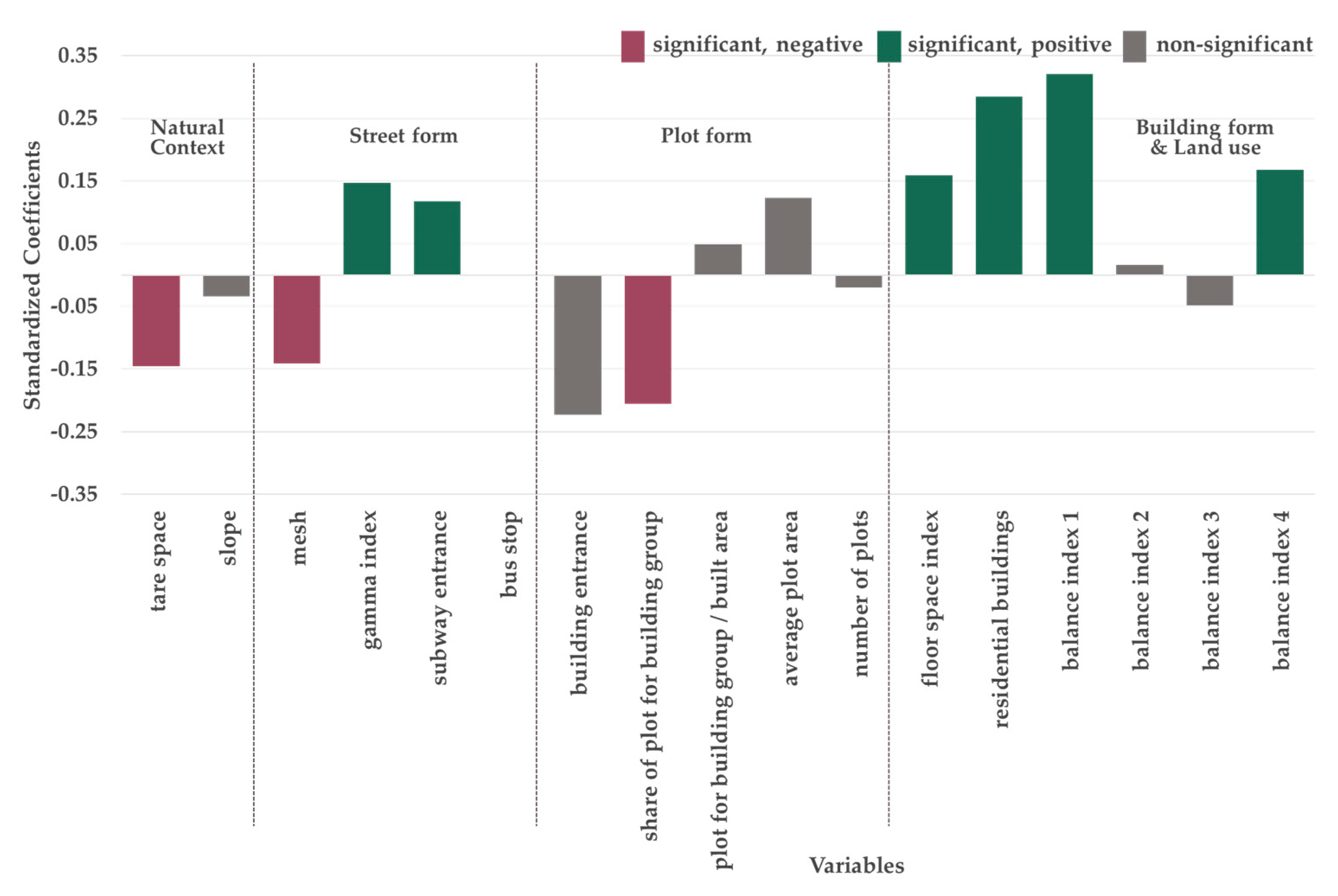
4. Interpretation of Results

The Lagrange multiplier (LM) test guides selection of the better spatial regression model for the data (between the spatial autoregressive model and the spatial error model). The results of the LM test indicated that the spatial autoregressive model was better than the spatial error model at explaining the relationships between the urban environments and vitality (see

Table 2. Results of the Lagrange Multiplier test.

Model	Statistics	p-Value	Acceptance
Spatial error model	4.792	0.029	Reject
Spatial autoregressive model	10.311	0.001	Reject
Robust Spatial error model	0.221	0.639	Accept
Robust Spatial autoregressive model	5.739	0.017	Reject

).

Table 3. Results of spatial autoregressive modeling.

	Moran’s I of Residuals	Log-Likelihood		Adj. R2	AICc
OLS	0.055 (0.000)			0.363	2683.7
Spatialautoregressive model	0.012 (0.247)	−1316.189		0.443	2676.4
Variables	Coef.	Std. Coef.	Std. error	z-value	p > |z|
Natural Context
Tare **	−129.930	−0.146	61.188	−2.123	0.034
slope	−1.094	−0.034	2.794	−0.392	0.695
Network form
Mesh *	−0.159	−0.141	0.092	−1.721	0.085
gamma index **	159.510	0.147	70.838	2.252	0.024
subway entrance density *	1.428	0.117	0.796	1.794	0.073
bus stop density	−0.016	−0.002	0.395	−0.039	0.969
Plot form
building entrance density	−0.025	−0.223	0.016	−1.558	0.119
share of plot for building group **	−200.020	−0.206	75.329	−2.655	0.00
plot for building group/built area	2.349	0.049	3.286	0.715	0.475
average plot area	4268.100	0.123	3048.600	1.400	0.162
number of plots per km2	−0.001	−0.020	0.007	−0.137	0.891
Building form and land use
floor area ratio **	19.739	0.159	8.371	2.358	0.018
residential buildings ***	55.269	0.284	12.187	4.535	0.000
balance index 1 ***	149.560	0.320	33.530	4.460	0.000
balance index 2	7.903	0.016	35.691	0.221	0.825
balance index 3	−29.137	−0.049	29.625	−0.984	0.325
balance index 4 **	74.420	0.168	30.377	2.450	0.014
Control variables
area of unit ***	41.126	0.276	12.790	3.216	0.001
type of district	21.656	0.076	23.715	0.913	0.361
intercept	−5.518		49.227	−0.112	0.911
$\rho$***	0.392		0.109	3.592	0.000

Significance levels: *** p < 0.01, ** p < 0.05, * p < 0.1.

shows all estimates of the final model using the spatial autoregressive model and the model performance indicators of the OLS model. Moran’s I test of residuals confirms that the final model using spatial regression solves the problem of spatial autocorrelation in the data. Moreover, adjusted R² and the Akaike Information Criterion (AIC) values indicate better performance of the spatial regression model than of the OLS model.

The statistically significant $\rho$ in the spatial autoregressive model indicates the existence of spatial dependence in the data across the study site. This means that the urban environments within a certain boundary not only determine the vitality of the area, but that they also exert an influence on surrounding areas. This may be a natural outcome when considering various spatial interactions by people within communities.

In the final model, some explanatory variables were excluded because of correlated relationships with other variables. The excluded variables are network density and open space ratio. The network density has a correlation coefficient of -0.667 with the mesh. The open space ratio correlates with the tare area with a correlation coefficient of 0.324. The modeling result shows ten explanatory variables with statistical significance. The standardized coefficients were also provided to compare the effect size of variables on the same scale. Figure 3 shows the standardized coefficients of all variables in a graph form. The absolute value of the standardized coefficient is the largest in the balance index between residential and neighborhood commercial uses, with a value of 0.320. Several variables in the plot form, and building form and land use, also have larger standardized coefficients (> 0.200).

In the natural context category, the tare area, which represents the portion of areas unused or unavailable for activities in the daily life of the people, has a negative coefficient in the model. This indicates that a large tare area impedes vibrant activities of the people. This result implies that highly developed two-dimensional space promotes vitality.

In the network form category, the variables of mesh, gamma index, and subway entrance density are statistically significant. Their estimated outcome corresponds to the requirements for walkability and accessibility in the concept of Transit-Oriented Development (TOD), which involves pedestrian-friendly and connected network design. Mesh means an average distance between roads, with the same meaning as an average block length. The coefficient of the mesh variable is −0.175, indicating that blocks with longer length hinder vitality. This result is comparable with the arguments about whether smaller or shorter blocks provide positive influences on improving walkability and transit use [44]. Another network variable, the gamma index, is an indicator for rating network connectivity that is calculated using the number of nodes and links within a street layout. The coefficient of the gamma index has a positive value, indicating that well-connected streets promote activities of the people. The result implies that the southern districts composed of more well-connected streets may induce more vibrant activity than the northern districts do when the conditions of other environments are the same. The importance of well-connected streets frequently appears in a guideline for walking-friendly environments. It has the effect of dispersing vehicle traffic and decreasing distances and elapsed times to destinations [47]. Last, the subway entrance density represents the level of accessibility to a transit station. Higher accessibility to transit stations increases the ability of people to travel to participate in various activities. The coefficient of subway entrance density is a positive value, which may be a natural result, in that the modal share of public transit is high in Seoul. This estimated result verifies the importance of transit to improve vitality in the city.

The share of plot areas for building groups is the only statistically significant variable in the plot form category. The building group indicates the multiple buildings constructed in one plot for single-use. The standardized coefficient of this variable has a negative value and a size of −0.206 (much larger than the others). This indicates that a large-scale building group for single-use interrupts people’s vibrant activities. The negative effect of building groups was validated in a previous study that investigated the relationship between walking activity and neighborhood environments. The work of Sung et al. [13] confirmed that large-scale building development discourages walking activity and increases the likelihood of driving. Such large plot design is widespread in residential districts in South Korea, in the form of apartment complexes. This housing type makes a gated community and semi-public space, limiting full public access [48]. This may hinder interactions between neighboring areas and penetrability into the district and, consequently, improvement of neighborhood vitality.

Among the explanatory variables of building form and land use, the floor area ratio, residential buildings, and two balance indices for land use were statistically significant. The floor area ratio is the ratio of the total gross floor area to the area of the block group. This is measured to represent the usable space available from a three-dimensional perspective. The estimated coefficient of the floor area ratio indicates that a higher floor area ratio connects to better environments for vibrant activities because expanded usable spaces provide diverse content for people. The estimated coefficients of the balance indices of land use show how to design neighboring areas, especially for residents. This is closely connected to proper combinations of land uses for people’s daily lives. The balance indices of neighborhood commerce and education and welfare with residential uses have statistically significant coefficients with positive values. The outcome of balance indices enhances the basic attribute of urban planning. A high degree of balance between neighborhood commerce or education and welfare with residence is an essential requirement for improving the quality of people’s daily lives and promoting vibrancy in the city.

5. Conclusions and Discussion

This study was intended to examine the influence of combined urban form and land use on the vibrancy in urban areas. In this study, their relationships were explored from the urban morphological perspective. Four districts of Seoul were tested, and service population data estimated using mobile phone signals were used as a proxy measure of urban vitality. Variables able to explain urban environments were measured using a variety of spatial data and categorized into four groups based on the concept of urban morphology: natural context, network form (street and transit), plot form, and building form and land use. The present study defined an areal unit as a block group surrounded by expressways and arterials to reveal the urban environments affecting vitality at a proper geographical scale, considering a de-facto boundary for walkers. The relationship between urban environments and vitality was estimated using a spatial regression model to deal with the spatial autocorrelation phenomenon in the spatially collected data.

The outcome of this study helps to comprehend the physical and functional forms of vibrant neighborhood environments. The result of statistically significant spatial dependency showed that urban environments in a certain area interact with urban environments in the surrounding areas, and, thereby, influence activities in the surrounding areas as well as in the given area. The estimated coefficients of variables show a close connection between pedestrian- and transit-oriented design requirements. Notably, the results are consistent with highly desirable features for walking-friendly neighborhoods: little lost space, short blocks, well-connected streets, short distances to transit stations, and proximity to facilities supportive of people’s daily lives. These findings demonstrate the arguments of Jane Jacobs and support previous studies highlighting the significance of pedestrian- and transit-oriented design for creating vibrant neighborhoods.

In addition, the estimated coefficients of the balance indices between land use types enhance the importance of the right combination of land uses for the lives of local residents. In a transit-oriented city with a functionally severed structure like Seoul, the residential regions require a close arrangement of neighborhood commercial, education, and welfare facilities such as grocery stores, clinics, daily sports clubs, schools, and public offices, which are closely related to people’s ordinary lives. This balanced land use arrangement induces vibrant activities by guaranteeing essential amenities for citizens in the neighboring areas.

This study is meaningful in suggesting a new way of defining the areal unit for analyzing urban activity from the urban vitality perspective and for econometrically verifying the suggestions of old but valuable theories about vibrant cities. The modeling result offers an opportunity to understand numerically the environmental elements needed for vitality in relation to the urban form hierarchy. It tells us the importance of walking-friendly and functionally balanced neighborhoods to improve vitality. This study establishes groundwork upon which to plan urban environments to foster neighborhood vibrancy, and can especially assist in designing areas composed of local streets and collector roads. For practical planning, the findings of this study can provide a pedestrian-oriented guideline to site planning of new development and redevelopment zones. Furthermore, the findings of this study towards vibrant neighborhoods support the smart city initiatives in that they highlight assuring sustainable transportation modes and accessibility to amenities closely related to livability [49,50]. However, because this study is based on the quantitative data measured by information technology, the qualitative evaluation of vitality in local areas by citizens who live in those areas could not be explained, which may be a critical determinant of the level of vitality. Further study should proceed with consideration of the qualitative feature of vitality.

References

1. Jacobs, J. The Death and Life of Great American Cities; Vintage Books: New York, NY, USA, 1961. [Google Scholar]
2. Gehl, J. Life between Buildings: Using Public Space; Island Press: Washington, DC, USA, 2011. [Google Scholar]
3. Lynch, K. Good City Form; MIT Press: Cambridge, MA, USA, 1984. [Google Scholar]
4. Montgomery, J. Editorial urban vitality and the culture of cities. Plan. Pract. Res. 1995, 10, 101–110. [Google Scholar] [CrossRef]
5. Montgomery, J. Making a city: Urbanity, vitality and urban design. J. Urban Des. 1998, 3, 93–116. [Google Scholar] [CrossRef]
6. Cervero, R.; Sarmiento, O.L.; Jacoby, E.; Gomez, L.F.; Neiman, A. Influences of built environments on walking and cycling: Lessons from Bogotá. Int. J. Sustain. Transp. 2009, 3, 203–226. [Google Scholar] [CrossRef]
7. Kang, C.-D. Measuring the effects of street network configurations on walking in Seoul, Korea. Cities 2017, 71, 30–40. [Google Scholar] [CrossRef]
8. Kim, S.; Park, S.; Jang, K. Spatially-varying effects of built environment determinants on walking. Transp. Res. Part A Policy Pract. 2019, 123, 188–199. [Google Scholar] [CrossRef]
9. Kim, S.; Park, S.; Lee, J.S. Meso-or micro-scale? Environmental factors influencing pedestrian satisfaction. Transp. Res. Part D Transp. Environ. 2014, 30, 10–20. [Google Scholar] [CrossRef]
10. Park, S.; Deakin, E.; Jang, K. Can Good Walkability Expand the Size of Transit-Oriented Developments? Transp. Res. Rec. 2015, 2519, 157–164. [Google Scholar] [CrossRef]
11. Saelens, B.E.; Handy, S.L. Built environment correlates of walking: A review. Med. Sci. Sports Exerc. 2008, 40 (Suppl. 7), S550. [Google Scholar] [CrossRef] [PubMed] [Green Version]
12. Sung, H.; Lee, S. Residential built environment and walking activity: Empirical evidence of Jane Jacobs’ urban vitality. Transp. Res. Part D Transp. Environ. 2015, 41, 318–329. [Google Scholar] [CrossRef]
13. Sung, H.; Lee, S.; Cheon, S. Operationalizing Jane Jacobs’s urban design theory: Empirical verification from the great city of Seoul, Korea. J. Plan. Educ. Res. 2015, 35, 117–130. [Google Scholar] [CrossRef]
14. Sung, H.; Lee, S.; Jung, S. Identifying the relationship between the objectively measured built environment and walking activity in the high-density and transit-oriented city, Seoul, Korea. Environ. Plan. B Plan. Des. 2014, 41, 637–660. [Google Scholar] [CrossRef]
15. Sung, H.-G.; Go, D.-H.; Choi, C.G. Evidence of Jacobs’s street life in the great Seoul city: Identifying the association of physical environment with walking activity on streets. Cities 2013, 35, 164–173. [Google Scholar] [CrossRef]
16. Ratti, C.; Frenchman, D.; Pulselli, R.M.; Williams, S. Mobile landscapes: Using location data from cell phones for urban analysis. Environ. Plan. B Plan. Des. 2006, 33, 727–748. [Google Scholar] [CrossRef]
17. De Nadai, M.; Staiano, J.; Larcher, R.; Sebe, N.; Quercia, D.; Lepri, B. The death and life of great Italian cities: A mobile phone data perspective. In Proceedings of the 25th international conference on world wide web, Montreal, QC, Canada, 11–15 April 2016; pp. 413–423. [Google Scholar]
18. Delclòs-Alió, X.; Gutiérrez, A.; Miralles-Guasch, C. The urban vitality conditions of Jane Jacobs in Barcelona: Residential and smartphone-based tracking measurements of the built environment in a Mediterranean metropolis. Cities 2019, 86, 220–228. [Google Scholar] [CrossRef]
19. Jacobs-Crisioni, C.; Rietveld, P.; Koomen, E.; Tranos, E. Evaluating the impact of land-use density and mix on spatiotemporal urban activity patterns: An exploratory study using mobile phone data. Environ. Plan. A 2014, 46, 2769–2785. [Google Scholar] [CrossRef]
20. Jin, X.; Long, Y.; Sun, W.; Lu, Y.; Yang, X.; Tang, J. Evaluating cities’ vitality and identifying ghost cities in China with emerging geographical data. Cities 2017, 63, 98–109. [Google Scholar] [CrossRef]
21. Wu, W.; Niu, X. Influence of Built Environment on Urban Vitality: Case Study of Shanghai Using Mobile Phone Location Data. J. Urban Plan. Dev. 2019, 145, 04019007. [Google Scholar] [CrossRef]
22. Ye, Y.; Li, D.; Liu, X. How block density and typology affect urban vitality: An exploratory analysis in Shenzhen, China. Urban Geogr. 2018, 39, 631–652. [Google Scholar] [CrossRef]
23. Fotheringham, A.S.; Wong, D.W. The modifiable areal unit problem in multivariate statistical analysis. Environ. Plan. A 1991, 23, 1025–1044. [Google Scholar] [CrossRef]
24. Jelinski, D.E.; Wu, J. The modifiable areal unit problem and implications for landscape ecology. Landsc. Ecol. 1996, 11, 129–140. [Google Scholar] [CrossRef]
25. Clark, A.; Scott, D. Understanding the impact of the modifiable areal unit problem on the relationship between active travel and the built environment. Urban Stud. 2014, 51, 284–299. [Google Scholar] [CrossRef]
26. Houston, D. Implications of the modifiable areal unit problem for assessing built environment correlates of moderate and vigorous physical activity. Appl. Geogr. 2014, 50, 40–47. [Google Scholar] [CrossRef]
27. Yang, L.; Hu, L.; Wang, Z. The built environment and trip chaining behaviour revisited: The joint effects of the modifiable areal unit problem and tour purpose. Urban Stud. 2019, 56, 795–817. [Google Scholar] [CrossRef]
28. Zhang, M.; Kukadia, N. Metrics of urban form and the modifiable areal unit problem. Transp. Res. Rec. 2005, 1902, 71–79. [Google Scholar] [CrossRef]
29. Cervero, R.; Kockelman, K. Travel demand and the 3Ds: Density, diversity, and design. Transp. Res. Part D Transp. Environ. 1997, 2, 199–219. [Google Scholar] [CrossRef]
30. Oliveira, V. Urban Morphology: An Introduction to the Study of the Physical Form of Cities; Springer: Berlin/Heidelberg, Germany, 2016. [Google Scholar]
31. Rodrigue, J.-P.; Comtois, C.; Slack, B. The Geography of Transport Systems; Routledge: England, UK, 2016. [Google Scholar]
32. Seoul Open Data Plaza. Available online: https://data.seoul.go.kr (accessed on 20 November 2020).
33. Road Name Address. Available online: https://www.juso.go.kr (accessed on 20 November 2020).
34. Korea National Spatial Data Infrastructure Portal. Available online: http://www.nsdi.go.kr (accessed on 20 November 2020).
35. Donald, A.; Gerson, M.S.; Lintell, M. Livable Streets; University of California Press: Berkeley, CA, USA, 1981. [Google Scholar]
36. Rosales, J. Road Diet Handbook: Setting Trends for Livable Streets; Parsons Brinckerhoff: New York, NY, USA, 2006. [Google Scholar]
37. Berghauser-Pont, M.; Haupt, P. Spacematrix: Space, Density and Urban Form; NAi Publishers: Rotterdam, The Netherlands, 2010. [Google Scholar]
38. Hillier, B. Spatial sustainability in cities: Organic patterns and sustainable forms. In Proceedings of the 7th International Space Syntax Symposium, Stockholm, Sweden, 8–11 June 2009. [Google Scholar]
39. Cervero, R.; Duncan, M. Walking, bicycling, and urban landscapes: Evidence from the San Francisco Bay Area. Am. J. Public Health 2003, 93, 1478–1483. [Google Scholar] [CrossRef] [PubMed]
40. Kelejian, H.H.; Prucha, I.R. On the asymptotic distribution of the Moran I test statistic with applications. J. Econ. 2001, 104, 219–257. [Google Scholar] [CrossRef] [Green Version]
41. Anselin, L. Spatial Econometrics: A Companion to Theoretical Econometrics; Blackwell Publishing Ltd.: Hoboken, NJ, USA, 2001. [Google Scholar]
42. Anselin, L. Spatial Econometrics: Methods and Models; Springer Science & Business Media: Berlin/Heidelberg, Germany, 2013; Volume 4. [Google Scholar]
43. Vega, S.H.; Elhorst, J.P. On spatial econometric models, spillover effects, and W. In Proceedings of the 53rd ERSA Congress, Palermo, Italy, 27–31 August 2013. [Google Scholar]
44. Anselin, L. Lagrange multiplier test diagnostics for spatial dependence and spatial heterogeneity. Geogr. Anal. 1988, 20, 1–17. [Google Scholar] [CrossRef]
45. Bivand, R.; Bernat, A.; Carvalho, M.; Chun, Y.; Dormann, C.; Dray, S.; Halbersma, R.; Lewin-Koh, N.; Ma, J.; Millo, G. The spdep package. Compr. R Arch. Netw. Version 2005, 5–83. [Google Scholar]
46. Bivand, R.; Pebesma, J.; Gómez-Rubio, V.; Pebesma, E. Applied Spatial Data Analysis with R; Springer: New York, NY, USA, 2008. [Google Scholar]
47. Ewing, R.; Bartholomew, K. Pedestrian & Transit-Oriented Design; Urban Land Institute: Washington, DC, USA, 2013. [Google Scholar]
48. Joo, S.-M.; Kim, J.-Y. A Study on Street Vitality of Two Different Types of Superblocks—With a case of Yeoksam 2-dong, Seoul. J. Archit. Inst. Korea Plan. Des. 2019, 35, 71–82. [Google Scholar]
49. Chourabi, H.; Nam, T.; Walker, S.; Gil-Garcia, J.R.; Mellouli, S.; Nahon, K.; Pardo, T.A.; Scholl, H.J. Understanding smart cities: An integrative framework. In Proceedings of the 2012 45th Hawaii international conference on system sciences, Maui, HI, USA, 4–7 January 2012; pp. 2289–2297. [Google Scholar]
50. Neirotti, P.; De Marco, A.; Cagliano, A.C.; Mangano, G.; Scorrano, F. Current trends in Smart City initiatives: Some stylised facts. Cities 2014, 38, 25–36. [Google Scholar] [CrossRef] [Green Version]
Figure 1. Study site and its land use and layout of street networks.
Sustainability 12 10633 g001
Figure 2. Geographical boundaries as designed for analysis.
Sustainability 12 10633 g002
Figure 3. Estimated coefficients of spatial autoregressive modeling.
Sustainability 12 10633 g003