Comparison of Different Monetization Methods in LCA: A Review

Abstract

Different LCA methods based on monetization of environmental impacts are available. Therefore, relevant monetization methods, namely Ecovalue12, Stepwise2006, LIME3, Ecotax, EVR, EPS, the Environmental Prices Handbook, Trucost and the MMG-Method were compared quantitatively and qualitatively, yielding results for 18 impact categories. Monetary factors for the same impact category range mostly between two orders of magnitude for the assessed methods, with some exceptions (e.g., mineral resources with five orders of magnitude). Among the qualitative criteria, per capita income, and thus the geographical reference, has the biggest influence on the obtained monetary factors. When the monetization methods were applied to the domestic yearly environmental damages of an average EU citizen, their monetary values ranged between 7941.13 €/capita (Ecotax) and 224.06 €/capita (LIME3). The prioritization of impact categories varies: Stepwise and Ecovalue assign over 50% of the per capita damages to climate change, while EPS and LIME3 assign around 50% to mineral and fossil resource use. Choices regarding the geographical reference, the Areas of Protection included, cost perspectives and the approach to discounting strongly affect the magnitude of the monetary factors. Therefore, practitioners should choose monetization methods with care and potentially apply varying methods to assess the robustness of their results.

1. Introduction

Human activities lead to manifold impacts on the environment. Without a unique metric, it is difficult to decide which of the impacts are most severe and thus need to be prioritized to reduce overall environmental impact. Monetization of environmental impacts is one solution to this problem. The monetization of environmental impacts is the conversion of environmental impacts caused by releases of environmentally harmful substances or the use of natural resources to monetary units.

Today, monetization of environmental impacts is mostly used in such contexts as (environmentally extended or social) cost-benefit-analysis (CBA) [1].

While monetization can also facilitate the creation of markets for so-far non-marketed goods (e.g., for emission permits or payments for ecosystem services), this article focuses on determining economic value of impacts caused by environmental releases, leading to associated costs to society. Distinguishing between these kind of market prices of goods and economic values of impacts is important [2,3] and is sometimes confused (e.g., when scholars just use the emission permit price of CO₂ to determine the associated damages of the emission as in [4,5]). Leaving aside this theoretically inconsistent approach, different ways to determine costs for the reduction or exhaustion of natural goods (such as biodiversity or biotic and abiotic natural resources) are possible, notably the marginal damages of an emission to nature or as a second-best approach the marginal costs of reaching a political target (e.g., the Paris agreement) [6]. When determining marginal damage costs, a range of different approaches exist to convert biophysical flows into monetary units namely:

• The market price approach,
• The revealed preference approach,
• The stated preference approach.

Which approach is used depends on whether the flows are measured through their connection to a marketed good (market price approach), to their connection to a surrogate good (revealed preference) or whether the Willingness to Pay (WTP) is measured through surveys (e.g., contingent valuation) [6].

Monetizing life cycle assessment (LCA) results is one form of weighting in LCA [7] that enables the handling of trade-offs between impact categories. As Life Cycle Assessment (LCA) is one of the recommended management tools to quantify environmental impacts along the life cycle, there are movements to connect LCA with CBA [8] or to derive a single score through monetized LCA results as an index for ecological performance [9]. The advantage of monetized environmental impacts is that they can overcome the problem of trade-offs between the many impact categories an LCA usually analyzes. However, since it usually delivers a single score, it currently only conforms to the ISO standard (14040/44) [10,11] if it is used for internal communication in an organization. Since 1992, approaches to monetize LCA results have been developed, among which the first method was the Environmental Priority Strategies (EPS) [12]. Since then, many other methods have evolved, including updates of existing methods, such as the LIME method in Japan that has been updated three times [13,14,15], or the method by Vogtländer et al. [16] (Environmental-Costs/Value-Ratio- hereafter EVR) that has been updated several times. Thus, the questions arise: how do these methods compare, and does it matter which method is applied?

Up to now, six peer reviewed reviews address monetization in LCA, which differ in their scope and core conclusions. The first review by Finnveden [17] evaluated the EPS method and compared it to an approach developed in the first funding period of the External Costs of Energy (ExternE) project. Several calculation errors in the EPS method were found. The next review also by Finnveden et al. [18] concluded that if LCA results are monetized, all impact categories should be monetized using the same cost perspective (defined as monetization approaches such at abatement costs, damage costs or societal WTP). Based on this assumption, the Ecotax approach was developed that monetizes all impacts via environmental taxes. The next review by Ferreira et al. [19] compared EVR, Stepwise and Ecovalue08 quantitatively, identifying Ecovalue08 and EVR as having the lowest and highest monetary factors, respectively. However, they did not provide an in-depth analysis on the reasons why the results differ, but highlighted that there is research needed to compare the underlying mechanisms in more detail. The most comprehensive review up to date was published by Pizzol et al. [20]. It classified the different methods according to their monetization approach and their impact categories. It developed a scoring system to evaluate the different monetization approaches. They concluded that LIME2 and Stepwise are the most suitable methods because they provide explicit weighting between areas of protection (AoP) that are congruent to the impact endpoints in environmental LCA. They also perform a small quantitative comparison of different LCA monetization methods on a per-impact category basis, but with limited coverage of impact categories.

Two more recent reviews focused on the monetization of the impact category climate change [21] and monetization in LCA in the building sector [22]. Durão et al. [22] state that only mid-point monetization is compatible with EPDs, because they provide monetary factors that are compatible with the required CML-midpoint categories that must be included in an EPD. Dong et al. [21] identified that the emission values for global warming have similar values but still there is a spread of one to two orders of magnitude for the monetary valuation of CO₂. They identify which damages and endpoints are integrated into the damage assessment, which was also done in this review but for more impact categories.

While also being as comprehensive as Pizzol et al. [20], the novelty of this review is that a link between the monetary damage factors and the valuation of the respective AoP is established when the documentation allows. Through this analysis, it is possible to obtain an overview, which AoPs are linked to which impact categories and how the respective monetary valuation of the AoP is connected to the monetary factor for the emission. Further, we integrate the new LIME update, the new EPS update, the Trucost method, the MMG update and the EVR update, which have not been included in any review up to date.

Inspired by the review of different monetary values for GHG by Bachmann [3], monetary factors from the analyzed methods for the different impact category indicators are confronted, after adjusting them to allow for direct comparison. The comparison is done quantitatively and qualitatively and evaluates which kind of damages are included in the different monetization methods. Further, we analyze the distribution of the monetary values per impact category. Thus, the aim of this review is to perform a detailed quantitative and qualitative comparison of the currently used monetization methods in LCA on a general and on a per impact category basis, which has not been done in any review so far. Further, we establish a link between qualitative and quantitative differences of the applied methods. Based on this approach, the aim of the paper is to:

• Provide an overview of existing and relevant monetization methods in LCA;
• Determine criteria which influence the magnitude of the costs and why;
• Assess how the different monetization methods value and prioritize environmental damages of an average EU citizen;
• Identify overarching weaknesses within the impact categories;
• Outline overarching challenges to establish a roadmap according to which monetization in LCA can develop towards a consensus.

The paper is structured as follows: in the upcoming section, the qualitative and quantitative evaluation methods are described. Then the results are presented. First, the general qualitative results (Section 3.1) and then the quantitative results (Section 3.2) are displayed. The results chapter ends with Section 3.3 that integrates the qualitative and the quantitative findings per impact category. In Section 4 and Section 5, the results are discussed and a conclusion is drawn.

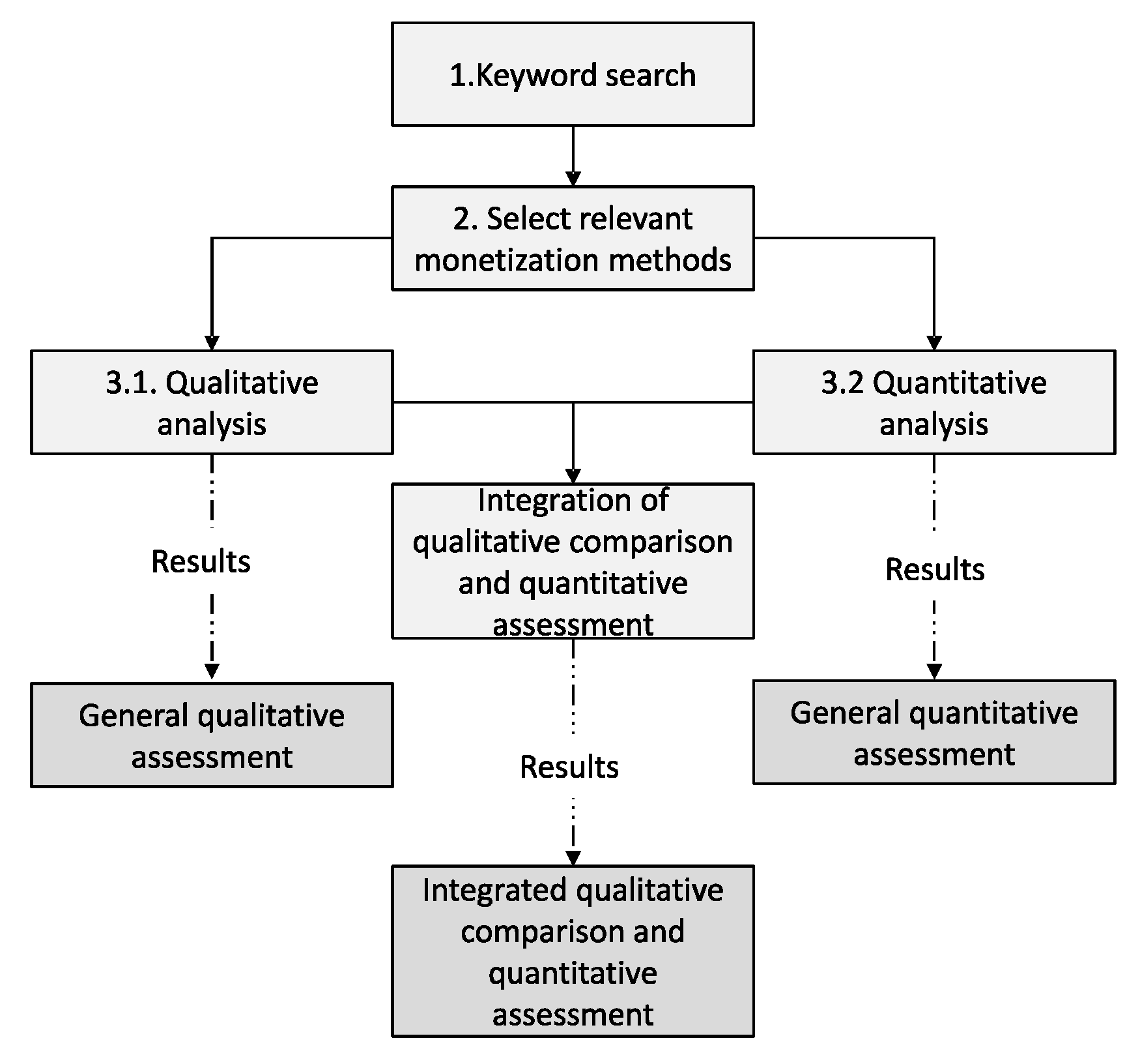
2. Materials and Methods

In order to assess the different methods and their monetary units, four steps were taken (see Figure 1).

First, a key word search was performed in Scopus and Web of Science. Fifty articles were extracted that contain the words “LCA” AND “monetization” OR “LCA” AND “monetary valuation” published after 2013. In this year the last comprehensive literature review was closed [20].

In the second step, relevant papers describing the monetization methods were identified by screening all the extracted abstracts and papers. In those papers, more references that are relevant were mentioned so that 100 studies were studied in total. We classified the studies into case studies (43 papers), methodological publications (38 papers) and discussion/review papers (19 papers). Based on the discussion and review papers, an evaluation scheme for the qualitative assessment was developed. Nine relevant monetization methods were identified that fulfilled the following three criteria:

• They have an associated peer-reviewed case study released after 2012;
• They are the latest method update of the respective method (e.g., because LIME 3 was included, LIME2 and LIME were not);
• They have a strong connection to LCA and provide monetary factor(s) per impact category.

Only one of the identified methods (Trucost) is a pure weighting method; the other methods have a coupled life cycle impact assessment and weighting. In the third step, the quantitative and qualitative comparison was performed. It was limited to those impact categories for which at least two of the nine monetization methods provide monetary values. The qualitative comparison was based on criteria deemed significant (see Section 2.1 for the specific criteria). They were adopted from review and discussion papers like [3,20,21], but were also based on environmental economic foundations [6,23].

The final step is the integration of the qualitative comparison and the quantitative assessment. The question that was guiding us in this final step is: can the quantitative differences be explained by the qualitative differences?

2.1. Qualitative Comparison

The criteria for the qualitative comparison are:

• The cost perspective and the type of market used when assessing damages (see Figure 2),
• The included AoPs,
• The use of equity weighting,
• The used discount rate,
• Whether marginal or non-marginal impacts are valued,
• The handling of uncertainty.

These aspects are assessed per method and per impact category. In the following, these criteria are explained in more detail.

Cost perspectives: The cost perspectives were classified as specified in Bachmann [6], i.e., damage costs based on individual’s WTP or proxies thereof (here referred to as societies WTP), and abatement costs (tier 1). Damage costs are further distinguished according to the kind of market on which the monetary values are determined. The damage-oriented cost perspectives can be further classified into the market price approach, revealed preference approach or stated preference approach (tier 2). The classification of the cost perspectives can be seen in Figure 2.

Another important distinction usually made in environmental economics is the difference between willingness to pay (WTP) and willingness to accept (WTA). The WTA is up to seven times higher [24] than the WTP, due to the income effect [23,24], bad-deal aversion [25], the endowment effect or study design. While the difference between WTP and WTA has been studied intensively, there is a strong tendency in environmental economics to use WTP instead of WTA [23], especially because WTA often yields protest votes and higher values. Therefore, we pay specific attention to whether WTP or WTA is determined by the monetary valuation methods.

Moreover, all monetary valuation methods (irrespective of WTP and WTA) have been criticized for being wealth sensitive (obtaining higher results for wealthier people). This is an aspect that we analyze through (i) the covered geographical scope and (ii) the use (or not) of equity weighting.

AoPs: The different impact categories in LCA have a link to an AoP. For ReCiPe, for example, these AoPs are human health, resource scarcity and ecosystem quality [26]. LIME 3, by contrast, distinguishes four AoPs: human health, social assets, biodiversity and primary production [27]. Further AoPs distinguished include the built environment or labor productivity [28]. The methods establish different links and therefore include different damages: for example, some include the cause-effect chain from POCP (Photochemical Ozone Creation) to material corrosion and some do not. For the purpose of this study, we distinguish the following AoPs: human health, agricultural production, ecosystems, resources (abiotic and biotic resource production), working capacity, buildings and materials and human wellbeing (by which we mean the enjoyment of scenic beauty and positive aspects of enjoying an unpolluted environment beyond health). Following the links between impact categories and AoPs from ReCiPe (figure 1.1 in the ReCiPe report) and the Environmental Prices Handbook (figure 5 and table 25 in the Environmental Prices Handbook) [26,29], we determine which AoPs are included in which impact category of those methods that have the damage cost perspective. If a link is outlined in the Environmental Prices Handbook, it does not necessarily mean that it is quantified separately in its monetization (e.g., the Environmental Prices Handbook connects climate change impacts to human health ecosystems and resources, but uses the abatement costs to derive its monetary factor for climate change). Further, we compare how the AoPs for human health and ecosystems are monetized.

Equity weighting: Equity weighting is the practice in which environmental prices are corrected for their wealth sensitivity [30]. Depending on the used factors, environmental damages that make poorer people suffer can be scaled in a way that they are as valuable (or in extreme cases even more valuable) than damages to richer people. Generally, it is an ethical decision whether equity weighting is used or not. We assess it as a criterion, because it has an impact on the results, since methods with equity weighting will yield higher results.

Geographical scope: As explained earlier, monetary valuation of environmental damages is often wealth sensitive. In addition, a certain emission may be particularly damaging in a certain area (e.g., since an area is especially species rich and thus more highly valued). For these reasons, the geographical scope is analyzed.

Discounting: Discounting is used in economics to convert future costs into current value. Hellweg et al. [31] discussed discounting in relation to LCA and concluded that LCA impacts should not be discounted. Discounting of values associated with non-marketed goods is a topic which has always been controversial (see particularly the Nordhaus/Stern debate [32,33]). Note that cutting-off impacts that occur after a certain point in the future (e.g., 100 years from now) is also a kind of discounting [3,31]. Without taking a position in this debate, we recognize that a higher discount rate will yield lower results and vice versa. Therefore, we obtain the discount rate to have another criterion for possible differences in the assessment results.

Marginal/non-marginal analysis: Usually, in LCA, potential environmental impacts are assessed due to a small change in emissions (marginal). This is because LCA is usually used to assess environmental impacts of products that only bring about a small change. Since LCA is used more and more to assess bigger objects such as cities [34,35], territories [36] and organizations [37], its impact modelling and associated characterization factors need to be adapted [38,39]. The various impact assessment methods assessed in this review approach this topic differently. The chosen reference point has a significant impact on the assessed damages, which is also influenced by the choice between consequential and attributional LCA. Some methods just take the average damages of all emissions (in a certain impact category) globally; they determine the damages by average damages following this equation:

Average Damages = AD = TD/q,

(1)

where TD stands for total damages, and q for quantity of the respective emission (adapted from [40]). Others assess the damages of a small emission change (in that impact category), the mathematical description of marginal damage is (adapted from [40]):

Marginal Damages = MD = Change in TD/Change in q,

(2)

For some impacts such as climate change or water use, the marginal damages of the environmental impact increase as the background or reference environmental impact level rises. As a result, the marginal damages of those impact categories will be higher than average damages in our analysis. This can be seen in the rising damages for the next unit of CO₂ emissions for nearly all integrated assessment models as temperature increases [41], or through the conclusion that the CO₂-price should rise, because its marginal damages also rise with increasing emissions. Revesz et al. [41] highlight this effect for species richness when they conclude that most integrated assessment models underestimate the damages to ecosystems, since the value of the next species lost rises when species become scarcer as they go extinct. For other impact categories the cause-effect relationship is different and site-dependent, e.g., acidification.

Uncertainty: We analyze whether the methods provide uncertainty factors and which methods they use to determine uncertainty.

2.2. Quantitative Assessment

For the quantitative assessment all monetary units are converted to 2019 €. The conversion was performed according to the guideline of ISO 14008 [42]. First, the monetary values are inflated by the Consumer Price index, and then they are transferred to € by Purchasing Power Parities, where necessary. Some methods do not provide the reference year for the monetary units. Then we assumed that the €-unit was from the respective publication year. The following equation was used to correct for inflation based on [43].

X_t = X_b × CPI_t/CPI_b

(3)

where X_t stands for the currency in the target year, X_b for the currency in the base year and CPI for the Consumer Price Index in the respective years t and b. The values were taken from different statistical offices [44,45,46].

After the correction for inflation, we converted currencies in the following manner:

currency value_target = currency value_original/PPP_original × PPP_target

(4)

while PPP stands for Purchasing Power Parity. PPP_original is the PPP value of the original currency and PPP_target is the PPP of the target currency (in our case €). PPP values were taken from OECD [47].

To compare all methods quantitatively, they need to relate to the same impact category indicator and unit. For some impact categories (e.g., climate change), all monetization methods use the same impact category indicator (CO₂-e), whereas for other impact categories these impact category indicators differ. Thus, the impact category indicators were converted to the same unit according to Owsianiak et al. [48] and Dreyer et al. [49]. First, a unit conversion factor (UCF) to convert unit a to unit b is determined:

UCF_a→b = 1/CF_a→b

(5)

Then the monetary factors are converted to unit b by the following equation:

MF_b = MF_a × UCF_a→b

(6)

MF_b stands for the monetary damage per unit of b, MF_a for the monetary damage per unit of a. CF_a→b stands for the characterization factor for the substance a that characterizes the substance in terms of b (i.e., how much b is as harmful as one unit of a, thus b is the reference impact category indicator). CF_a→b has the unit b/a. UCF_a→b stands for the unit conversion factor from the impact category indicator a to b. The applied CFs and derived UCFs are available in Table S1 in the supplementary material. For LIME3, we had to extract the impact category specific results. We did this using ReCiPe impact assessment for all impact categories except for mineral resources (CML) and water (Ecoscarcity) [50].

Where possible, ReCiPe [26] (Hierarchist perspective) conversion factors were used. For some impact categories other approaches were needed (e.g., USEtox [51], Impact 2002+ [52], methods from the ILCD recommendations for acidification [53] or TRACI [54]), because certain flows were not characterized in ReCiPe. For the impact categories mineral resources, fossil resources and toxicity, a different approach was taken. For mineral resources only antimony was assessed, because several methods did not conduct a characterization step, but just monetized at inventory level. To convert the values of the fossil energy carriers from mass units to energy units, the mass units were multiplied with the heating value from [55]. For the comparison of human toxicity units and for freshwater ecotoxicity, USEtox was used. Moreover, some methods did not provide information to which media the toxic substance was released, so assumptions were necessary. Further, only some impact assessment methods distinguished between cancer and non-cancer effects. In order to reach some comparative results anyway, the following approach was taken: first, the monetary damage per emission were converted to CTUh (Comparative toxic units) cancer or non-cancer. The characterization factors used were USEtox characterization factors and are given in CTUh per kg of emission. These were converted to DALYs (Disability Adjusted Life Years) to obtain a comparable € value per DALY, applying the conversion factors by Huijbregts et al. [56] (one CTUh non-cancer equals to 2.7 DALYs and one CTUh cancer equals to 11.5 DALYs). This yielded the monetary value per DALY. For the methods that provided values for CTUh-cancer and CTUh non-cancer separately, we assessed those values separately.

As a next step, the distribution of the values for the different impact categories were compared. To compare all impact categories with each other, we divided the obtained values per impact category by the mean of the impact category of all analyzed methods and displayed the distribution in a boxplot. To avoid the fact that methods which provide various values have a stronger weight in the mean of the impact category, we calculated an average monetary value for each method and derived the mean based on those average values (e.g., only the central estimate of the Ecovalue method was considered).

Then, we created a ranking of the quantitative results across impact categories (i.e., we assessed how many times a certain method had the highest, second highest value etc.). This enabled us to compare our obtained quantitative results with the formulated hypothesis in the general part to where we expect higher or lower values. This was done using the following formula:

Score for method_x = (∑rank of impact category_y × rank)/(number of impact categories covered)

(7)

Finally, we multiplied the obtained values with European normalization factors for 2010 [57], to see whether the methods obtained similar weighting between midpoints and to determine the extent to which the obtained monetary values differ across impact categories. For mineral and fossil resource use we took global values from [58] and assumed corresponding emissions per capita, as the European values only provided one value for mineral and fossil resources. Further, land use, terrestrial and marine ecotoxicity had to be excluded, because the European normalization did not fit to the impact category indicators we used for the unit conversion.

2.3. Integration of Qualitative Comparison and Quantitative Assessment Per Mid-Point Impact Category

As a final step, the quantitative and qualitative results were compared in detail. We identified the reasons why the values are different and connected our qualitative finding with our quantitative results. The integration of these results has a per impact category focus.

3. Results

In this chapter, the results are presented. Firstly, we describe the results of the qualitative assessment (Section 3.1) and the quantitative assessment (Section 3.2) per monetization method. To interpret the quantitative results, we partially draw on the results from the qualitative assessment. Then the results of the integration of the qualitative comparison are generated and the quantitative assessment is performed on the per impact category basis (Section 3.3).

3.1. Qualitative Criteria Based Assessment

Based on the established criteria in the method section we classify the assessed methods. An overview of all qualitative results is delivered in

Table 1. Overview of methods based on the criteria presented in the method part.

Method	Cost Perspective	AoPs 1	Equity Weighting	Geographical Scope	Discounting	Marginal/non-Marginal	Uncertainty	Associated Publications
Ecovalue12	Damage costs/stated preference and market price	Divers for different impact categories, partially no documentation	Not clearly documented	Sweden	Unclear	Marginal	Provides min and max values	[59,60,61,62,63]
Stepwise 2006	Damage costs/Ability to pay	Human health biodiversity resources	Yes	Global	Unclear	Marginal	Discussed qualitatively	[64,65]
LIME3	Damage costs/stated preference	Human health, social assets (natural resources), terrestrial ecosystems, NPP 1	No	Global with country resolution (G20 countries)	No	Marginal except for climate change	No	[13,27,66,67,68,69]
Ecotax 2006	Societies’ willingness to pay	Not applicable	Not applicable- as it is not connected to an AoP	Sweden	Not applicable	Marginal	Provides min and max values	[18]
EVR (version 1.6)	Abatement costs	Not applicable	Yes but only applicable for human toxicity	Europe Netherlands 2	Not applicable	marginal		[16,70,71]
EPS	Damage costs/mostly market price and revealed preference	Human health, bio productivity, biodiversity, abiotic resources, water, labor productivity	Yes, every human welfare loss is treated as if they were an OECD citizen	Global	0%	average	Provides uncertainty factors	[28]
Environmental Prices	Damage costs and abatement costs	Human health, ecosystems, buildings and materials, resource availability, wellbeing	No (but use only one DALY 1 for all European countries)	Europe	3%	Marginal	High, low and central value (but not for LCA 1 weighting factors)	[29]
MMG-Method	Damage costs abatement costs restoration costs	Human health-, biodiversity, agricultural production, resources	Not explicitly treated-	Europe, Flanders 2, global 2	3%	CO2, POCP 1, Water -marginal, for the other impacts unspecified	Provides a high middle and low estimate	[72,73,74,75]
Trucost	WTP 1 through ecosystem services (market price) or stated preference	Human health, ecosystem services based on de Groot [76], abiotic resources	Yes, DALYS 1 for all people are weighted equally	Global	Yes, but rate is unclear (for human health it is 3% as it is based on [77])	Eutrophication, abiotic resources acidification, smog, toxicity,: marginal, land use: average:	Qualitative description of uncertainty and limitations	[78]

^1. Abbreviations are DALY: disability adjusted life year, AoP: area of protection, POCP: photochemical ozone creation, LCA: Life Cycle Assessment, WTP: willingness to pay, NPP: net-primary production ² These geographical scopes are not considered in the evaluation.

. This result supplements the specific analysis of all impact categories and how they are assessed. In the remaining part of this section, the results for all criteria for the different methods are outlined.

Cost perspective: Most methods use the damage costs as their cost perspective, whereas the EVR uses abatement costs and Ecotax uses societies’ WTP. There are some exceptions to this, for example in the impact category global warming most methods use abatement costs. Even though seven methods mostly use damage costs, they use different approaches and techniques to determine the damages. The damages were determined through the market price approach, through the revealed preference approach (with techniques such as the travel cost method) or through the stated preference approach (with techniques such as choice experiments or contingent valuation). Find more details on the specific impact categories in the integration of the qualitative comparison and the quantitative assessment (Section 3.3). Another finding is that all methods that determine damage costs through contingent valuation use the WTP approach, but no method uses WTA.

AoPs: In the following, we will present the underlying monetary values that the different methods use for the AoPs human health and biodiversity/ecosystems. The final impact score depends on the applied impact assessment and on the monetized AoPs. Only the methods that use damage costs and monetize damages to certain AoPs are displayed in the following for the AoPs human health and biodiversity (

Table 2. Underlying values for methods that monetize the AoPs biodiversity and human health.

Method	AoP Human Health	AoP Biodiversity
MMG	53,363.5 €2012/DALY obtained from [79]	Based on NEEDS/restoration costs [80] value provided is: 46 €/PDF/kg 1.4-DCB-e, as the source is the same as the low value of environmental Prices it should be also 0.024 €2015/PDF/m2/yr
EPS	50,000 €2015YOLL (Years of life lost)	NEX (normalized extinction of species) 56 billion € per year [81]
Trucost	Based on New Energy Externalities Development for Sustainability (NEEDS) project [77] Corrected for global average income (value not disclosed)	Through ecosystem services and Net Primary Production (NPP) (the biodiversity will actually measure the same as NPP if they are correlated); with data from de Groot et al. [76] (value not disclosed)
Ecovalue	Not explicit at least for acidification and eutrophication. They rather include wellbeing	Not explicit at least for acidification and eutrophication. They rather include wellbeing
Stepwise	Ability to pay 74,000 €2003/QALY	1400 €/BAHY- as One BAHY is equal to 10,000 PDF/m2/yr = 0.14 €2003/PDF/m2/yr
LIME 3	23,000 USD2013 /DALY	4,100,000,000 USD2013/EINES
Environmental prices	55,000 €2015/DALY Mortality: 50,000 €2015 to 110,000 €2015 Morbidity 50,000 €2015 to 100,000 €2015	High: 0.649 €2015/PDF/m2/yr (based on high estimate of [82]) Central: 0.083 €2015/PDF/m2/yr (based on medium estimate of [82]) Low: 0.024 €2015/PDF/m2/yr (based on [80])

).

For the AoP human health three methods (Environmental Prices, Trucost, and the MMG method) orient their values based on the valuation in the NEEDS project [77,79,83] and thus are based on contingent valuation. The other values are in a similar order of magnitude, but have been obtained by different approaches. The EPS method uses the value of 50,000 € based on the average foregone income by an OECD citizen. Its approach is similar to AoP valuation in Stepwise, where the budget constraint (the amount of income of a US citizen in a year) was used to value a life year. The lowest obtained value is supplied by the LIME3 method that has been obtained by a choice experiment in G20 countries where people were asked how much additional tax they would be willing to pay to reduce DALYS, species extinction or net primary production (NPP). The Ecovalue method does not explicitly value human health and ecosystems, at least not for eutrophication and acidification [60]. For the impact category human toxicity the reference of the Ahlroth paper (the Espreme project [84]) is no longer accessible and could therefore not be compared here.

For the AoP ecosystems and biodiversity the studies by Ott et al. [80] (based on restoration costs which is a technique of the market price approach) and Kuik et al. [82] (based on the estimated ecosystem services) were used by two methods: the MMG method and the Environmental Prices. The MMG method used the study by Ott et al. [80], which is also used for the low estimate of Environmental Prices [29]. The EPS system uses another source: the study by McCarthy et al. [81] that determined the financial need to meet biodiversity targets. It can be interpreted as a kind of restoration cost approach. Trucost applies a correlation between species diversity and net primary production and bases its valuation on ecosystem services and values provided by [76], thus reducing the amounts of AoPs covered (biodiversity and NPP are treated as one AoP- as opposed to e.g., LIME3). This is in line with the approach by Costanza et al. [85], who estimated the value of the world’s ecosystem based on ecosystem services (that they found to be worth ~twice annual global GDP per year as a minimum estimate or 33 trillion annually). For Trucost, we cannot compare the values since no AoP values are disclosed. The only comparable values are those from Kuik et al., Ott et al. and Stepwise as they have the same units or conversion factors are provided. The Stepwise values are based on the assumption that developed countries spend 2% of their GDP on conservation [64]. Based on this expenditure, Weidema et al. [64] estimate a certain value per species and a certain species density from which they derive their BAHY value. The other biodiversity units are very difficult to transform and compare, so that we cannot say which of them assign a relatively high or low value to biodiversity.

The information on the covered AoPs per impact category are displayed in the supplementary material (Table S2). The impact categories mineral resources, fossil resources and the toxicities were excluded, as the covered AoPs were only resources, human health and ecosystems, respectively.

Equity weighting: Regarding the question of equity weighting, all methods that apply a damage cost approach use equal factors for the value of human health, apart from the LIME3 method. This means health damages of richer people are weighted equally even if their WTP exceeds the currently used factor.

Geographical Scope: We have two methods that have Sweden as their geographical reference (Ecovalue12 and EcoTax) and four with a global focus (LIME3, STEPWISE, EPS and Trucost) and three with focus on Europe (Environmental Prices, MMG and EVR). It is not clear whether those factors should be applied to products purchased in the respective country, or whether regionalized monetization values are necessary for products that are produced in a wide range of geographical regions. The Ecotax method does not deliver guidance on this, while in the Ecovalue08 publication [59] it is stated that the values derived for eutrophication and acidification are only applicable for Sweden and need to be adjusted to be used for emissions in other geographical regions. The Environmental Prices handbook states clearly that its values are to be used for an average emission source in Europe, thus they cannot be used for the global supply chain. The same is true for the MMG method. The EVR method recommends using its monetary values for European emission sources, as different abatement costs arise in countries with different technological development levels.

Discounting: For the assessed methods, we found discount rates between 0% and 3%. Some methods do not state whether they use a discount rate (Stepwise, Ecovalue12). Trucost uses a discount rate, but does not disclose which it chooses. Environmental Prices and MMG use a discount rate of 3%, while EPS uses a lower discount rate of 0%. The authors of EPS do not disclose whether this is a social discount rate or the pure rate of time preference. If the 0% are applied to the social discount rate, this could in fact mean a negative discount rate (which is also discussed in environmental economics as future generations may be poorer [86]). The EVR and Ecotax do not apply a discount rate because they do not assess damages that occur at different points in time. Interestingly, none of the methods use a discount rate of over 3% as proposed by Nordhaus in the DICE model (4.25% [87]).

Marginal/non-marginal: Most assessed methods use marginal costs—in line with the usual assessment in LCA. However, LIME3 uses average damages for CO₂. An exception to this rule is the EPS. The EPS always uses average damages—it calculates the total damages of an emission flow and divides it by the total emissions.

Uncertainty: The approaches to handle uncertainty vary in the different methods. The MMG method, Ecovalue12, and the Ecotax method provide min-max estimates. The MMG method uses different cost perspectives for this. Stepwise and Trucosts only discuss uncertainty and limitations of their values qualitatively. The EPS system provides uncertainty factors to its values. Environmental prices deliver low, medium and high values, but these values are not delivered for LCA weighting factors. LIME3 does not provide an analysis of uncertainty.

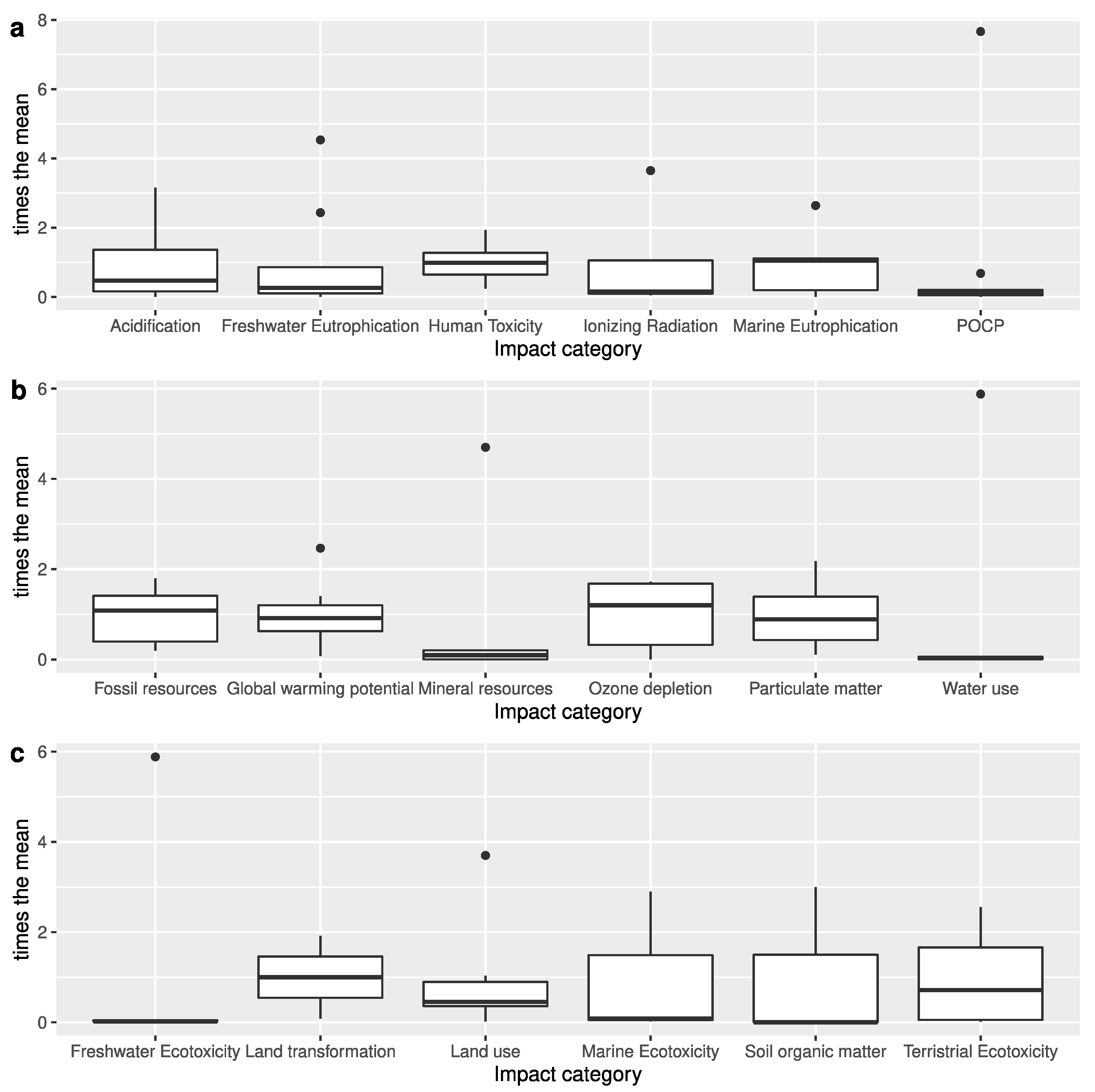
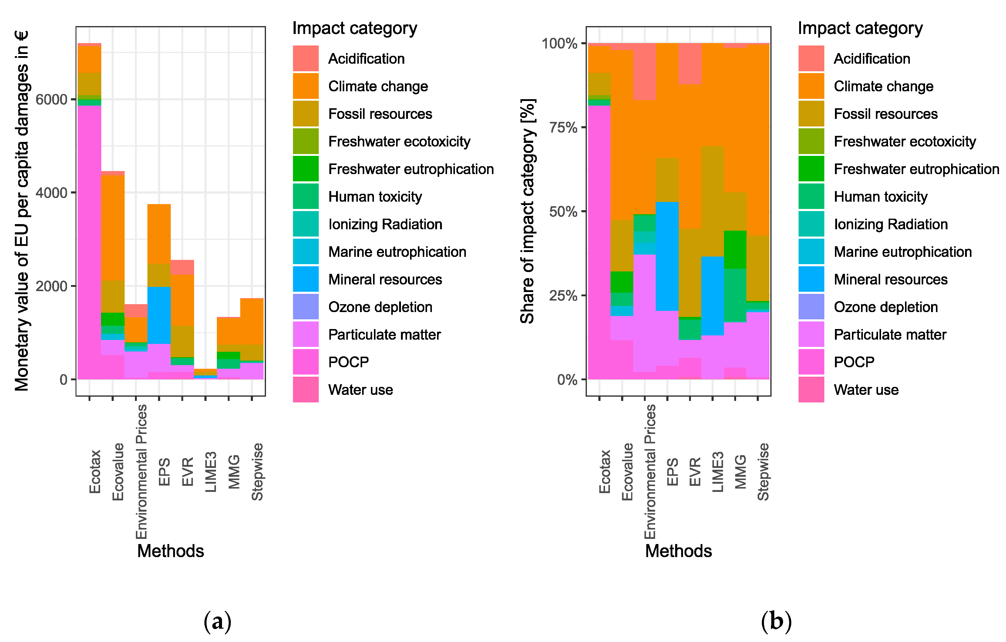
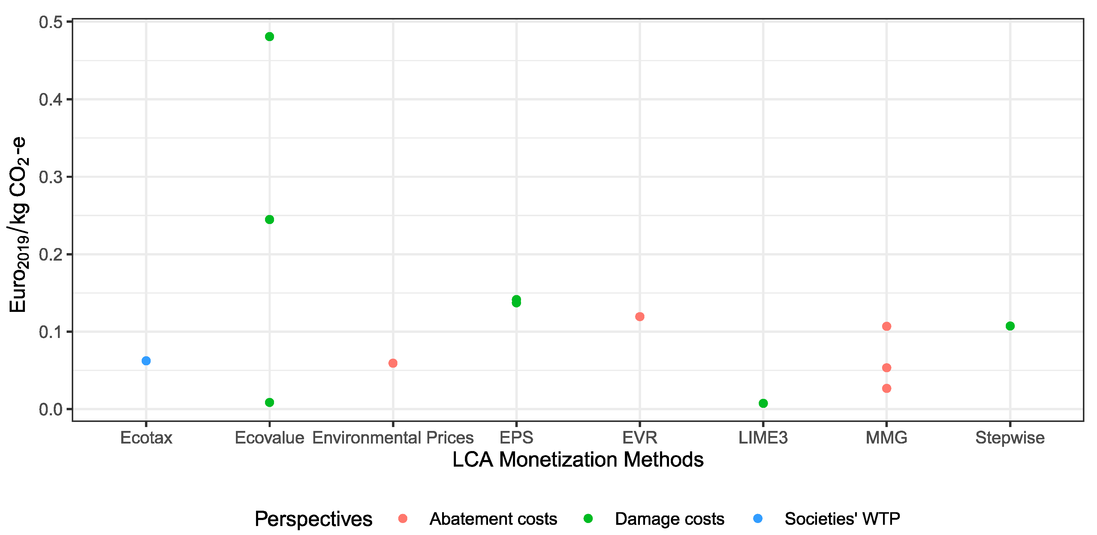
3.2. Quantitative Assessment and Comparison of Different Methods

In Table S3 in the supplementary material, the different monetary values of the analyzed methods for the 18 impact categories that have been determined by the quantitative comparison are displayed. They can also be used as guidance in determining which impact category is covered by which method. In Figure 3, we show the quartile distribution of the different impact categories.

To be able to show the distribution of all values in one graph, we have divided all values by their mean. The values for human toxicity are nearly forming a normal distribution around its median, while eutrophication shows some outliers with a lot higher values and a fat tailed distribution to the right. Impact categories, where the underlying impact assessment is similar, such as photochemical oxidation, global warming, ozone depletion or methods with similar underlying data such as human toxicity or particulate matter, have a more even distribution, while nearly all impact categories linked to ecosystems show very high spreads in their values (freshwater ecotoxicity & terrestrial ecotoxicity, freshwater eutrophication, acidification). The impact categories that have a closer link to human health such as human toxicity and particulate matter show a normal distribution. To determine whether the methods with the damage costs perspectives converge, a brief analysis showed that these distributions only become slightly narrower if we exclude EVR and Ecotax and are still not-normally distributed (see Figure S1 in the Supplementary Material).

Now the results of the overall ranking are discussed. They show which method delivered the highest and lowest result across all impact categories (as described in Equation (7)). The ranks are not to be interpreted normatively; they just underline which methods delivered comparatively the highest and lowest monetary factors per environmental impact. The results are shown in

Table 3. Methods and associated ranks.

Method	Rank
Ecovalue	1
Ecotax	2
Environmental Prices	3
EVR	4
MMG	5
Trucost	6
EPS	7
Stepwise	8
LIME3	9

.

Based on the ranking of the inter impact category comparison, the Ecovalue method had the highest values, followed by the Ecotax method, the Environmental Prices, EVR, the MMG method, and finally Trucost, EPS, Stepwise and LIME3. This means that the Ecovalue method had on average the highest values across all impact categories and LIME3 the lowest. The interpretation of the magnitude of the values are compared on a per impact category basis in Section 3.3. However, when we consider the broader picture, it seems that the geographical scope of the methods plays an important role: both approaches that cover Sweden (Ecovalue and Ecotax) have the highest value, while the three following methods (Environmental Price, EVR and MMG) have European coverage. The methods with the lowest values (Trucost, EPS, LIME3 and Stepwise) have a global scope. Interestingly, a slightly higher value for human health as provided by Stepwise does not play a significant role in increasing the results, apart from those impact categories that are strictly connected to human health such as particulate matter. Another interesting finding is that the methods that assess abatement costs do not show strictly higher or lower values than the other methods.

In the final step of the quantitative assessment, we multiplied the obtained monetary values of the emissions with the emissions and resource demands of an average EU citizen. The results are displayed in Figure 4.

It is visible that the monetary damages associated with per capita emissions show a wide range. The Ecotax method obtains a value of nearly 8000 € of damages associated with average EU per capita domestic emissions and resource demands in 2010. The total per capita damages yielded by the LIME3 method were 224 €. In line with the observation in Ecotax and Ecovalue yielded the highest results. Discounting may also play a role as the obtained monetary value of Environmental Prices and MMG, that use a 3% discount rate, are the 6th and the 7th lowest, respectively. EPS and Stepwise have a higher value for the damages per capita, as impact categories in which they provide higher values (e.g., climate change and fossil resources) constitute a large share of the overall damages.

However, not only the associated damages of the total damages per capita vary: also, the shares and the weighting in between the impact categories differ, as can be seen on the right side of Figure 4. For the Ecotax method over 80% of its damages occur due to POCP emissions. Climate change is rated consistently quite high over all methods (with 7% as the minimum for the Ecotax method). Freshwater eutrophication, marine eutrophication, ionizing radiation, water use and acidification are rated quite low (under 10% with an exception for the MMG method for freshwater eutrophication (11%) and acidification (17% for Environmental prices and 12% for EVR)). In addition, the valuation for human toxicity and particulate matter varies between 1% (Stepwise) to 16% (MMG) and 5% (EVR) to 35% (Environmental Prices), respectively. For some values, the obtained weighting is very alike though: for ozone depletion all methods provide a weight of under 1% and for freshwater ecotoxicity under 2%.

Impact categories that have a strong link to biodiversity such as eutrophication, acidification and ecotoxicity have only very low shares of the monetized damages. However, other impact categories with a strong link to biodiversity such as land use and marine and terrestrial ecotoxicity had to be excluded because of limited data availability or compatibility with the impact category indicators. An inclusion could change this observation.

3.3. Integrated Qualitative Comparison and Quantitative Assessment

In the following, the results for the individual mid-point impact categories for which more than two methods provide a quantitative assessment are presented. The qualitative and quantitative results per impact category are discussed together. The values for the method Trucost had to be excluded as the associated values are not published.

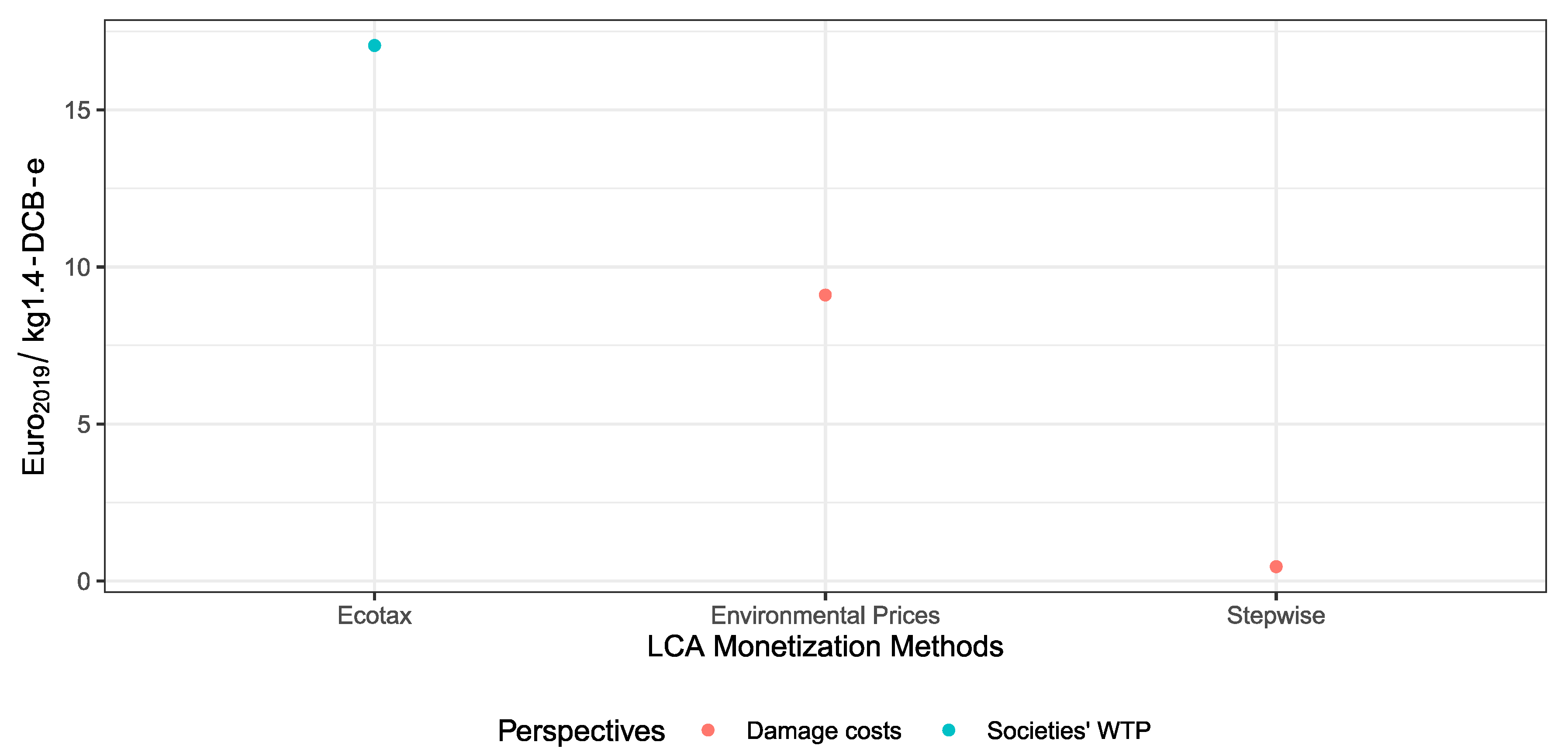
3.3.1. Climate Change

Eight methods provide monetary values for climate change. The lowest value is given by LIME3 (under 0.75 ct per kg or about 7.5 euro per ton). The highest value is provided by Ecovalue maximum estimate which is 50 ct per kg of CO₂-e, resulting in an emission damage of 500 € per ton. The values are displayed graphically in Figure 5. Some methods (Ecovalue and MMG) provide min and max values so that several values per method are visualized.

The values spread over two orders of magnitude, which is in line with the results by Dong et al. [21].

Ecovalue08 used the values by the Stern Review and the FUND model [33,88]. It is not clear which value Finnveden and Noring [62] use in the Ecovalue12 update as they state several references ([89,90,91,92]) but not a clear calculation method. As these are all publications on integrated assessment models (partially the FUND model and the DICE model), we assume therefore that it contains damages to agriculture, human health and ecosystems. Overall, the four methods Ecovalue, EPS, LIME3 and Stepwise use damage cost and integrate damages to/on human health and biodiversity.

The lowest values are derived from LIME3 and the low estimate of the Ecovalue method (under 10 €/ton). The fact that the value for LIME3 is so low is not surprising as it has relatively low AoP valuation for human health (see Table 2). EPS covers mainly damages that are otherwise associated to integrated assessment models such as increased heat stress. The reduction of working capacity consists more than half its value (as stated by Dong et al. [21]) and is responsible for its very high value.

For the three methods using the abatement cost approach (MMG, Environmental Prices and EVR), the results do not differ significantly. The MMG method mainly uses abatement costs but also other cost calculation approaches. Environmental Prices uses abatement costs. EVR uses abatement costs to reach the Paris Agreement, e.g., needed investment in offshore wind parks; this is maybe why its abatement costs are slightly higher than the other methods.

One aspect that should be noted is that the MMG method uses different CO₂-prices for its buildings depending on when they are emitted in the building’s life cycle. This is not in line with the ISO 14067 [93], which does not allow to account emissions with different emission times to be accounted for differently. This is challenging to combine with monetized CO₂-prices in integrated assessment models, as these are usually time differentiated and use a discount rate.

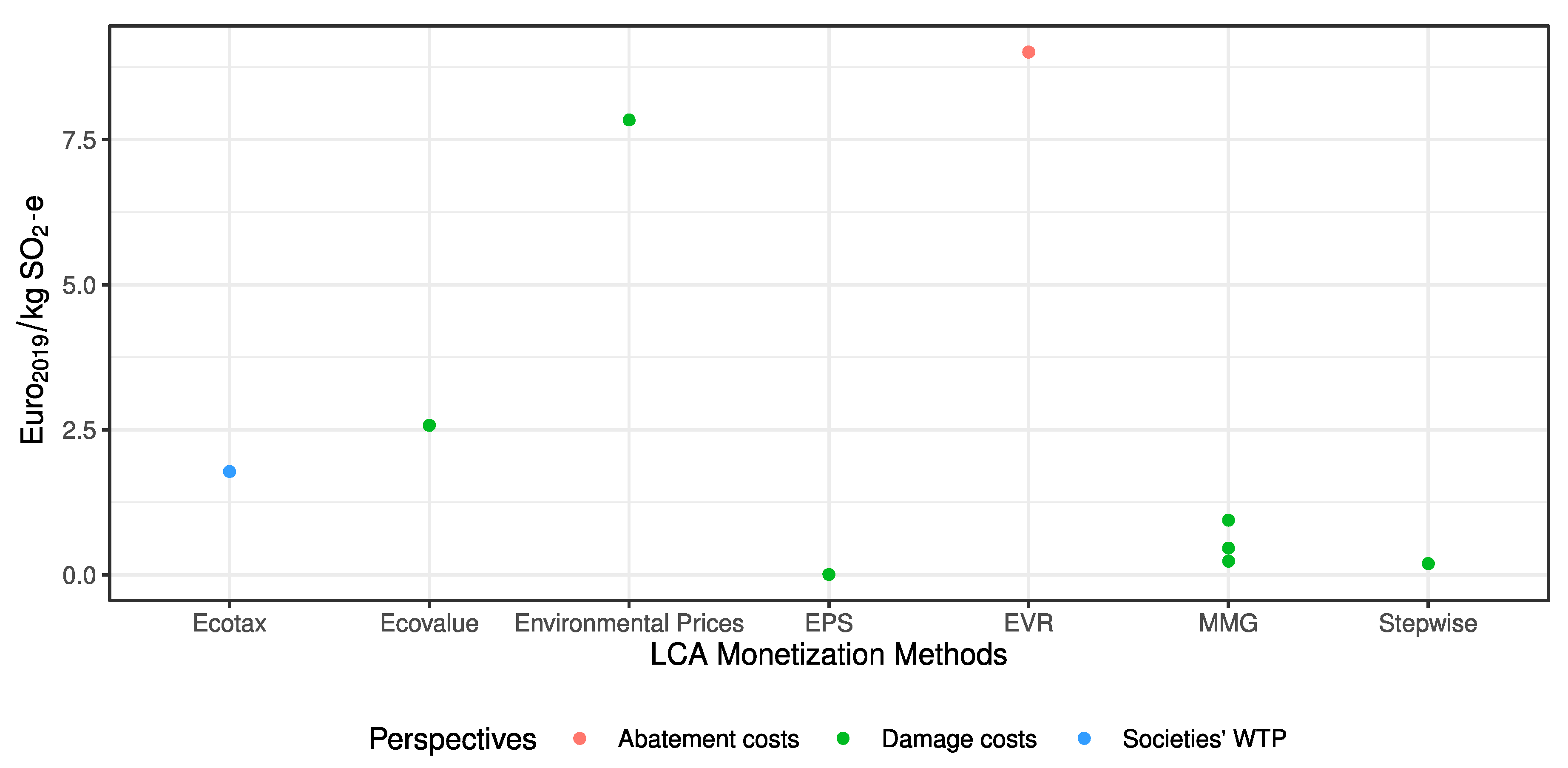
3.3.2. Acidification

Seven of the assessed methods published damage values for acidification and their quantitative comparison are displayed in Figure 6.

With values between 0.01 € per kg SO₂-e (EPS) and 9 €/kg SO₂-e (EVR) we have again a spread of two orders of magnitude. For EVR, the costs are the costs associated to ultra-low Sulphur content diesel, which cannot be compared to the damage costs. It is noteworthy that in the impact category acidification the abatement costs seem to be higher than the damage costs. The Ecotax method considers taxes on Sulphur content in fuels, which would be too weak a financial incentive to implement the technology suggested by the EVR as it costs more than three times the tax.

Four methods in the impact category acidification use the damage cost approach. Three of these have values under 1 € /kg SO₂-e (EPS, MMG and Stepwise), while the Environmental prices seems to be an outlier with a higher value.

EPS includes all damage endpoints for acidification (species, corrosion and ecosystems), but still has the lowest value. The Stepwise method only includes damages to ecosystems. This explains why its impact is so low [65]. For the EPS, the low values can be partially explained by average, not marginal, damages. The Ecovalue monetary value is higher than the value for Stepwise, MMG and EPS. This is not surprising: their geographical scope is Sweden, so that it is likely that the damages are valued higher due to the higher income of Swedish citizens. Since the values are derived by contingent valuation, they also include wellbeing.

The Environmental Prices value is presumably that high because it provides a higher estimate of biodiversity and ecosystem services (because its values are based on Kuik et al. [82], and not on Ott et al. [80]). Further, the LCA weighting factor is equal to the medium estimate in the handbook that also includes building damages which are based on the NEEDS project [83]. The building damages for Environmental Prices exceed the entire damages of Stepwise and EPS (0.6 € per kg SO₂ only for buildings [29]). It should be noted that the values provided for SO₂ and its associated damages vary by an order of magnitude in the Environmental Prices Handbook (compare Tables 1, 3, and 33 in the Environmental Prices Handbook [29]).

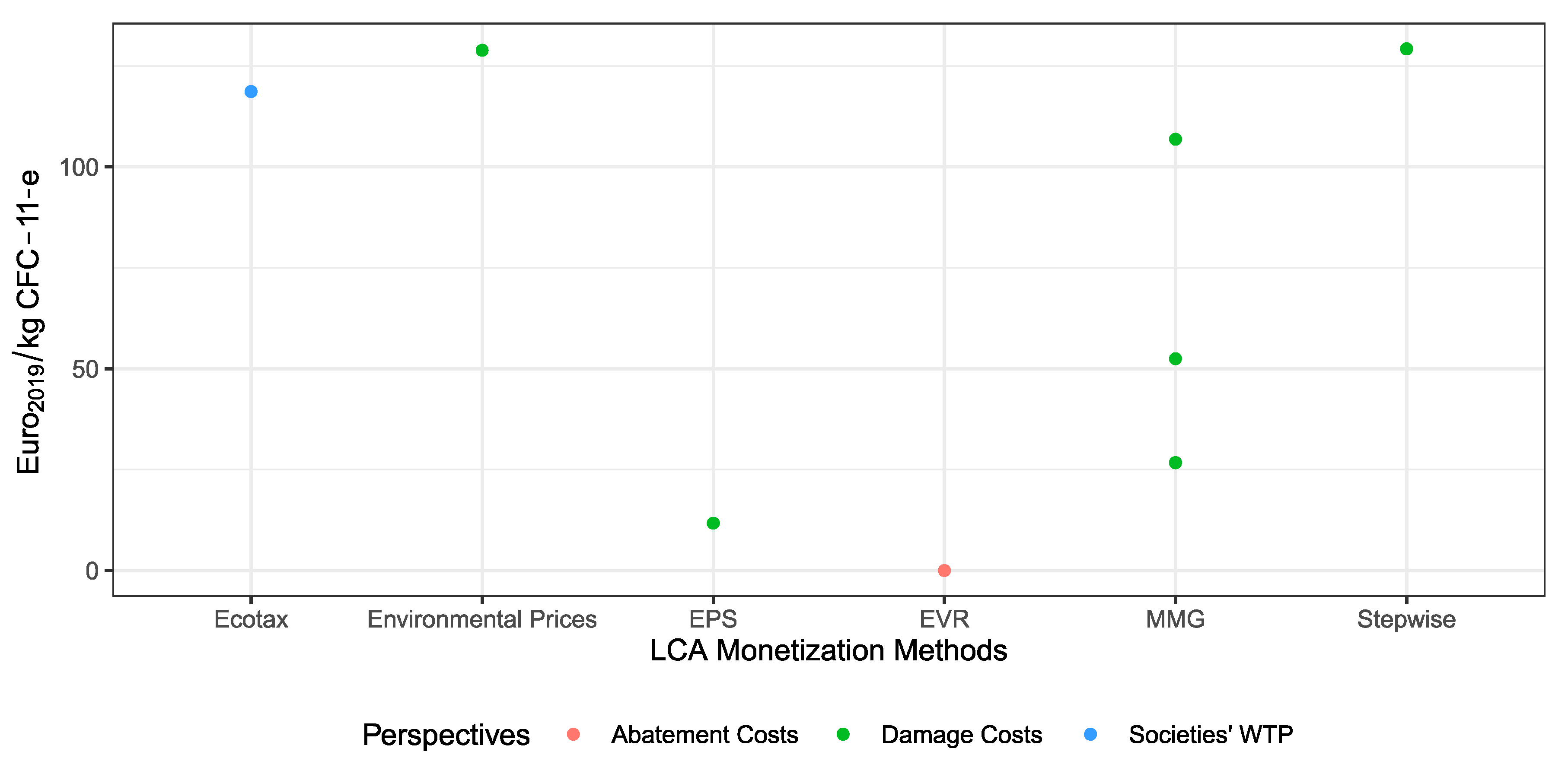
3.3.3. Ozone Depletion

Six methods assess the monetary damages of ozone depletion. For ozone depletion, the results have a spread of one order of magnitude if we exclude the zero value. EVR has the value of zero, while three of the other methods have a value of just over 100 € per kg of CFC-11 (see Figure 7). We can see in the plot that the values are very similar, apart from the MMG method low and central estimate, EPS and the EVR method. That is because the damages are quite high, while the abatement costs are very low. The lowest values are yielded for the abatement costs, since the EVR method concludes that it does not cost anything to prevent CFC-11 emissions. For the damage costs, Stepwise and Environmental Prices have the highest values.

For the value obtained by Environmental Prices, damages to human health and ecosystems are included. For the EPS, the impact of the pure ozone depletion value is 11.21 €/kg. EPS only assesses health damages here (skin cancer and sight problems), and no damages to ecosystems. Stepwise includes human health impacts and impact on working capacity [65]. The MMG method considers health damages, damages related to agricultural damages and material damages based on the old shadow prices Handbook (2010) and the ReCiPe version of 2008 [94]. Stepwise had slightly higher associated human health values and includes working capacity. This can explain the higher values of Stepwise. However, the EPS has a high associated value for human health, but yields the lowest value for stratospheric ozone depletion, which is inconsistent. One reason for this inconsistency could be due to marginal and non-marginal impacts; because the EPS provides non-marginal values and all other methods use marginal analysis. In addition, the EPS does not include ecosystem nor working capacity damages. Another aspect that influences the magnitude of the results is the time perspective. As the time perspective of ozone depletion is long, the values are sensitive to the underlying reference scenarios.

3.3.4. POCP

Eight methods assess the environmental impacts of POCP (see Figure 8).

The range of the POCP values is high. We have an outlier (which can also be seen in the respective boxplot in Figure 3) with the value provided by the maximum value of Ecotax (763 €/kg), potentially attributable to its method and its geographical scope. The lowest values are provided by the low estimate of the MMG method, which provides a value of 0 €. The basis of the Ecovalue data, which has the highest value after the Ecotax method, is difficult to trace back: Finnveden and Noring [62] deliver no new sources, while the source given by Ahlroth and Finnveden [59] (that published the previous Ecovalue model), the Methodex Project website, is no longer accessible nor existent on the internet [95]. However, Ahlroth and Finnveden [59] state that the Methodex project includes POCP damages on human health (valued through contingent valuation) and agricultural yield losses that are measured through market price. The third highest value is provided by the EPS which includes crop loss, wood loss, asthma and increased COPD cases, but its value is just over 1 €/kg of C₂H₄-eq. The Environmental Prices approach only includes chronic health impacts of POCP and is even lower than the values delivered by the EPS. Stepwise has the second lowest values even though it includes damages to four endpoints and has a very high underlying value of human health. EVR also provides low values since avoiding POCP emissions seems relatively cheap. The MMG method has higher values than Stepwise and Environmental Prices, but lower values than EVR and EPS. It bases its valuation on the ExternE project and on the program EcoSense, therefore accounting for public health mainly, but also for crop damages [96]. Details of how values are corrected for inflation etc. are not provided. LIME3 has the lowest obtained value. It only includes damages to human health, and the respective valuation of the AoP human health is relatively low compared to the valuation of the other studies. Overall, the results are not completely explainable related to AoP valuation. Different impact assessment models, the applied unit conversion factors (as the different monetary values were provided as NOx-e, NOVOC-e, C₂H₂-e and had to be converted with unit conversion factors documented in Table S1 in the supplementary material) and the mechanism of POCP creation that is geographically very varied can be elements explaining the observed differences.

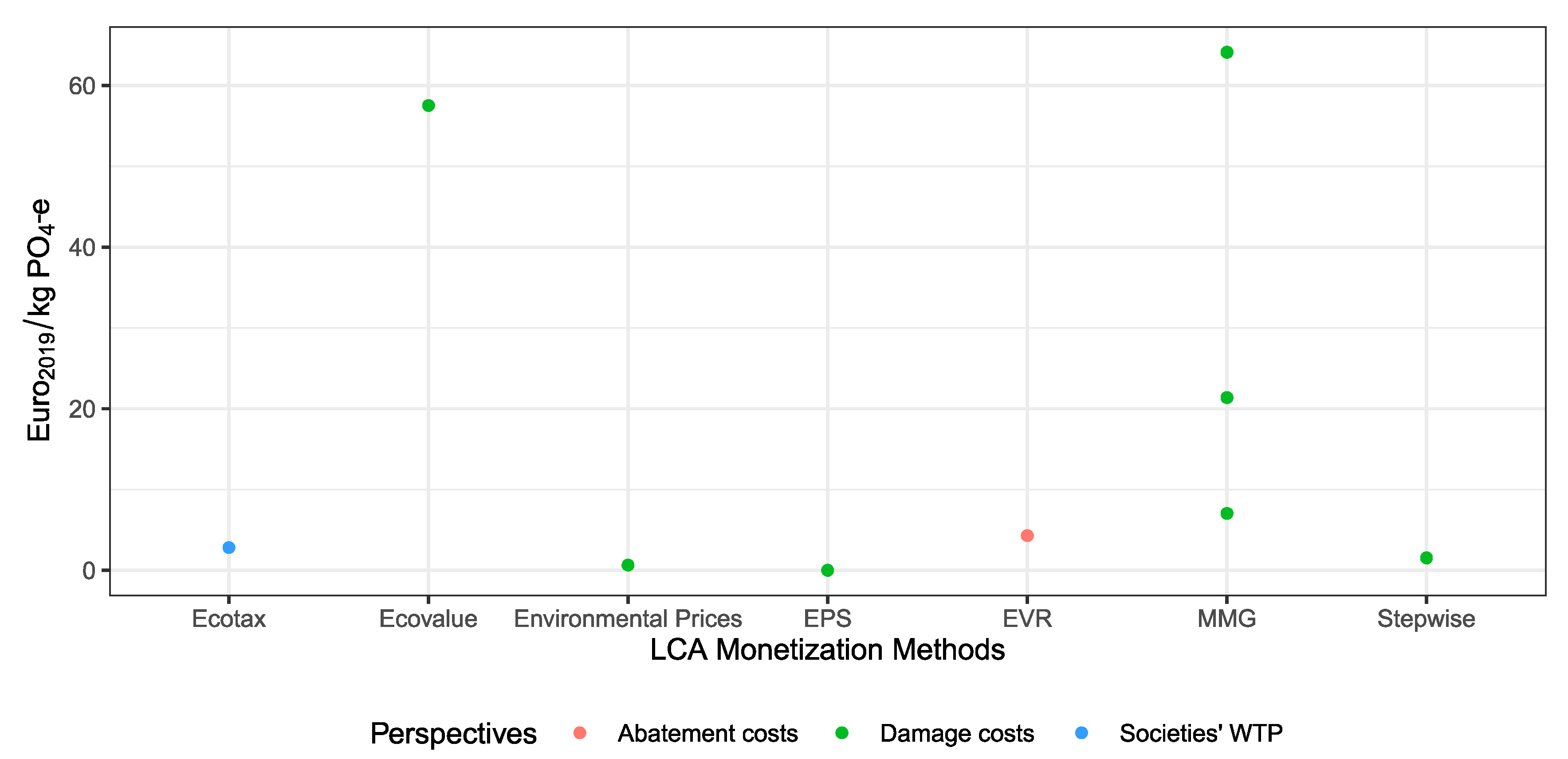
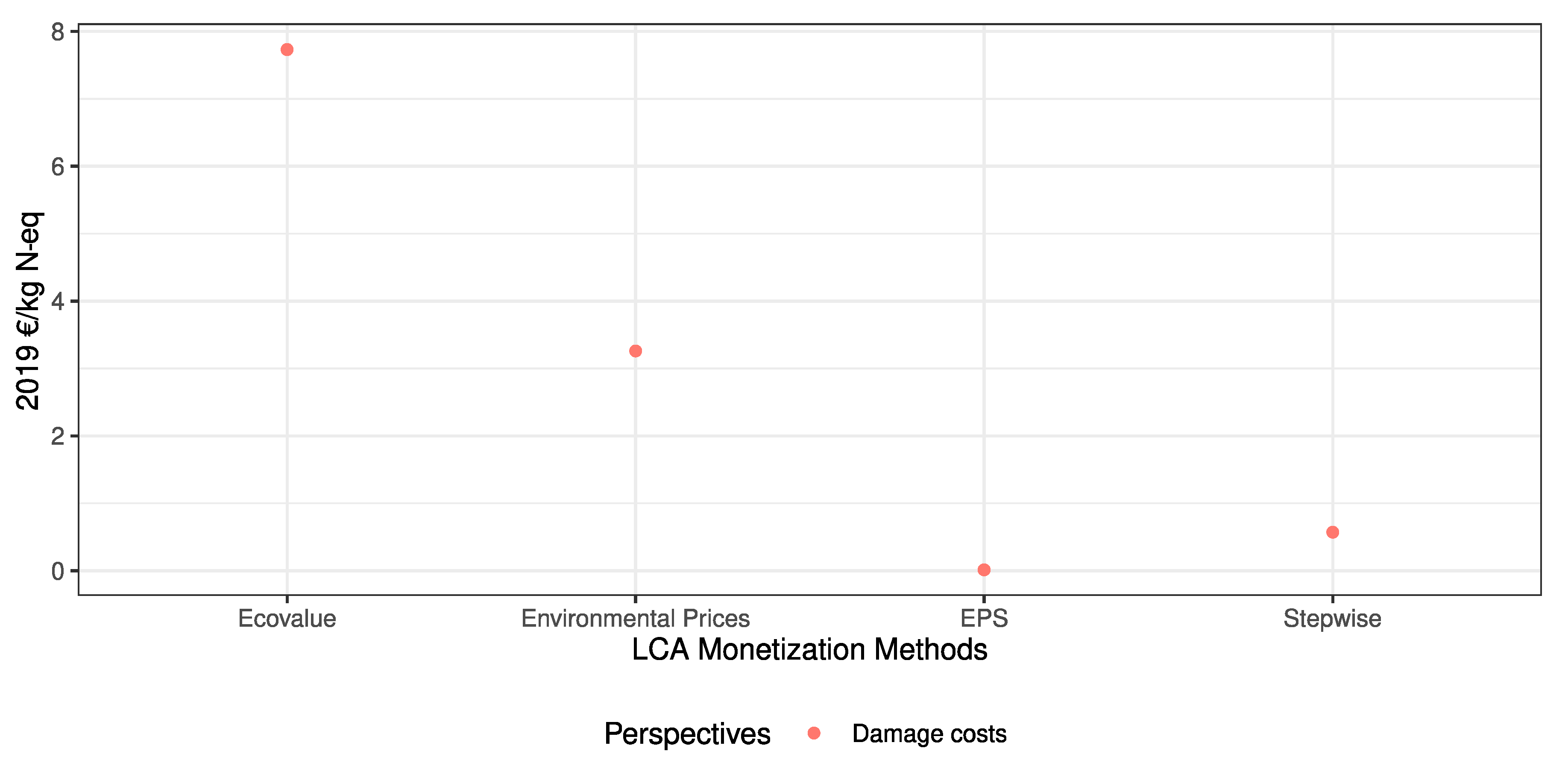
3.3.5. Eutrophication

The impact category eutrophication is covered by seven of the analyzed methods, while three methods (Ecovalue, Environmental Prices, EPS) also address marine eutrophication explicitly, while others do not distinguish between the two and only assess aquatic eutrophication (like Stepwise). Since the distinction is not always available, differences in the results can also occur due to different scopes of the impact categories. The results range from 64 €/kg PO₄-e (upper bound MMG-method) to just over 1 ct (EPS) (as visible in Figure 9).

The MMG method’s highest value is the highest estimate. One reason for the high value of the Ecovalue method can be its development context: Swedish peoples’ WTP was estimated to reduce eutrophication. The values from Finnveden and Noring [62] were not updated and are based on contingent valuation studies and travel cost methods from Ahlroth [60]. Since the GDP per capita in Sweden is higher than in other countries, it is also logical that the WTP is higher, since the WTP is wealth sensitive. Already Ahlroth et al. [59] noted that the Ecovalue values are a lot higher than the Ecotax values (that are based on taxes on nitrogen in fertilizers). They concluded that the current environmental tax on eutrophic substances is too low and actually lower than what people in Sweden would be willing to pay. The Ecovalue study also includes the recreational value a lake delivers if it is not eutrophic (and therefore includes wellbeing beyond health). The inclusion of agricultural and ecosystem damages is not explicit, because the assessment in the Ecovalue method does not ask for the reduced biotic production nor for a link from emission to species but for WTP for an increased sight depth. However, stating that species richness is included in this assessment would imply letting the survey participants guess the cause-effect chain between sight depth and species richness.

The MMG method provided values for Eutrophication (damage costs and prevention costs) [75]. The overall range of the results is very high, especially the damage costs that are based on a willingness to pay study to reduce eutrophication in the Baltic sea [97]. Therefore, the values relate to marine eutrophication rather than to freshwater eutrophication. Interestingly, both methods (MMG and Ecovalue) that include contingent valuation deliver the highest values.

The lowest values are yielded by the EPS, which analyses the average impact based on global phosphorous flows [98] and their impacts on species richness. Additionally, the impact on agricultural productivity is covered. Environmental Prices provided the second lowest value. Its assessment only includes effects on biodiversity (PDF) based on ReCiPe.

Stepwise obtained a higher value than Environmental Prices; it also includes only damages to ecosystems and is based on the impact assessment of EDIP 2003. Stepwise values are presumably higher than Environmental Prices because its underlying valuation of biodiversity is also higher (see Table 2).

Only three methods assess the impact category marine eutrophication explicitly. The Environmental Prices method assesses the values based on ReCiPe 2013 and its according PDF with the method by Kuik et al. [82] (transferred its approach to water). The monetary values in €/kg of N-e are displayed in Figure 10.

Ecovalue assesses the value based on a contingent valuation study and travel cost method based on the same approach as above. Again, the high GDP in Sweden might explain the high values for the Ecovalue method. Stepwise includes, as mentioned above, only the damages to ecosystems and has a quite low estimation of the associated values (as no distinct value for marine eutrophication is provided, only a value for generic aquatic eutrophication). However, Environmental Prices included only damages to ecosystems, but yielded a higher value than Stepwise, which is in conflict with its lower biodiversity valuation compared to Stepwise. The EPS provides a value for marine eutrophication impacts and considers damages to agricultural production as well as ecosystems, and provides the lowest value as for freshwater eutrophication.

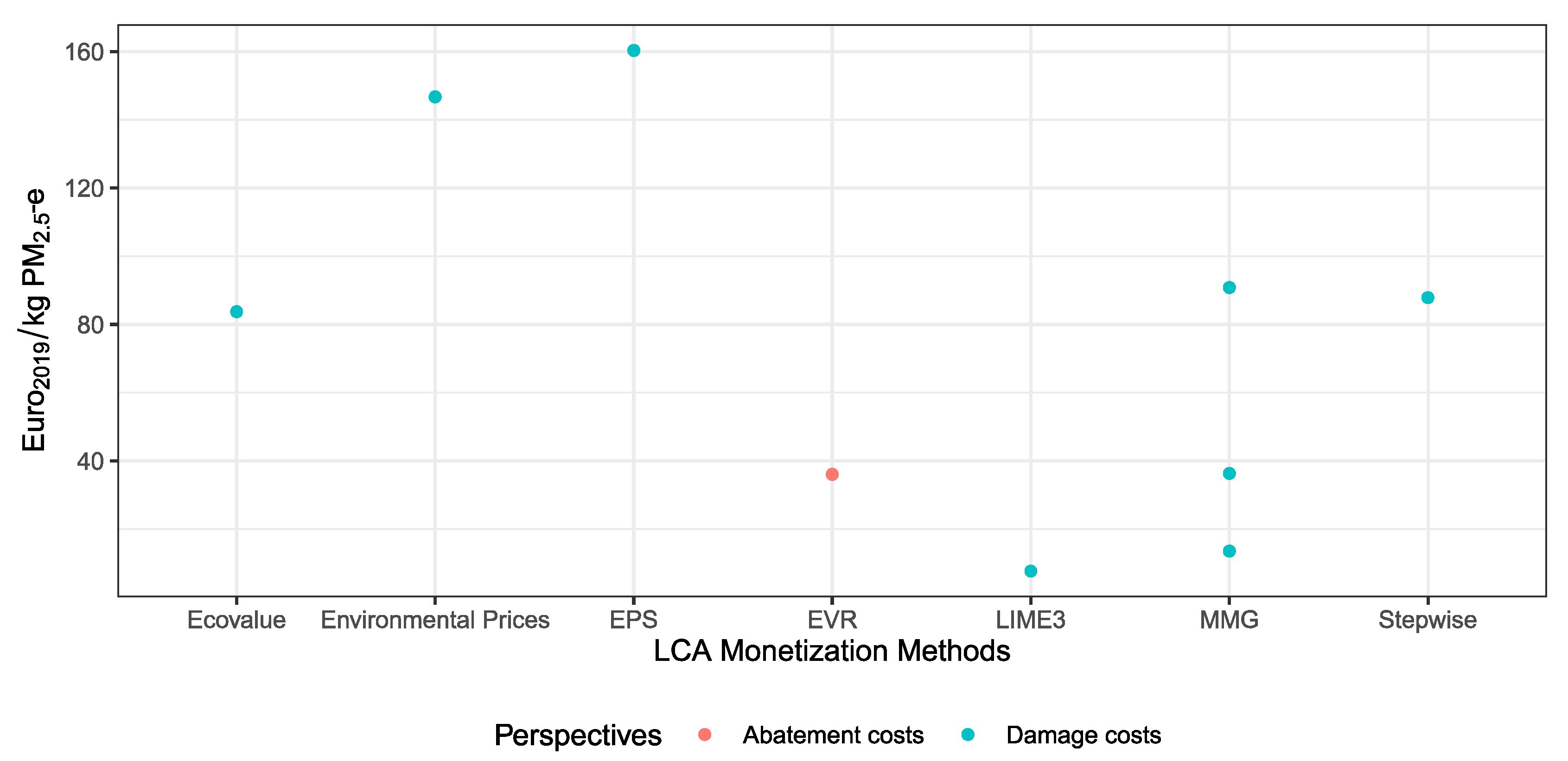
3.3.6. Particulate Matter

Seven methods cover the impact category particulate matter. The highest value is provided by EPS (160 € per kg PM_2.5-e) and the lowest value by LIME3, which is just over 7.7 € per kg PM_2.5-e. Therefore, the results spread again over two orders of magnitude. As particulate matter has mostly impacts on human health, and all methods that use damage cost have similar valuation of human health, it is surprising that the values are so different. The values are displayed in Figure 11.

It cannot be precluded that the conversion factor is responsible for the magnitude of the Environmental Prices value: we used TRACI conversion factors [54] (as documented in Table S1) because ReCiPe did not provide a characterization of PM₁₀-e (which is the impact assessment indicator of Environmental prices, but all impact assessment methods should have the unit PM_2.5-e). The CFs used by TRACI suggest that the impacts of PM_2.5 are about four times as harming as PM_10. While the method by van Zelm [99] supports this order of magnitude, Gronlund et al. [100] suggest that the impact of PM_2.5-e is less than twice as harming as PM₁₀-e. In addition, the value for EPS is very high, which is in line with its value for human health. The same is true for the Stepwise values, which are lower despite including reduced working capacity. The EVR value is low, suggesting that it is cheaper to abate particulate emissions than to endure their associated damages. Ecovalue’s slightly higher value might be due to the Swedish geographical reference area, with a relatively higher GDP. In addition, here the values are converted from PM₁₀-e. The background data of the Ecovalue method are those used by the Shadow Prices Handbook [101] before the Environmental Prices update. It only includes damages to human health. If PM₁₀ was assumed to be as harmful as PM_2.5, then Stepwise would have the second highest value, because the values by Environmental Prices and Ecovalue would be lower than the Stepwise value. Environmental prices also included material damages of particulate matter. The differences between the methods cannot be deduced only by the different valuation of human health. Rather it is reasonable to assume that they are caused by different impact assessment and geographical reference, as particulate emission’s damages highly depend on the exposed individuals and therefore on transport models and population density.

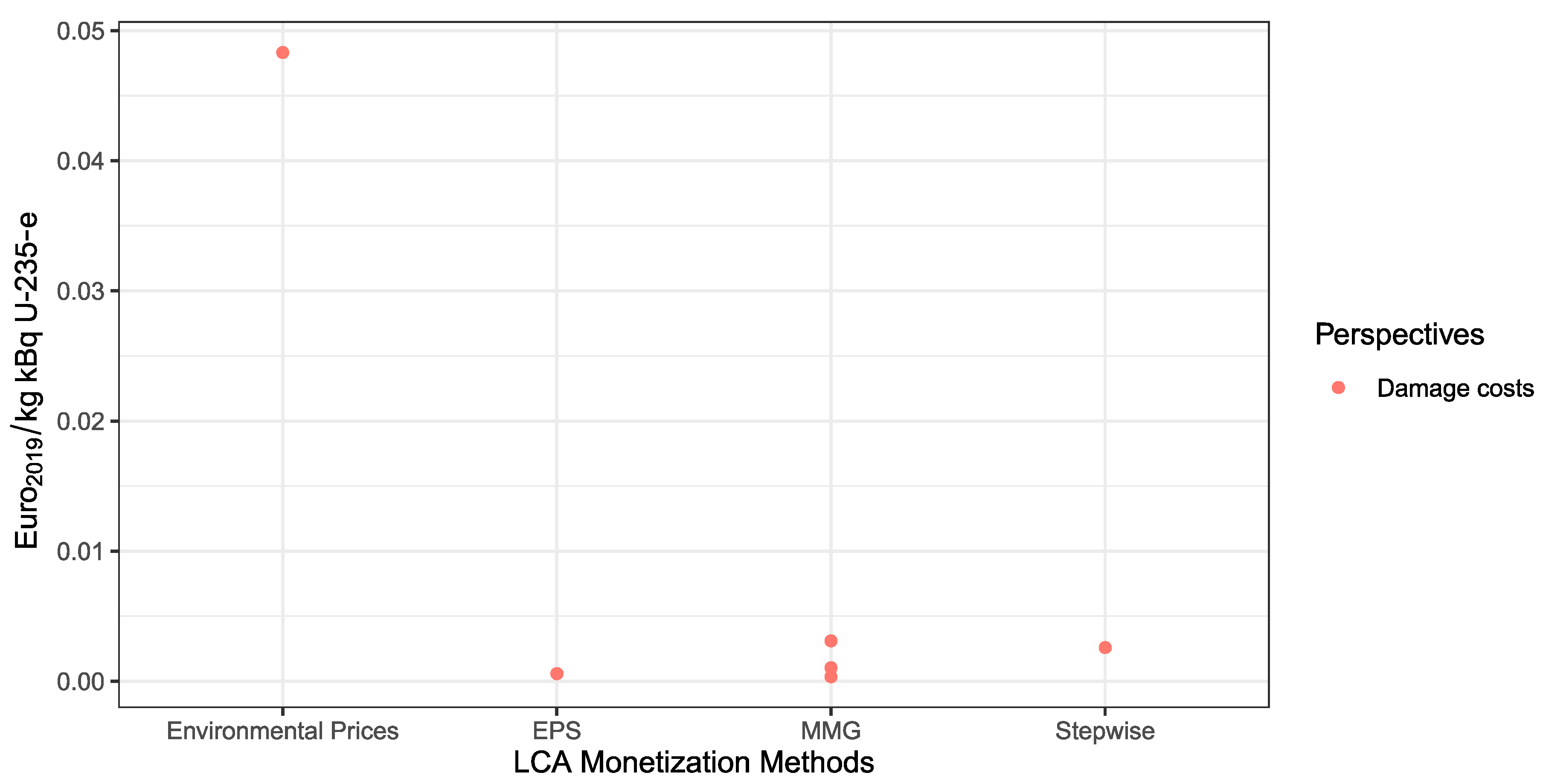
3.3.7. Ionizing Radiation

Four methods cover the impact category ionizing radiation: Environmental Prices, Stepwise, EPS and the MMG method (displayed in Figure 12).

The provided results per kg kBq U235-eq are very different. The max-value MMG method is 20 times lower than the value for Environmental Prices. This difference is not really explainable as both methods are based on ReCiPe; The MMG assessment is based on ReCiPe 2008 [94] and Environmental Prices on the 2013 ReCiPe update [102]. All assessed methods use the damage cost approach and consider human health damages only. Stepwise uses the Impact 2002+ impact assessment method and EPS uses data based on cancer incidences based on its former version. As all methods have a similar magnitude in their human health valuation, the high spread of the results is not explainable by our qualitative criteria. Owsianiak et al. [48] found large differences in the impact assessment of ReCiPe and Impact 2002+ for the impact category ionizing radiation. While this can explain the difference between the Stepwise and Environmental Prices methods, it does not help understanding the difference between the Environmental Prices and MMG methods.

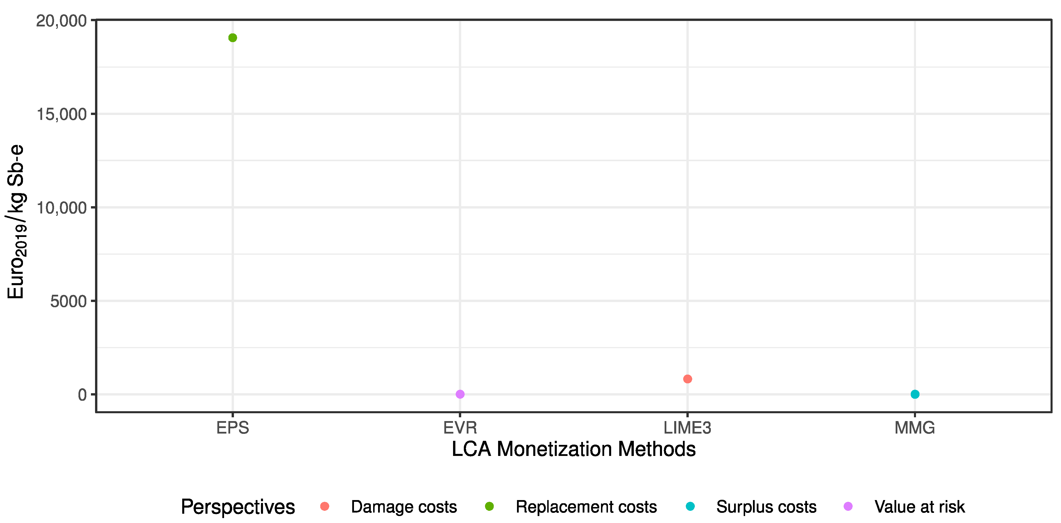
3.3.8. Mineral Resources

Four method delivered monetary values for mineral resources, but they are very challenging to compare as many different approaches were taken. The external costs per unit of Sb-e (antimony equivalents) range from just under 20,000 €/kg to 0 € from the MMG low estimate which assumes that all external costs are already included in the market price (see Figure 13).

Environmental Prices discusses the challenge of resource scarcity but does not provide quantitative weighting factors for LCA. It states that its approach is based on the Hotelling rule [103]. Overall, the method’s approach to monetize scarcity does not fit well in the scope of our cost perspective classification from Section 3.1, apart from LIME3 that has been obtained by stated preference studies and therefore is classified as determining damage costs.

Even though the EPS value seems to be an outlier compared to the other methods, the LIME method also provides a value of over 800 €/kg of Sb-e, while the value for EVR and the MMG high estimate are around 10 €/kg Sb-e. Therefore, the results are spread across five orders of magnitude (excluding the zero value for MMG low) and have so far the widest range.

EPS takes the replacement cost approach (so how expensive will it be to obtain a material if no further ore of it is provided), while EVR works with a quantification of value at risk/supply risk. The MMG method with the lowest value used the ReCiPe approach that is also based on surplus costs.

The high associated values for EPS are underlined by the fact that for the EPS scheme the AoP resources seems to be the most important one [28]. The EPS method assigns a high value to the external costs of ores and minerals. These values dominate all versions of EPS.

LIME3 calculates external costs of mineral resources through land use change associated with mining, which is again a different approach compared to the other presented methods.

The MMG values (0–6.65 €/kg Sb-e) are similar to those from EVR (8.1 €/kg Sb-e). As all the methods have very different approaches, it is not surprising that their monetary values also differ.

3.3.9. Fossil Resources

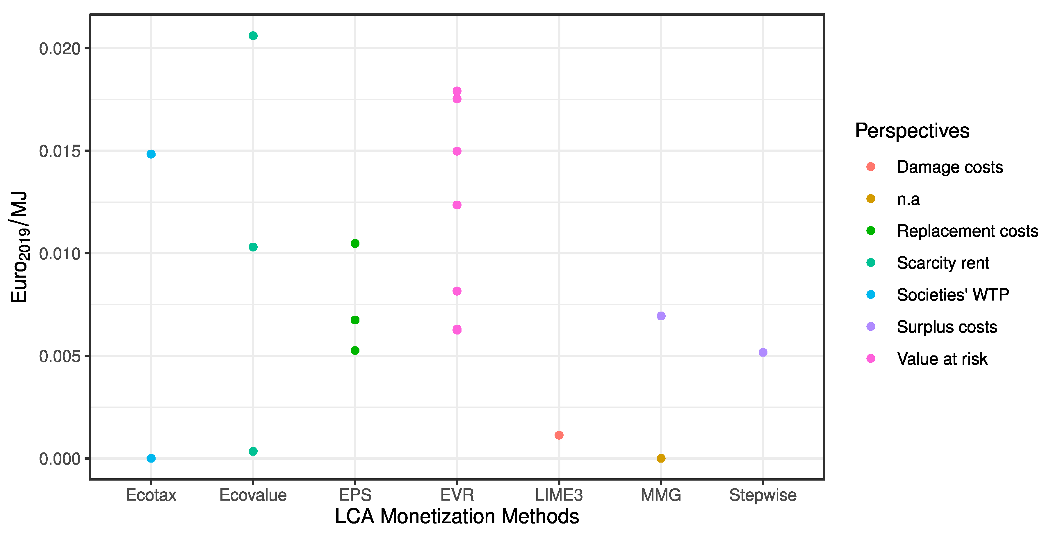
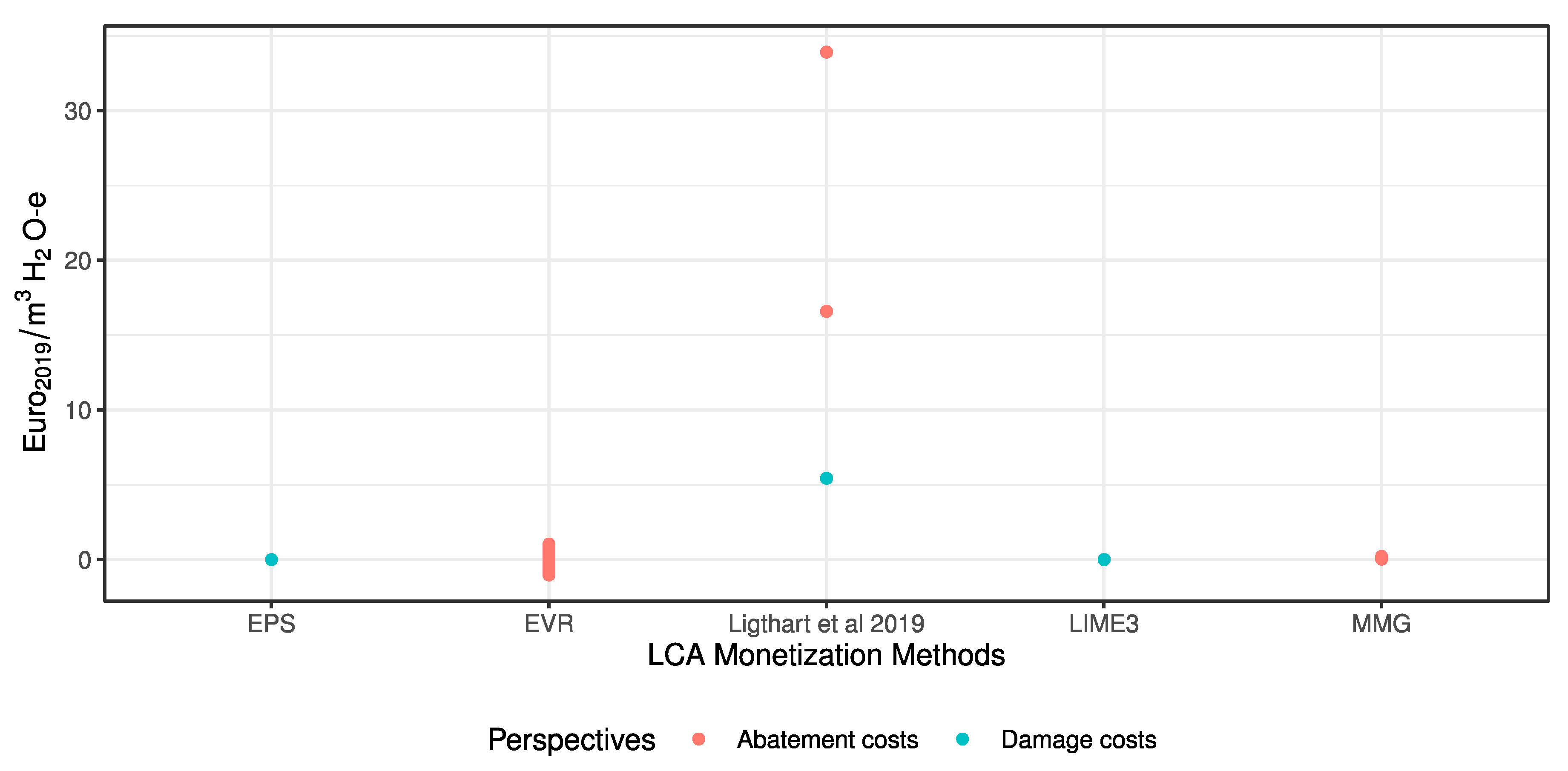
For fossil resources, seven methods provide monetary factors. The values were scaled to the unit €/MJ. All methods obtain a value of under 3 ct per Mega joule (see Figure 14).

As for the cost perspectives for mineral resources, the taken approaches are difficult to classify with the classification that we have used so far. While the Ecotax method is based on taxes for mineral resource use, which is low, the Ecovalue approach is based on resource rent data.

For the Stepwise method, it is difficult to determine where the values come from. The value used here is from Pizzol et al. [20], while it seems that in Weidema et al. [65] the external cost of European fossil fuels with Stepwise is zero. Therefore, the approach is unclear. It is based on the approach by IMPACT 2002+ [52], that is based on the Eco-indicators surplus cost approach, which is close to the approach used in ReCiPe.

The MMG method assumes, for the central and low value, that resource values are internalized in prices and therefore applies a value of zero. The high value includes the approach in the Ecoindicator 99, which is the surplus costs approach, and military costs to secure resources. However, EPS assesses how costly it would be to produce the same amount of energy from renewable resources (converting wood to oil by Fisher-Tropsch-process or charcoal and biogas production), while EVR has a method to determine value of risk. Both assessments are not provided by values per MJ, but by value per mass of different energy carriers. This is why both methods deliver a variety of values that were obtained by a conversion through caloric values of different fuels (see Table S1 for more information). LIME3 uses the same approach for mineral and fossil resources: it calculates the overexploited economic values by current resource production as an economic externality of mineral and fossil resources use based on the El Serafy’s use cost approach.

Because of those very different approaches, (none is used twice apart from the MMG high estimate and Stepwise), it is surprising how narrow the distribution of the values is (even though the results range again between two orders of magnitude if the zeros are left out).

3.3.10. Water

Five different methods include the impact water use. The costs range from costs under one cent per cubic meter to over 30 € per cubic meter (see Figure 15) and thus range over three orders of magnitude.

The method by Ligthart and van Harmelen [104] determines marginal abatement costs and marginal damage costs of one cubic meter of H₂O-e based on the impact assessment from Frischknecht et al. [50]. It is included because it is the newest study for shadow costs of water and has an explicit connection to LCA. The abatement costs are determined through the cost of technologies that reduce water use (two different values were provided in the abstract and in the full text- both were considered). The damage costs are based on forgone increased revenues due to irrigation of agricultural products (market price approach). For the EPS the obtained values for irrigation and drinking water are based on costs of drinking water and the assumption that irrigation water costs half the amount of drinking water and therefore they follow the market price approach. The EVR method assessed how to win water back by reverse Osmosis (1 €/m³) multiplied by the baseline water stress according to Gassert et al. [105]. For some regions, it delivers negative values, which we were not able to understand. While the MMG method is based on the Swiss ecoscarcity method as well, the MMG method applied replacement costs, by evaluating technologies that are applied to win water back in countries with a certain amount of water stress. The abatement costs in the Ligthart method are a lot more expensive than the abatement costs proposed by the EVR or the MMG method. The LIME3 value is based on Motoshita et al. [66,106] and includes damages to human health. The values are close to the MMG central estimate that is based on abatement costs. As the damage costs of the Ligthart method and LIME3 cover damages that are completely different in their nature (damages to agricultural goods opposed to damages to human health through malnutrition and infectious diseases), the different values are in line with the expectations.

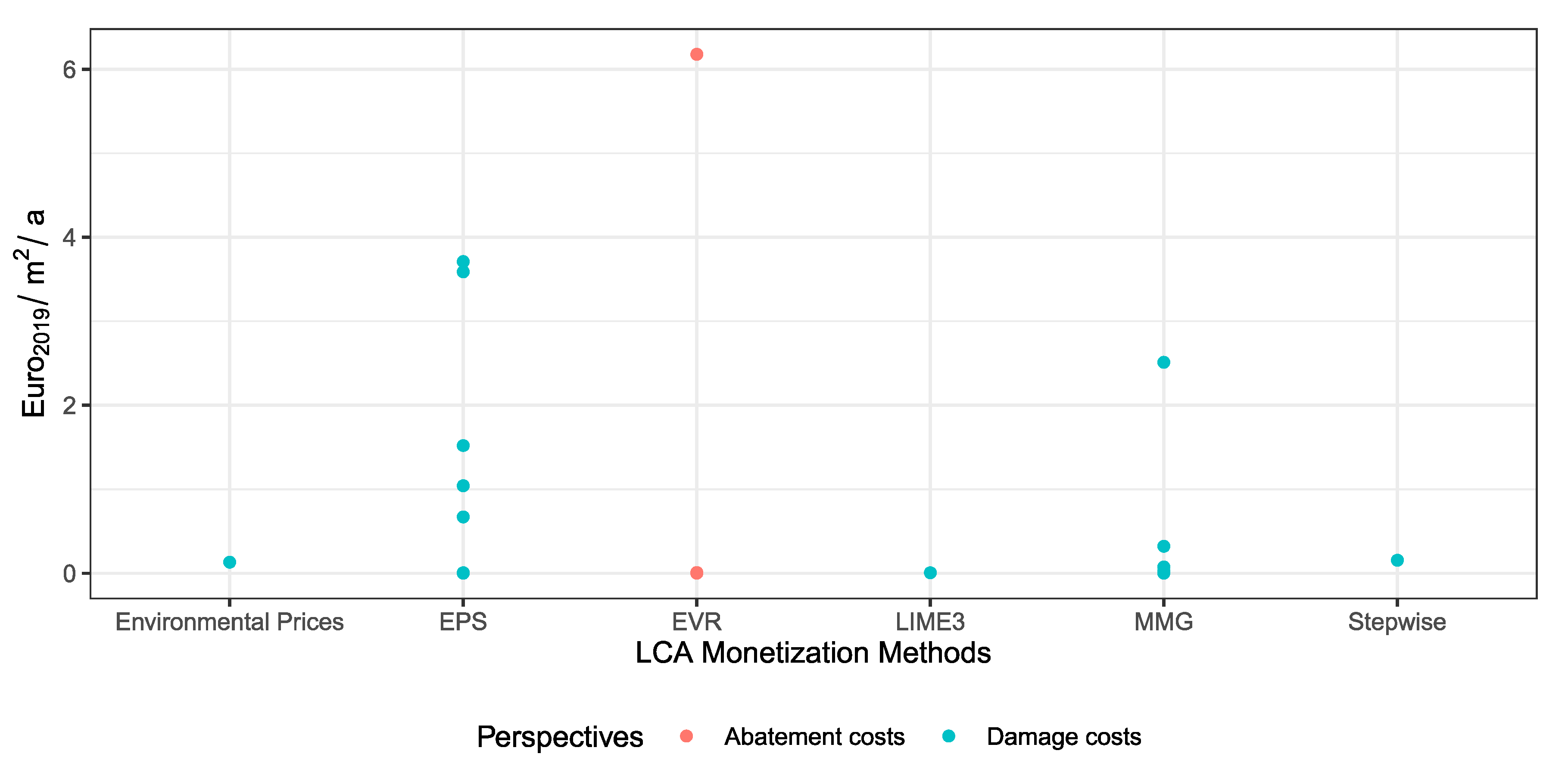
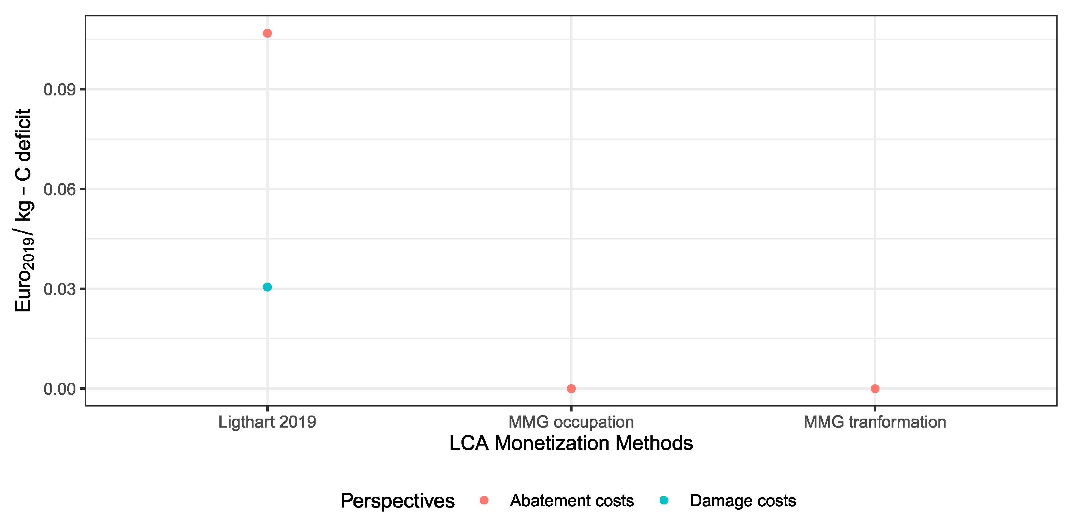
3.3.11. Land Use, Land Transformation and Soil Organic Matter

Six methods assessed the impact category land use, while only two assessed land transformation and two assessed soil organic matter. The values for land use are displayed in Figure 16.

The values for land use range between 6 €/m²/a (heterogeneous agriculture) from EVR to 12 ct for m²/a for Stepwise. However, the values also contain different land use types. We assume that the 6 €/m²/a are a mistake in EVR, because there is no reason why heterogeneous agriculture should have higher eco costs than an artificial area. The calculations in EVR are based on land use for agricultural products from Europe and consider the species richness and the biodiversity factor. EVR does not provide land occupation data for industrial or urban use. For EPS the values for urban and industrial use are the highest (just under 4 €/m²/a), while the agricultural values are an order of magnitude lower than the agricultural values determined by the EVR. The EPS assesses the impact on biodiversity, but also agricultural damages (if an area is an urban area the fact that no wood and vegetables can be produced on it are included as damages- opportunity costs). The EPS also considers the impact on the reduced drinking water renewal rate. The dominant factor of the EPS though are the effect of the urban heat island on working capacity that constitute over 3 €/m²/a. For agricultural land use, the values are very low (0.5 ct) and only quantify biodiversity impacts.

Environmental Prices mainly assess impact on biodiversity. Its provided values are higher than the ones provided by EPS for agricultural use. However, it does not publish the associated environmental costs for all kinds of land use and thus provides the same value for urban and agricultural land use.

The MMG method values the impact on biodiversity based on lost ecosystem services for urban and industrial areas, for agricultural areas they use abatement costs, based on a study by Tucker, that is not listed in the methods references. Stepwise calculates damages to biodiversity and obtains a monetary value similar to the Environmental Prices method.

LIME3 considers impacts of land transformation on biodiversity and NPP and of land occupation on NPP. Due to the data availability, only land occupation impacts are assessed in this study. As most other methods do not consider impacts on NPP, the value is difficult to compare. The value and impact determined by LIME3 to primary production seems lower compared to the impacts on biodiversity in the other methods.

For land use transformation, we only have two methods that deliver data (Environmental Prices does not deliver them as a weighting factor in LCA but for application to other studies. It is 3.26 €₂₀₁₅/m² and assumes a 50-year time horizon of use and a 3% discount rate). The values are displayed in Figure 17.

For the MMG method a value from the TEEB study was adapted that is based on land use change in the tropical rainforest and its annual biodiversity losses. They discounted the losses at 3%. It remains unclear whether these values have been directly transferred to Europe. As the tropical rainforest has a very high biodiversity and bio productivity, this baseline is likely to have increased the values. For EVR the approach and the values for transformation and occupation are the same.

Only two methods provide values for soil organic matter (the MMG method and the method by Ligthart and van Hamelen). The values are both oriented towards the midpoint category that is connected to land use [107,108]. The values are shown in Figure 18.

The MMG method, that delivers lower values, is based on abatement costs and considered the technologies that would be realized if a carbon tax of 100 $/t CO₂ was implemented, e.g., zero tillage. Based on this, they assume costs of 0.00000034 € per kg C. We do not really understand what they calculated here and how they obtained this very low value. If we assumed 100 $/t CO₂ (corresponding to 0.1 $/kg CO₂) the associated value for storing carbon in the ground would be 0.275 $/kg of C. With this value the MMG value would be much higher than the values from Ligthart and van Hamelen [104]. Further, it is unclear to us why different values for soil organic matter for transformation and occupation are delivered.

The study by Ligthart and van Hamelen [104] determined damage and abatement costs of soil organic matter loss. The damage costs only include economic damages to agricultural productivity (yield loss). The abatement costs are based on avoided costs of fertilizer.

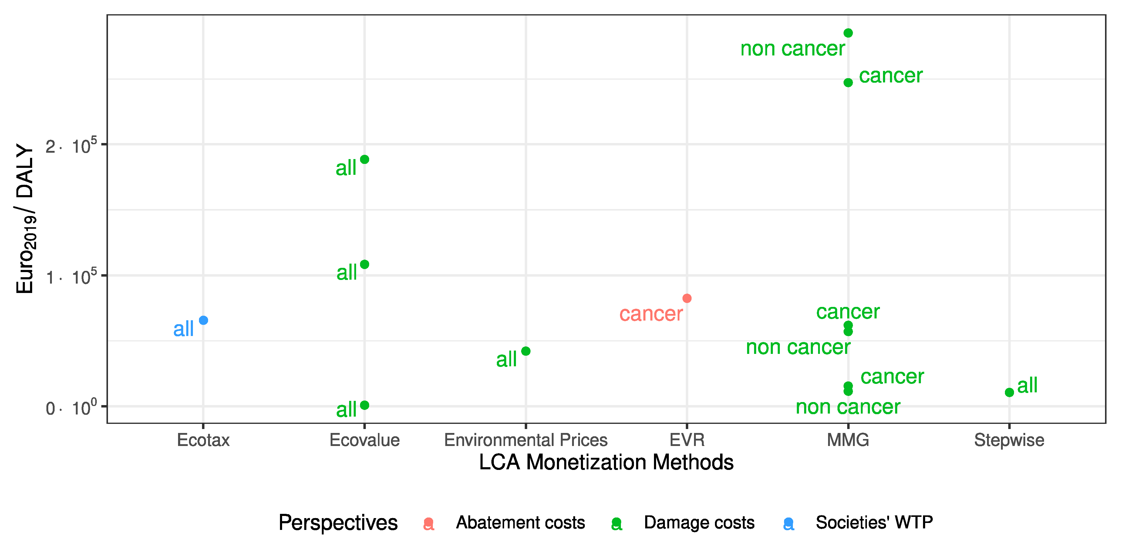
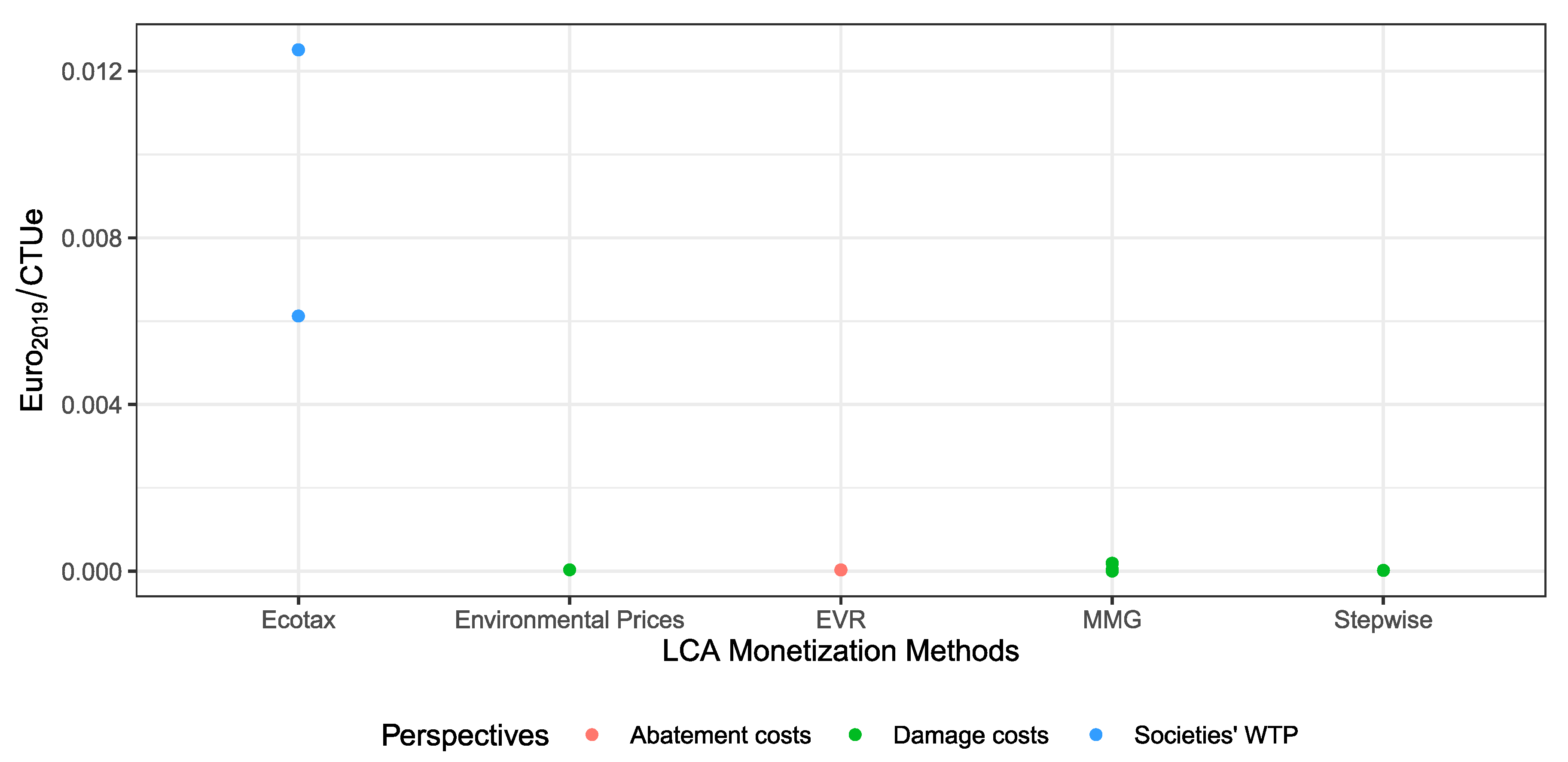
3.3.12. Human Toxicity

Six methods provided monetary values for human toxicity. Their results are visualized in Figure 19.

As we converted the impact of toxic substances to DALY with the USEtox model, it was expected that the €/DALY values would be similar to the value that has been assigned to human health for VOLY based on the NEEDS WTP studies. The values range around these data with the highest value for the MMG high estimate for non-cancer (with 285,156.68 €/DALY) and the lowest value for Ecovalue’s minimum estimate with 771 €/DALY.

MMG includes DALY losses, and for cancer also the costs of cancer treatment and the associated productivity loss [109]. The values for non-cancer have a larger range, because CTUh for non-cancer effects are more uncertain [110].

Another noteworthy observation is that the values for Stepwise are rather low, even though Stepwise has a high valuation of €/DALY (as shown in Table 2). In addition, the cause-effect chain of Stepwise is not based on USEtox but on Impact 2002+. If we use (instead of USEtox characterization factors) first the conversion factor by Pizzol [20] to transfer Vinylchloride (the impact assessment indicator for Stepwise) to convert to 1,4DCB-e to air (0.0057 kg C₂H₃Cl/kg DCB to air) we yield very low values for Stepwise per DALY (~800 €/DALY). This seems much too low. Therefore, these differences must be due to different characterization factors and impact assessment modelling in the toxicity assessments of Impact 2002+ and USEtox, because the valuation of a human life in all assessed methods is in a similar range. Further Stepwise includes damages to resource productivity of humans due to work (Table 13.1 in reference [65]), which all other methods do not include, which is in contrast with the low values obtained here.

For Environmental Prices the valuation is very close to the NEEDS approximation (~42,000 €/DALY), even though it is based on ReCiPe toxicity assessment which seems to not yield very different results compared to USEtox in our assessment. Another rather high value is from EVR (80,000 €) which based on kidney hospital treatment and is an upper bound [111]. The calculation from the emissions back to the DALY yield the same result in our assessment, because our calculations are based on USEtox and the calculations of the EVR are based on USEtox as well. Ecovalue has the highest medium value. According to Finnveden and Noring the value is based on the Shadow Prices Handbook [101], which is also based on NEEDs WTP for life expectancy. If they were income adjusted by Sweden’s GDP, the high value would be partially explainable since the Swedish GDP is higher than the EU’s average, but the exact transfer is not documented. For the Ecotax method the tax is based on cadmium content in fertilizer, which is very high and yields a value of 65.000 € which is close to Swedish GDP per capita.

If we look at the average values and the variance (see Figure 3), we can see that the data is close to normally distributed and we do not have any outliers. Further research is needed to compare the differences in the underlying toxicity assessments and their effect on the different DALY values.

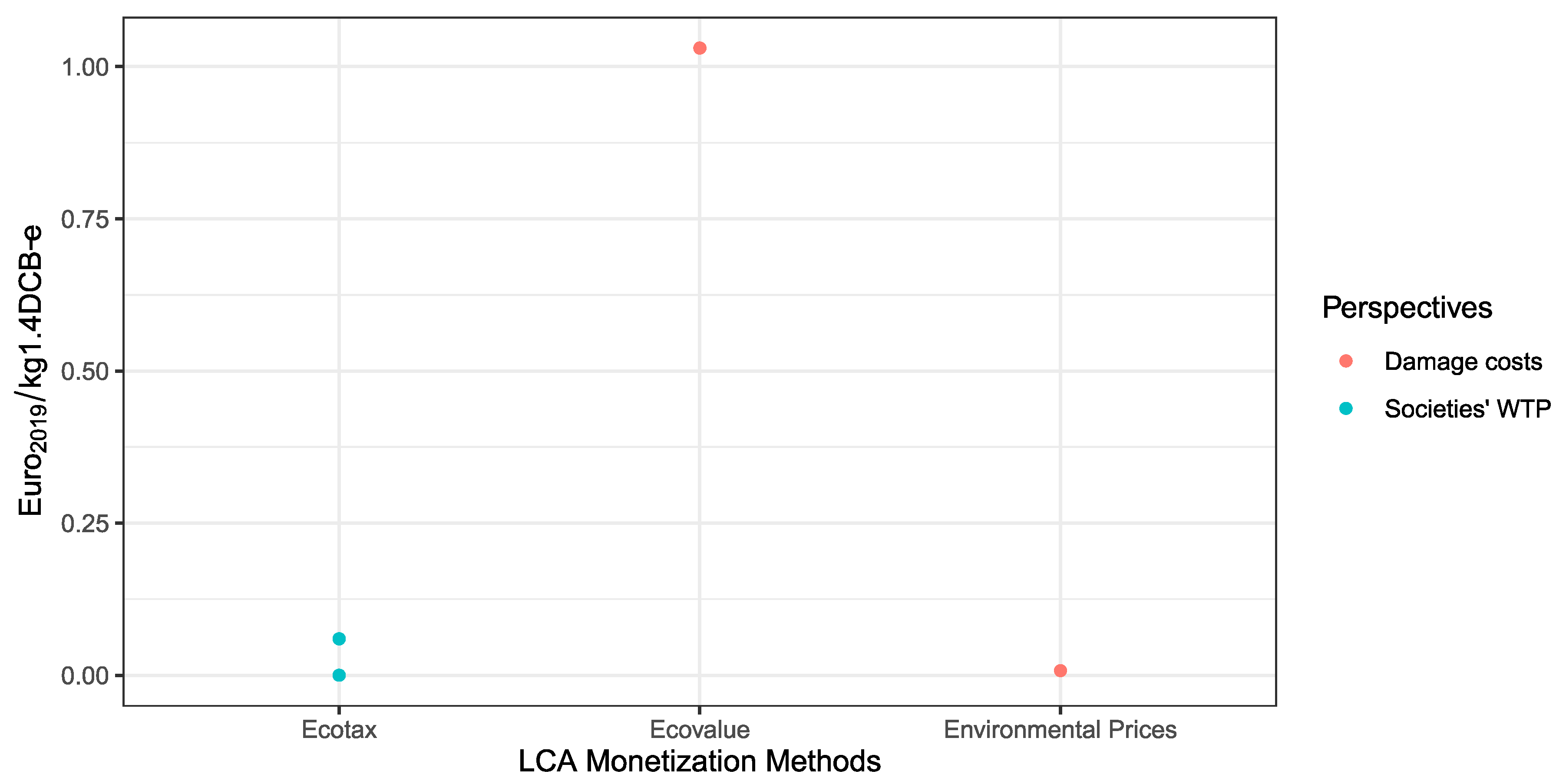
3.3.13. Terrestrial Ecotoxicity

Three methods provide data on terrestrial ecotoxicity, namely Ecotax, Environmental Prices and Stepwise. The values are displayed in Figure 20.

Ecotax has the highest value; it is based on a Swedish tax on exceeding cadmium values in fertilizer. For Environmental Prices ecotoxicity impacts are assessed through ReCiPe 2013 [102] and then monetized by the values provide by Kuik et al. [82], that are higher than most other ecosystem values. It is not clear why Stepwise is so much lower than Environmental Prices, even though its biodiversity valuation delivers higher values than the Environmental Prices medium estimate (see Table 2). The differences must therefore be due to different impact assessment: while Environmental Prices uses ReCiPe, Stepwise uses Impact 2002+ as its impact assessment method.

3.3.14. Freshwater Ecotoxicity

The impact category freshwater ecotoxicity is assessed by five methods (see Figure 21).

Also for this toxicity category, the highest value is provided by the Ecotax method based on toluene emissions to freshwater. EVR costs are based on wastewater treatment to remove toxic substances (lead substance copper). For Environmental Prices, the model is based on ReCiPe and on the species valuation of Kuik et al. [82]. The MMG method is based on USEtox and on the biodiversity valuation of Ott et al. [80]. After Ecotax, the MMG method shows the highest value (high and central estimate). This is surprising because the ecosystem valuation of Ott et al. [80] is lower than the one by Kuik et al. [82]. Accordingly, we would have expected a higher value for Environmental Prices, but apparently the differing impact assessments play a role here. Stepwise values are very low, again presumably due to the different impact assessment used, as for terrestrial ecotoxicity.

3.3.15. Marine Ecotoxicity

For marine ecotoxicity, three methods provide values, namely Ecotax, Ecovalue and Environmental Prices (see Figure 22).

It is worth noticing that the damage costs for Ecovalue are much higher than the societies’ WTP. It is also remarkable that the Ecovalue method and Ecotax both assess impacts in Sweden. The Ecotax method bases its calculation on taxes based on toxic substances in pesticides (copper), which is apparently a lot lower than the associated damages of such an emission. For Environmental Prices the impact modelling is based on ReCiPe 2013 between individualist and hierarchist perspectives and the economic valuation is based on the data by Kuik et al. [82]. For the Ecovalue method, the values are based on a study by Noring et al. [112] on tributyline pollution, but no documentation could be found how the tributylene pollution was transferred to 1,4-DCB equivalents. Even though Noring et al. [112] excluded very high answers, the obtained values are the highest. The value is based on contingent valuation and WTP that was linked to reaching a certain policy target that would increase the environmental status of several snails and other species. Because of the nature of the assessment in Ecovalue (specific pollutant, geographically discrete), it is not surprising that the value is higher.

Only Environmental Prices provides data that have a link to ecosystems, but they also state that their values have limited validation, especially if site-specific studies should be performed.

What is noteworthy is that for freshwater and terrestrial ecotoxicity the values for the Ecotax method deliver the highest values, while it provides lower values for marine ecotoxicity. This inconsistency in the Ecotax method occurs presumably because the Ecotax method has no underlying link to any AoP.

4. Discussion

Within the quantitative comparison, the most important uncertainties are unrelated to the adjustment of the monetary values for inflation and currency. The process of harmonizing the different impact category (methods and) indicators prior to comparing the weighted results involves the most severe uncertainties (i.e., the unit conversion factors documented in Table S1). The same uncertainty applies to the conversion of the EU normalization factors per capita. Time did not allow us to analyze the influence of different unit conversion factors, that are based on various impact assessment methods, on the results. The conversion factors have a big impact if some methods do not link impacts clearly to an AoP such as the Ecotax method, or if they do not convert environmental releases or extraction of resources to an impact category indicator (as in the EPS or EVR for mineral resources). These methods often monetized impacts at the inventory level. The comparison of the impacts for some impact categories such as the toxicity impacts and the use of mineral resources should be interpreted with great care: As some values that we compared here do not have a common impact assessment, a comparison by substance or by material would be necessary to obtain a more meaningful result. This would allow one to compare how the impact of different substances and materials are valued in more detail and not only for 1,4-DCB-e or Sb-e for the toxicity and mineral resources respectively. Therefore, the monetary factors in Table S3 in the supplementary materials for these impact categories should not be used as weighting factors, as the monetization methods themselves partially do not use an impact assessment but monetize at inventory level (e.g., the EPS or EVR), or use different underlying impact assessments (e.g., USEtox or ReCiPe).

For many impact categories, the main influencing factor could be identified (i.e., differences in the impact assessment, the evaluated AoP or its valuation). For others, however, this was not possible. For the monetization of the impact category freshwater ecotoxicity regarding the MMG method and Environmental prices, for example, the valuation of the AoPs was known and suggested a higher value for Environmental prices for biodiversity, but the obtained values for freshwater ecotoxicity were still higher for the MMG method. Within the scope of this research, it was not possible to separate those two influencing factors (the impact assessment and the AoP valuation). A more in-depth analysis of individual impact categories that explicitly compares different impact assessment methods and monetization of the associated environmental impact would be needed.

Within the qualitative assessment, the geographical scope has been shown to considerably change the magnitude of the results. Compared to the other qualitative characteristics the values were highest if the reference region was rich. This aspect was even more dominant than the chosen discount rate or, if applied, equity weighting (even though choosing an LCA monetary valuation method derived in a rich geographical region to a poorer region can also be perceived as a kind of equity weighting). The relevance of the geographical scope underscores that there is a trade-off between universal applicability and global monetization methods on the one hand, and a site dependent and much more meaningful result on the other. As impact assessment methods are becoming more regionalized, the monetary valuation of associated impacts should also be region specific, to deliver more meaningful results. To calculate the influence of the geographical scope, benefit transfer methods can be used as applied in Ahlroth et al. [63]. But these models need to be applied with caution as valuation of non-marketed goods is often culturally diverse beyond income [113]. Therefore, practitioners that want to monetize their LCA results should pay attention to where the lion’s share of the environmental burden occurs and should choose the monetization methods accordingly.

The inclusion of different AoPs varies for the different methods. In environmental economics it is common practice to include damages to crops and working productivity and human wellbeing but these are not universally accepted AoPs in environmental LCA. The differing included AoPs for nearly all impact categories from ReCiPe [26] and Environmental Prices [29], but also for other methods underscore this problem. This aspect can be highlighted regarding the impact category water: are its damages covered sufficiently by damages to ecosystems and induced malnutrition, or should forgone income of farmers due to reduced yields be included as well? Therefore, a further research objective is to clarify the relation of environmental LCA to welfare and environmental economics.

Because many methods do not establish a link to all damaged AoPs (e.g., the link from water use to ecosystems), it can safely be stated that most monetary damage factors merely represent a lower bound. One of the biggest challenges is to monetize biodiversity and ecosystem services. The link between ecosystem services and LCA is mainly established by the Trucost method. A comparison of its biodiversity valuation with that of other methods is precluded because the underlying calculations are not disclosed. Apart from the Trucost method, only a limited number of studies were used to value biodiversity [76,80,81,82]. This again underlines the need to better integrate research on ecosystem services and environmental economics with LCA. Currently, all other monetization methods in LCA studies assessing biodiversity only include effects on limited amounts of species (vascular plants or birds) as the studies by the NEEDS project [80,82], the study for EPS [81] and the study in LIME3 [69].

Even if the uncertainties in the unit conversion factors and the different geographical scopes were negligible, we doubt that the values would converge significantly. In the last step of the quantitative comparison, it became visible that the monetization methods prioritize different impact categories. The weight assigned to the different impact categories when they were applied to environmental damages of an average EU citizen varied for many impact categories: climate change (7% to 58%), mineral resources (0% to 32%), particulate matter (5% to 35%) and POCP (0 to 82%). Therefore, it is expected that the choice of the monetization method leads to different recommendations regarding product optimization or consumption choices (see Figure 4). If a practitioner wanted to pay specific attention to global warming and assigning ~50% of total human damages seemed right to them, the Ecovalue or Stepwise might be the right choice. If another practitioner was particularly concerned with mineral and fossil resources, LIME3 or EPS would be more in line with their worldview. Additionally, practitioners could apply several monetization methods to their case study in order to verify whether results, such as the superiority of one product over another (in terms of their environmental LCA results) or an identified significant process, are sensitive to the applied monetization method. They should also pay attention to the covered impact categories: a monetization method that does not supply monetary values for land use and energy should not be applied to a study that compares bioenergy with fossil energy, as it will undervalue the impact of bioenergy.

The calculated environmental damages of the damage of an average EU citizen should be interpreted with care: these factors only include domestic environmental impacts and no emissions embedded in trade. If these were included, the damages would rise. The calculation was mainly performed for illustrative purposes to obtain information how the monetization methods weight in between midpoints.

We derive from our results that the monetary weighting of LCA results will benefit from further research and discussion in the field, potentially leading to results that are more meaningful and accepted by a wide scientific community. The information for monetary valuation in the Annex C of the ISO standard for monetary valuation [42], especially Table 2, should be considered by method developers in their choices which underlying valuation studies to choose to value AoPs. Further, standards for good practice in the field of stated preference studies in general and choice modelling in particular [114] should be considered by the LCA monetization community (e.g., attributes of one particular good are traded rather than different goods among themselves). Moreover, advances in participatory valuation in the field of ecosystem services [115] might be interesting for LCA. Furthermore, WTA studies could be used for monetization in LCA to see how the magnitude of the valuation would change if the property rights of the welfare loss associated with the emissions and resources use was assigned to the entity whose welfare is reduced. If the monetary values obtained by WTP studies are used to estimate the amount that the entity whose welfare is reduced by the pollution or resources use should be compensated for, in order to be equally well as before the caused environmental harm, the use of WTP will result in a loss [116]. For that purpose WTA, values would be more adequate.

Availability of information was an issue in the evaluation of some methods. While the documentation of the calculations for the EPS method, EVR, MMG and Environmental Prices was thorough and clear, this was different for the other methods. The extreme end of this was the Trucost method, whose naming is definitely misleading as we are far from a “Trucost” in monetizing LCA results, that did not disclose any calculations. To enable a constant improvement of methods, results and calculations should be documented in detail.

5. Conclusions

This study provided an overview of currently applied monetization methods in LCA. Values from nine methods covering 18 impact categories were compared qualitatively and quantitatively. The quantitative results show a non-normal distribution of the obtained damage factors for the different impact categories. Additionally, the methods emphasize the various impact categories quite differently, showing different preference structures. The most influential criterion was the geographical reference area (i.e., the richer the reference area, the higher the results). Choosing the discount rate and equity weighting turned out to be less important. Overall, we can state that current monetization methods in LCA use a wide variety of monetary valuation approaches. Therefore, varying monetary damage values are obtained. Practitioners should especially pay attention to the coherence of the underlying reference region of monetization methods and their case study. Method developers, in turn, should concentrate on the quality of the valuation studies from which they derive their monetary values. For some impact categories, mainly those concerned with impacts on human health, the monetary values converge more than for others. This is attributed to the fact that valuing the AoP human health is more developed than valuing biodiversity and resources. One of the major identified weaknesses is the valuation of biodiversity, which is currently mainly oriented to valuation of vascular plants in LCA. Monetized LCIA results related to biodiversity and resources show wide ranges and a non-normal distribution. Further consensus is needed on which kind of damages should be included in the AoPs. For example, there is no consensus on whether reduced labor productivity or damages to assets such as buildings should be included. Further, no monetization method for LCA is available that uses WTA.

References

1. Boardman, A.; Greenberg, D.; Vining, A.; Weimer, D. Cost Benefit Analysis: Concepts and Practice; Cambridge University Press: Cambridge, UK, 2018. [Google Scholar]
2. Wolff, F.; Gsell, M. Ökonomisierung der Umwelt und Ihres Schutzes: Unterschiedliche Praktiken, Ihre Theoretische Bewertung und Empirische Wirkungen; German Federal Environmental Agency: Berlin/Dessau, Germany, 2018. [Google Scholar]
3. Bachmann, T.M. Considering environmental costs of greenhouse gas emissions for setting a CO2 tax: A review. Sci. Total Environ. 2020, 720, 137524. [Google Scholar] [CrossRef] [PubMed]
4. Kylili, A.; Fokaides, P.A.; Ioannides, A.; Kalogirou, S. Environmental assessment of solar thermal systems for the industrial sector. J. Clean. Prod. 2018, 176, 99–109. [Google Scholar] [CrossRef]
5. Walker, S.B.; Fowler, M.; Ahmadi, L. Comparative life cycle assessment of power-to-gas generation of hydrogen with a dynamic emissions factor for fuel cell vehicles. J. Energy Storage 2015, 4, 62–73. [Google Scholar] [CrossRef]
6. Bachmann, T.M. Optimal pollution: The welfare economic approach to correct related market failures. In Encyclopedia of Environmental Health; Elsevier: Amsterdam, The Netherlands, 2019; Volume 4, pp. 767–777. ISBN 9780444639523. [Google Scholar]
7. Pizzol, M.; Laurent, A.; Sala, S.; Weidema, B.; Verones, F.; Koffler, C. Normalisation and weighting in life cycle assessment: Quo vadis? Int. J. Life Cycle Assess. 2017, 22, 853–866. [Google Scholar] [CrossRef] [Green Version]
8. Rauner, S.; Bauer, N.; Dirnaichner, A.; Van Dingenen, R.; Mutel, C.; Luderer, G. Coal-exit health and environmental damage reductions outweigh economic impacts. Nat. Clim. Chang. 2020, 10, 308–312. [Google Scholar] [CrossRef] [Green Version]
9. Schneider-Marin, P.; Lang, W. Environmental costs of buildings: Monetary valuation of ecological indicators for the building industry. Int. J. Life Cycle Assess. 2020, 25, 1637–1659. [Google Scholar] [CrossRef]
10. ISO. ISO 14040: Environmental Management–Life Cycle Assessment—Principles and Framework; ISO: Geneva, Switzerland, 2006. [Google Scholar]
11. ISO. ISO 14044:2006 Environmental Management—Life Cycle Assessement—Requirements and Guidelines; ISO: Geneva, Switzerland, 2006. [Google Scholar]
12. Steen, B.; Ryding, S.O. The EPS Enviro-Accounting Method; Swedish Environmental Research Institute (IVL): Göteborg, Sweden, 1992. [Google Scholar]
13. Inaba, A.; Itsubo, N. Preface. Int. J. Life Cycle Assess. 2018, 23, 2271–2275. [Google Scholar] [CrossRef] [Green Version]
14. Itsubo, N.; Inaba, A. A new LCIA method: LIME has been completed. Int. J. Life Cycle Assess. 2003, 8, 305. [Google Scholar] [CrossRef]
15. Itsubo, N.; Sakagami, M.; Kuriyama, K.; Inaba, A. Statistical analysis for the development of national average weighting factors-visualization of the variability between each individual’s environmental thought. Int. J. Life Cycle Assess. 2012, 17, 488–498. [Google Scholar] [CrossRef]
16. Vogtländer, J.G.; Brezet, H.C.; Hendriks, C.F. The virtual eco-costs ‘99 A single LCA-based indicator for sustainability and the eco-costs-value ratio (EVR) model for economic allocation. Int. J. Life Cycle Assess. 2001, 6, 157–166. [Google Scholar] [CrossRef]
17. Finnveden, G. A Critical Review of Operational Valuation/Weighting Methods for Life Cycle Assessment; Swedish Environmental Protection Agency: Stockholm, Sweden, 1999. [Google Scholar]
18. Finnveden, G.; Eldh, P.; Johansson, J. Weighting in LCA based on ecotaxes: Development of a mid-point method and experiences from case studies. Int. J. Life Cycle Assess. 2006, 11, 81–88. [Google Scholar]
19. Ferreira, S.; Cabral, M.; Da Cruz, N.F.; Marques, R.C. Economic and environmental impacts of the recycling system in Portugal. J. Clean. Prod. 2014, 79, 219–230. [Google Scholar] [CrossRef]
20. Pizzol, M.; Weidema, B.; Brandão, M.; Osset, P. Monetary valuation in Life Cycle Assessment: A review. J. Clean. Prod. 2015, 86, 170–179. [Google Scholar] [CrossRef]
21. Dong, Y.; Hauschild, M.; Sørup, H.; Rousselet, R.; Fantke, P. Evaluating the monetary values of greenhouse gases emissions in life cycle impact assessment. J. Clean. Prod. 2019, 209, 538–549. [Google Scholar] [CrossRef]
22. Durao, V.; Silvestre, J.D.; Mateus, R.; De Brito, J. Economic valuation of life cycle environmental impacts of construction products—A critical analysis. IOP Conf. Ser. Earth Environ. Sci. 2019, 323. [Google Scholar] [CrossRef]
23. Hanley, N.; Spash, C.L. Cost-Benefit Analysis and the Environment; Edward Elgar Publishing Company: Cheltenham, UK, 1993; ISBN 1852784555. [Google Scholar]
24. Horowitz, J.K.; McConnell, K.E. Willingness to accept, willingness to pay and the income effect. J. Econ. Behav. Organ. 2003. [Google Scholar] [CrossRef] [Green Version]
25. Isoni, A. The willingness-to-accept/willingness-to-pay disparity in repeated markets: Loss aversion or “bad-deal” aversion? Theory Decis. 2011. [Google Scholar] [CrossRef] [Green Version]
26. Huijbregts, M.A.J.; Steinmann, Z.J.N.; Elshout, P.M.F.; Stam, G.; Verones, F.; Vieira, M.; Zijp, M.; Hollander, A.; van Zelm, R. ReCiPe2016: A harmonised life cycle impact assessment method at midpoint and endpoint level. Int. J. Life Cycle Assess. 2017, 22, 138–147. [Google Scholar] [CrossRef]
27. Itsubo, N.; Murakami, K.; Kuriyama, K.; Yoshida, K.; Tokimatsu, K.; Inaba, A. Development of weighting factors for G20 countries—Explore the difference in environmental awareness between developed and emerging countries. Int. J. Life Cycle Assess. 2018, 23, 2311–2326. [Google Scholar] [CrossRef] [Green Version]
28. Steen, B. Calculation of Monetary Values of Environmental Impacts from Emissions and Resource Use The Case of Using the EPS 2015d Impact Assessment Method. J. Sustain. Dev. 2016, 9, 15. [Google Scholar] [CrossRef] [Green Version]
29. De Bruyn, S.; Bijleveld, M.; de Graaff, L.; Schep, E.; Schroten, A.; Vergeer, R.; Ahdour, S. Environmental Prices Handbook; CE Delft: Delft, The Netherlands, 2018. [Google Scholar]
30. Anthoff, D.; Hepburn, C.; Tol, R.S.J. Equity weighting and the marginal damage costs of climate change. Ecol. Econ. 2009, 68, 836–849. [Google Scholar] [CrossRef] [Green Version]
31. Hellweg, S.; Hofstetter, T.B.; Hungerbühler, K. Discounting and the environment should current impacts be weighted differently than impacts harming future generations? Int. J. Life Cycle Assess. 2003, 8, 8. [Google Scholar] [CrossRef]
32. Nordhaus, W.D. A review of the Stern Review on the economics of climate change. J. Econ. Lit. 2007, 45, 686–702. [Google Scholar] [CrossRef]
33. Stern, N. Stern Review: The Economics of Climate Change; Cambridge University Press: Cambridge, UK, 2006. [Google Scholar] [CrossRef]
34. Albertí, J.; Balaguera, A.; Brodhag, C.; Fullana-i-Palmer, P. Towards life cycle sustainability assessent of cities. A review of background knowledge. Sci. Total Environ. 2017, 609, 1049–1063. [Google Scholar] [CrossRef] [PubMed]
35. Cremer, A.; Müller, K.; Berger, M.; Finkbeiner, M. A framework for environmental decision support in cities incorporating organizational LCA. Int. J. Life Cycle Assess. 2020, 25, 2204–2216. [Google Scholar] [CrossRef]
36. Loiseau, E.; Aissani, L.; Le Féon, S.; Laurent, F.; Cerceau, J.; Sala, S.; Roux, P. Territorial Life Cycle Assessment (LCA): What exactly is it about? A proposal towards using a common terminology and a research agenda. J. Clean. Prod. 2018, 176, 474–485. [Google Scholar] [CrossRef] [Green Version]
37. Martínez-Blanco, J.; Finkbeiner, M. Organisational LCA. In Life Cycle Assessment: Theory and Practice; Springer International Publishing: Basel, Switzerland, 2017; ISBN 9783319564753. [Google Scholar]
38. Boulay, A.M.; Benini, L.; Sala, S. Marginal and non-marginal approaches in characterization: How context and scale affect the selection of an adequate characterization model. The AWARE model example. Int. J. Life Cycle Assess. 2019, 1–13. [Google Scholar] [CrossRef]
39. Forin, S.; Berger, M.; Finkbeiner, M. Comment to “Marginal and non-marginal approaches in characterization: How context and scale affect the selection of an adequate characterization factor. The AWARE model example.” Int. J. Life Cycle Assess. 2020, 25, 663–666. [Google Scholar] [CrossRef]
40. Nicholson, W.; Snyder, C. Intermediate Microeconomics and Its Application; South-Western College Publishing: Cincinnati, OH, USA, 2009; ISBN 9781439044049. [Google Scholar]
41. Revesz, R.L.; Howard, P.H.; Arrow, K.; Goulder, L.H.; Kopp, R.E.; Livermore, M.A.; Oppenheimer, M.; Sterner, T. Global warming: Improve economic models of climate change. Nature 2014, 508, 173. [Google Scholar] [CrossRef]
42. ISO. ISO 14008:2019 Monetary Valuation of Environmental Impacts and Related Environmental Aspects; ISO: Geneva, Switzerland, 2019. [Google Scholar]
43. Thompson, G. Statistical Literacy Guide: How to Adjust for Inflation; House of Commons Library: London, UK, 2009; pp. 1–6. [Google Scholar]
44. Eurostat HICP (2015=100)—Annual Data (Average Index and Rate of Change). Available online: https://ec.europa.eu/eurostat/web/hicp/data/database (accessed on 16 August 2020).
45. Statistiska Centralbyrån (SCB) CPI, Fixed Index Numbers (1980=100). Available online: https://www.scb.se/en/finding-statistics/statistics-by-subject-area/prices-and-consumption/consumer-price-index/consumer-price-index-cpi/pong/tables-and-graphs/consumer-price-index-cpi/cpi-fixed-index-numbers-1980100/ (accessed on 16 August 2020).
46. U.S. Bureau of Labor Statistics Consumer Price Index Historical Tables for U.S. City Average. Available online: https://www.bls.gov/regions/mid-atlantic/data/consumerpriceindexhistorical_us_table.htm (accessed on 16 August 2020).
47. OECD Purchasing Power Parities (PPP). Available online: https://data.oecd.org/conversion/purchasing-power-parities-ppp.htm (accessed on 16 August 2020).
48. Owsianiak, M.; Laurent, A.; Bjørn, A.; Hauschild, M.Z. IMPACT 2002+, ReCiPe 2008 and ILCD’s recommended practice for characterization modelling in life cycle impact assessment: A case study-based comparison. Int. J. Life Cycle Assess. 2014, 19, 1007–1021. [Google Scholar] [CrossRef]
49. Dreyer, L.C.; Niemann, A.L.; Hauschild, M.Z. Comparison of three different LCIA methods: EDIP97, CML2001 and eco-indicator 99: Does it matter which one you choose? Int. J. Life Cycle Assess. 2003, 8, 191–200. [Google Scholar] [CrossRef]
50. Frischknecht, R.; Steiner, R.; Jungbluth, N. The Ecological Scarcity Method—Eco-Factors 2006. A Method for Impact Assessment in LCA; Federal Office for the Environment FOEN: Bern, Switzerland, 2009. [Google Scholar]
51. Fantke, P.; Bijster, M.; Guignard, C.; Hauschild, M.; Huijbregts, M.; Jolliet, O.; Kounina, A.; Magaud, V.; Margni, M.; McKone, T.E.; et al. USEtox®2.0 Documentation (Version 1); Technical University of Denmark (DTU): Lyngby, Denmark, 2017. [Google Scholar]
52. Jolliet, O.; Margni, M.; Charles, R.; Humbert, S.; Payet, J.; Rebitzer, G.; Rosenbaum, R. IMPACT 2002+: A New Life Cycle Impact Assessment Methodology. Int. J. Life Cycle Assess. 2003, 8, 324. [Google Scholar] [CrossRef] [Green Version]
53. Posch, M.; Seppälä, J.; Hettelingh, J.P.; Johansson, M.; Margni, M.; Jolliet, O. The role of atmospheric dispersion models and ecosystem sensitivity in the determination of characterisation factors for acidifying and eutrophying emissions in LCIA. Int. J. Life Cycle Assess. 2008, 13, 477. [Google Scholar] [CrossRef]
54. Bare, J. TRACI 2.0: The tool for the reduction and assessment of chemical and other environmental impacts 2.0. Clean Technol. Environ. Policy 2011, 13, 687–696. [Google Scholar] [CrossRef]
55. World Nuclear Association Heat Values of Various Fuels. Available online: https://www.world-nuclear.org/information-library/facts-and-figures/heat-values-of-various-fuels.aspx (accessed on 14 November 2020).
56. Huijbregts, M.A.J.; Rombouts, L.J.A.; Ragas, A.M.; van de Meent, D. Human-toxicological effect and damage factors of carcinogenic and noncarcinogenic chemicals for life cycle impact assessment. Integr. Environ. Assess. Manag. 2005, 1, 181–244. [Google Scholar] [CrossRef]
57. Benini, L.; Mancini, L.; Sala, S.; Schau, E.; Manfredi, S.; Pant, R. Normalisation Method and Data for Environmental Footprints; Publications Office of the European Union: Luxembourg, 2014; ISBN 9789279408472. [Google Scholar]
58. Sala, S.; Crenna, E.; Secchi, M.; Pant, R. Global Normalisation Factors for the Environmental Footprint and Life Cycle Assessment; Publications Office of the European Union: Luxembourg, 2017. [Google Scholar] [CrossRef]
59. Ahlroth, S.; Finnveden, G. Ecovalue08—A new valuation set for environmental systems analysis tools. J. Clean. Prod. 2011, 19, 1994–2003. [Google Scholar] [CrossRef]
60. Ahlroth, S. Valuation of Environmental Impacts and Its Use in Environmental Systems Analysis Tools; KTH Royal Institute of Technology: Stockholm, Sweden, 2009. [Google Scholar]
61. Noring, M. Valuing Ecosystem Services: Linking Ecology and Policy; KTH Royal Institute of Technology: Stockholm, Sweden, 2014. [Google Scholar]
62. Finnveden, G.; Noring, M. A new set of valuation factors for LCA and LCC based on damage costs: Ecovalue 2012. In Proceedings of the 6th International Conference on Life Cycle Management: Perspectives on Managing Life Cycles, Gothenburg, Sweden, 25–28 August 2013; pp. 197–200, ISBN 978-91-980973-5-1. [Google Scholar]
63. Ahlroth, S. Developing a Weighting Set Based on Monetary Damage Estimates. Method and Case Studies; US AB: Stockholm, Sweden, 2009. [Google Scholar]
64. Weidema, B.P. Using the budget constraint to monetarise impact assessment results. Ecol. Econ. 2009, 68, 1591–1598. [Google Scholar] [CrossRef]
65. Weidema, B.P.; Wesnae, M.; Hermansen, J.; Kristensen, I.; Halberg, N. Environmental Improvement Potentials of Meat and Dairy Products; Publications Office of the European Union: Luxembourg, 2008; Volume 23491, ISBN 9789279097164. [Google Scholar]
66. Motoshita, M.; Ono, Y.; Pfister, S.; Boulay, A.M.; Berger, M.; Nansai, K.; Tahara, K.; Itsubo, N.; Inaba, A. Consistent characterisation factors at midpoint and endpoint relevant to agricultural water scarcity arising from freshwater consumption. Int. J. Life Cycle Assess. 2018, 23, 2276–2287. [Google Scholar] [CrossRef] [Green Version]
67. Tang, L.; Nagashima, T.; Hasegawa, K.; Ohara, T.; Sudo, K.; Itsubo, N. Development of human health damage factors for PM2.5 based on a global chemical transport model. Int. J. Life Cycle Assess. 2018, 23, 2300–2310. [Google Scholar] [CrossRef]
68. Tang, L.; Ii, R.; Tokimatsu, K.; Itsubo, N. Development of human health damage factors related to CO2 emissions by considering future socioeconomic scenarios. Int. J. Life Cycle Assess. 2018, 23, 2288–2299. [Google Scholar] [CrossRef]
69. Yamaguchi, K.; Ii, R.; Itsubo, N. Ecosystem damage assessment of land transformation using species loss. Int. J. Life Cycle Assess. 2018, 23, 2327–2338. [Google Scholar] [CrossRef]
70. Vogtländer, J.G. The Model of the Eco-costs/Value Ratio (EVR). Available online: https://www.ecocostsvalue.com/index.html (accessed on 17 September 2020).
71. Vogtländer, J.; Peck, D.; Kurowicka, D. The eco-costs of material scarcity, a resource indicator for LCA, derived from a statistical analysis on excessive price peaks. Sustainability 2019, 11, 2446. [Google Scholar] [CrossRef] [Green Version]
72. Allacker, K.; Trigaux, D.; De Troyer, F. An approach for handling environmental and economic conflicts in the context of sustainable building. WIT Trans. Ecol. Environ. 2014, 181, 79–90. [Google Scholar] [CrossRef] [Green Version]
73. Allacker, K.; De Nocker, L. An Approach for Calculating the Environmental External Costs of the Belgian Building Sector. J. Ind. Ecol. 2012, 16, 710–721. [Google Scholar] [CrossRef]
74. Debacker, W.; Allacker, K.; Spirinckx, C.; Geerken, T.; De Troyer, F. Identification of environmental and financial cost efficient heating and ventilation services for a typical residential building in Belgium. J. Clean. Prod. 2013, 57, 188–199. [Google Scholar] [CrossRef]
75. De Nocker, L.; Debacker, W. Annex: Monetisation of the MMG Method (Update 2017); Public Waste Agency of Flanders (OVAM): Mechele, Belgium, 2018. [Google Scholar]
76. De Groot, R.; Brander, L.; van der Ploeg, S.; Costanza, R.; Bernard, F.; Braat, L.; Christie, M.; Crossman, N.; Ghermandi, A.; Hein, L.; et al. Global estimates of the value of ecosystems and their services in monetary units. Ecosyst. Serv. 2012. [Google Scholar] [CrossRef]
77. Desaigues, B.; Rabl, A.; Chilton, S.; Hugh Metcalf, A.H.; Ortiz, R.; Navrud, S.; Kaderjak, P.; Szántó, R.; Nielsen, J.S.; Jeanrenaud, C.; et al. Final Report on the Monetary Valuation of Mortality and Morbidity Risks from Air Pollution; Université Paris I: Paris, France, 2006. [Google Scholar]
78. Trucost Trucost’s Valuation Methodology. Available online: https://www.gabi-software.com/fileadmin/GaBi_Databases/Thinkstep_Trucost_NCA_factors_methodology_report.pdf (accessed on 8 December 2020).
79. Desaigues, B.; Ami, D.; Bartczak, A.; Braun-Kohlová, M.; Chilton, S.; Czajkowski, M.; Farreras, V.; Hunt, A.; Hutchison, M.; Jeanrenaud, C.; et al. Economic valuation of air pollution mortality: A 9-country contingent valuation survey of value of a life year (VOLY). Ecol. Indic. 2011, 11, 902–910. [Google Scholar] [CrossRef]
80. Ott, W.; Baur, M.; Kaufmann, Y.; Frischknecht, R.; Steiner, R. NEEDS Deliverable D.4.2-RS 1b/WP4—July 06 “Assessment of Biodiversity Losses”. Available online: http://www.needs-project.org/RS1b/RS1b_D4.2.pdf (accessed on 14 December 2020).
81. Mccarthy, D.P.; Donald, P.F.; Scharlemann, J.P.W.; Buchanan, G.M.; Balmford, A.; Green, J.M.H.; Bennun, L.A.; Burgess, N.D.; Fishpool, L.D.C.; Garnett, S.T.; et al. Financial Costs of Meeting Global Biodiversity Conservation Targets: Current Spending and Unmet Needs. Science 2012, 338, 946–949. [Google Scholar] [CrossRef]
82. Kuik, O.; Brander, L.; Nikitina, N.; Navrud, S.; Magnussen, K.; Fall, E.H. Report on the Monetary Valuation of Energy Related Impacts on Land Use, D.3.2. CASES Cost Assessment of Sustainable Energy Systems; University of Amsterdam: Amsterdam, The Netherlands, 2008. [Google Scholar]
83. Preiss, P.; Friedrich, R.; Klotz, V. Deliverable n° 1.1 - RS 3a “Report on the Procedure and Data to Generate Averaged/Aggregated Data”; University of Stuttgart: Stuttgart, Germany, 2008. [Google Scholar]
84. Espreme Estimation of Willingness-To-Pay to Reduce Risks of Exposure to Heavy Metals and Cost-Benefit Analysis for Reducing Heavy Metals Occurrence in Europe. Available online: http://espreme.ier.uni-stuttgart.de (accessed on 14 December 2020).
85. Costanza, R.; D’Arge, R.; De Groot, R.; Farber, S.; Grasso, M.; Hannon, B.; Limburg, K.; Naeem, S.; O’Neill, R.V.; Paruelo, J.; et al. The value of the world’s ecosystem services and natural capital. Nature 1997. [Google Scholar] [CrossRef]
86. Fleurbaey, M.; Zuber, S. Climate Policies Deserve a Negative Discount Rate. Chic. J. Int. Law 2013, 13, 14–15. [Google Scholar]
87. Nordhaus, W.D. Revisiting the social cost of carbon. Proc. Natl. Acad. Sci. USA 2017, 114, 1518–1523. [Google Scholar] [CrossRef] [PubMed] [Green Version]
88. Tol, R.S.J. The Social Cost of Carbon: Trends, Outliers and Catastrophes. Assess. E J. 2008. [Google Scholar] [CrossRef] [Green Version]
89. Ackerman, F.; Stanton, E.A. Climate risks and carbon prices: Revising the social cost of carbon. Economics 2012, 6, 10. [Google Scholar] [CrossRef] [Green Version]
90. Anthoff, D.; Tol, R.S.J.; Yohe, G.W. Risk aversion, time preference, and the social cost of carbon. Environ. Res. Lett. 2009, 4, 024002. [Google Scholar] [CrossRef]
91. Wouter Botzen, W.J.; van den Bergh, J.C.J.M. How sensitive is Nordhaus to Weitzman? Climate policy in DICE with an alternative damage function. Econ. Lett. 2012, 117, 372–374. [Google Scholar] [CrossRef]
92. Tol, R.S.J. The economic impact of climate change. Perspektiven der Wirtschaftspolitik 2010, 11. [Google Scholar] [CrossRef] [Green Version]
93. ISO. ISO 14067:2018 Greenhouse Gases—Carbon Footprint of Products—Requirements and Guidelines for Quantification; ISO: Geneva, Switzerland, 2018. [Google Scholar]
94. Goedkoop, M.; Heijungs, R.; Huijbregts, M.; De Schryver, A.; Struijs, J.; Van Zelm, R. ReCiPe 2008—A life Cycle Impact Assessment Method Which Comprises Harmonised Category Indicators at the Midpoint and the Endpoint Level; Ministry of Housing, Spatial Planning and the Environment (VROM): The Hague, The Netherlands, 2008. [Google Scholar]
95. Methodex BeTa e Methodex V2e07. 2007. Available online: www.methodex.org/news.htm (accessed on 14 December 2020).
96. European Commission. ExternE Externalities of Energy Methodology Update 2005; Publications Office of the European Union: Luxembourg, 2005; ISBN 9279004239. [Google Scholar]
97. Gren, I.M. Cost and Benefits from Nutrient Reductions to the Baltic Sea; Swedish Agency for Marine and Water Management: Gothenborg, Sweden, 2008; Volume 46, ISBN 9789162058777. [Google Scholar]
98. Liu, Y.; Villalba, G.; Ayres, R.U.; Schroder, H. Global phosphorus flows and environmental impacts from a consumption perspective. J. Ind. Ecol. 2008, 12, 229–247. [Google Scholar] [CrossRef]
99. van Zelm, R.; Huijbregts, M.A.J.; den Hollander, H.A.; van Jaarsveld, H.A.; Sauter, F.J.; Struijs, J.; van Wijnen, H.J.; van de Meent, D. European characterization factors for human health damage of PM10 and ozone in life cycle impact assessment. Atmos. Environ. 2008, 42, 441–453. [Google Scholar] [CrossRef]
100. Gronlund, C.J.; Humbert, S.; Shaked, S.; O’Neill, M.S.; Jolliet, O. Characterizing the burden of disease of particulate matter for life cycle impact assessment. Air Qual. Atmos. Health 2015, 8, 29–46. [Google Scholar] [CrossRef] [Green Version]
101. De Bruyn, S.; Korteland, M.; Markowska, A.; Davidson, M.; de Jong, F.; Bles, M.; Sevenster, M. Shadow Prices Handbook Valuation and Weighting of Emissions and Environmental Impacts; CE Delft: Delft, The Netherlands, 2010. [Google Scholar]
102. Goedkoop, M.; Heijungs, R.; Huijbregts, M.; De Schryver, A.; Struijs, J.; van Zelm, R. ReCiPe 2008 Characterisation; Ministry of Housing, Spatial Planning and the Environment (VROM): The Hague, The Netherlands, 2013. [Google Scholar]
103. Hotelling, H. The Economics of Exhaustible Resources. J. Political Econ. 1931, 39, 137–175. [Google Scholar] [CrossRef]
104. Ligthart, T.N.; van Harmelen, T. Estimation of shadow prices of soil organic carbon depletion and freshwater depletion for use in LCA. Int. J. Life Cycle Assess. 2019, 24, 1602–1619. [Google Scholar] [CrossRef]
105. Gassert, F.; Reig, P.; Luo, T.; Maddocks, A. Aqueduct Country and River Basin Rankings: A Weighted Aggregation of Spatially Distinct Hydrological Indicators; World Resources Institute: Washington, DC, USA, 2013. [Google Scholar]
106. Motoshita, M.; Itsubo, N.; Inaba, A. Development of impact factors on damage to health by infectious diseases caused by domestic water scarcity. Int. J. Life Cycle Assess. 2011, 16, 65–73. [Google Scholar] [CrossRef]
107. Milà i Canals, L.; Bauer, C.; Depestele, J.; Dubreuil, A.; Knuchel, R.F.; Gaillard, G.; Michelsen, O.; Müller-Wenk, R.; Rydgren, B. Key elements in a framework for land use impact assessment within LCA. Int. J. Life Cycle Assess. 2007, 12, 5–15. [Google Scholar] [CrossRef] [Green Version]
108. Milà i Canals, L.; Romanyà, J.; Cowell, S.J. Method for assessing impacts on life support functions (LSF) related to the use of “fertile land” in Life Cycle Assessment (LCA). J. Clean. Prod. 2007, 15, 1426–1440. [Google Scholar] [CrossRef]
109. Luengo-Fernandez, R.; Leal, J.; Gray, A.; Sullivan, R. Economic burden of cancer across the European Union: A population-based cost analysis. Lancet Oncol. 2013, 14, 1165–1174. [Google Scholar] [CrossRef]
110. Rosenbaum, R.K.; Bachmann, T.M.; Gold, L.S.; Huijbregts, M.A.J.; Jolliet, O.; Juraske, R.; Koehler, A.; Larsen, H.F.; MacLeod, M.; Margni, M.; et al. USEtox—The UNEP-SETAC toxicity model: Recommended characterisation factors for human toxicity and freshwater ecotoxicity in life cycle impact assessment. Int. J. Life Cycle Assess. 2008, 13, 532. [Google Scholar] [CrossRef] [Green Version]
111. Grosse, S.D. Assessing cost-effectiveness in healthcare: History of the $50,000 per QALY threshold. Expert Rev. Pharm. Outcomes Res. 2008, 8, 165–178. [Google Scholar] [CrossRef]
112. Noring, M.; Håkansson, C.; Dahlgren, E. Valuation of ecotoxicological impacts from tributyltin based on a quantitative environmental assessment framework. Ambio 2016, 45, 120–129. [Google Scholar] [CrossRef] [Green Version]
113. Hejnowicz, A.P.; Rudd, M.A. The value landscape in ecosystem services: Value, value wherefore art thou value? Sustainability 2017, 9, 850. [Google Scholar] [CrossRef] [Green Version]
114. Johnston, R.J.; Boyle, K.J.; Vic Adamowicz, W.; Bennett, J.; Brouwer, R.; Ann Cameron, T.; Michael Hanemann, W.; Hanley, N.; Ryan, M.; Scarpa, R.; et al. Contemporary guidance for stated preference studies. J. Assoc. Environ. Resour. Econ. 2017, 4, 319–405. [Google Scholar] [CrossRef] [Green Version]
115. Carnoye, L.; Lopes, R. Participatory environmental valuation: A comparative analysis of four case studies. Sustainability 2015, 7, 9823–9845. [Google Scholar] [CrossRef] [Green Version]
116. Brown, T.C.; Gregory, R. Why the WTA-WTP disparity matters. Ecol. Econ. 1999, 28, 323–335. [Google Scholar] [CrossRef]
Figure 1. Steps to perform the review of the relevant monetization methods in LCA including linked results (displayed in a darker shade of grey).
Sustainability 12 10493 g001
Figure 2. Cost perspectives and markets to determine damages that were used to analyze the monetization methods.
Sustainability 12 10493 g002
Figure 3. Distribution and variation of the different monetary values per impact category displayed in a boxplot: for the impact categories acidification, freshwater eutrophication, human toxicity, ionizing radiation, marine eutrophication and POCP (a); for the impact categories fossil resources, global warming potential, mineral resources, ozone depletion, particulate matter and water use (b); for the impact categories freshwater ecotoxicity, land transformation, land use, marine ecotoxicity, soil organic matter, terrestrial ecotoxicity (c). The dots are outliers, and the thick central lines represent the median, while the boxes and lines show the quartile distribution.
Sustainability 12 10493 g003
Figure 4. Monetary damages per capita and year (average EU citizen) obtained by the different LCA monetization methods in € (a) and the respective share of the total value in [%] of the different methods (b).
Sustainability 12 10493 g004
Figure 5. Monetary values for the impact category climate change.
Sustainability 12 10493 g005
Figure 6. Monetized values for the impact category acidification.
Sustainability 12 10493 g006
Figure 7. Monetary values for the impact category stratospheric ozone depletion.
Sustainability 12 10493 g007
Figure 8. Monetary values for the impact category photochemical oxidation in ethylene equivalents.
Sustainability 12 10493 g008
Figure 9. Environmental costs of phosphate-equivalent emissions according to different monetization methods.
Sustainability 12 10493 g009
Figure 10. Monetized values for the impact category marine eutrophication.
Sustainability 12 10493 g010
Figure 11. Monetary values for the impact category particulate matter in PM2.5-e.
Sustainability 12 10493 g011
Figure 12. Monetary values of the impact category ionizing radiation.
Sustainability 12 10493 g012
Figure 13. Quantitative comparison of the impact category mineral resources.
Sustainability 12 10493 g013
Figure 14. Monetary values associated with the use of one MJ of fossil energy for the impact category fossil resources.
Sustainability 12 10493 g014
Figure 15. Monetary values associated with the use of one cubic meter water for the impact category water use.
Sustainability 12 10493 g015
Figure 16. Monetary values associated with the use of one m2 of land for a year for the impact category land use.
Sustainability 12 10493 g016
Figure 17. Associated monetary values for the impact category land transformation.
Sustainability 12 10493 g017
Figure 18. Monetary values for the impact category soil organic matter that is connected to land use.
Sustainability 12 10493 g018
Figure 19. Monetary values per DALY values, cancerous effects and non-cancerous effects are delivered separately by some methods, if these are considered together values are labelled as “all”.
Sustainability 12 10493 g019
Figure 20. Monetary values for the impact category terrestrial ecotoxicity provided in 1,4DCB equivalents emitted to industrial soil.
Sustainability 12 10493 g020
Figure 21. Monetary values associated with freshwater ecotoxicity provided in Comparative toxic Units for ecosystems (CTUe).
Sustainability 12 10493 g021
Figure 22. Monetary values for the impact category marine ecotoxicity provided in 1,4 DCB-e to sea water.
Sustainability 12 10493 g022