Synergies and Trade-offs among Sustainable Development Goals: The Case of Spain

Abstract

The United Nations plans have marked global sustainable development for more than two decades. Most of the developed and developing countries have adopted these plans to achieve the Agenda 2030, currently formed by the 17 Sustainable Development Goals (SDGs). The analysis of the interactions between the SDGs is a growing area in research and of interest for governments. However, studies on how positive correlations can improve deteriorated goals are scarce for countries to date. This study aims at filling this gap by finding and quantifying the synergies and trade-offs among the SDGs of Spain. During the years 2000–2019, almost 80% of the SDG targets had significant interactions, either positive (synergy) or negative (trade-off). SDG 4 (quality education), SDG 5 (gender Equality) and SDG 7 (affordable and clean energy) contained the largest number of positive interactions, more than 60% in all of them. SDG 3 (good health and wellbeing) was strongly linked with indicators from SDG 4 (quality education) and also SDG 6 (clean water and sanitation). Furthermore, indicators from SDG 7 (affordable and clean energy) shared a high correlation with the ones from SGD 12 (responsible consumption and production) and SDG 15 (life on land). SDG 1 (no poverty), 2 (zero hunger), 6 (clean water and sanitation), 8 (decent work and economic growth) and 11 (sustainable cities and communities) had the slowest evolution during the years 2000–2019, showing contractions in some instances. We developed a regression model to assess the influence that selected targets have had on a less evolved target (target 8.6—proportion of youth not in education, employment or training). We managed to clarify high influence from target 1.3 (unemployment compensations), target 8.4 (domestic material consumption) and target 10.5 (non-performing loans) on the dependent variable. Identifying numerical dependencies between the SDGs may help nations to develop a roadmap where targets work as cogwheel towards achieving the Agenda 2030.

1. Introduction

In 2015, all United Nations (UN) Member States pledged to fulfil 17 Sustainable Development Goals (SDGs), which set the 2030 Agenda (United Nations, 2015 [1]). Unlike previous development agendas which focused on economic aspects, these goals aim to tackle multiple worldwide challenges such as ending poverty, eradicating hunger, ensuring well-being, environmental protection, positive economic development, improving access to health and education, building strong institutions and partnerships, and more. The attainment of the 2030 Agenda depends on whether the global population will be able to maximise synergies and address the existing trade-offs [2]. The SDGs were established after the assessment of Millennium Development Goals (MDGs) (stated in 2000): eight international development goals for the year 2015 (Abu-Ghaida et al. [3], Fukuda-Parr et al. [4] and Bue et al. [5]). The 193 Member States of the UN recognize that these objectives must be accomplished as a whole rather than focusing on certain targets to avoid unintended negative consequences (OCDE, 2018 [6]). Consequently, the SDGs became a significant pathway to achieving sustainable development. Each one of the SDGs is organized in several targets which, likewise, have multiple indicators that might be part of more than one goal.

The analysis of interactions between SDGs is a recent emerging topic in the literature [7,8]. Previous research found similarities and contradictions within goals and targets (i.e., action towards one SDG altering the possibilities for meeting other goals). Griggs et al. [9] published a guide to assess SDG interactions in 2017 and many authors have dig into those interlinks ever since. For instance, Pradhan et al. [10] ranked synergies and trade-offs within and across the SDGs globally, claiming that the goals need to be synchronised to reach a safe operating space. Lusseau et al. [11] studied the chances of maximizing the SDG implementation through their interactions and as a function of countries’ income level. Other research focused on analysing the role of environment–human linkages within SDGs, Scharlemann et al. [12]; others tackled urban scaling [13], energy [14], water [15] or social and environmental goals [16] but only a few projects have analysed the interaction across goals. They all agree that seeking certain targets provoke rippling effects in others, which has been labeled as a strong problem in SDG implementation (see [17,18]), so it is crucial to work as a cogwheel to improve the efficiency of the Sustainable Development path [19]. Saner et al. [20] also made a wake-up call to the government to to strengthen administrative capacities to implement the SDGs.

More recently, various authors such as Wackernagel et al. [21] carried out studies making the SDGs consistent with sustainability. Mainali et al. [22] performed explorative analyses of interactions in SDGs in South Asia and Sub-Saharan Africa, van Soest et al. [23] analysed the interactions between the SDGs with Integrated Assessment Models. National studies aimed to evaluate the actual situation of SDGs in Poland and Romania were recently published [24,25], and even assessing the SDGs indicators for the Arctic as Nilsson et al. [26]. In the latest quadrennial report by Independent Group of Scientists appointed by the Secretary-General [27], the urgent need for carefully taking into account the interactions between goals and targets was highlighted. Nevertheless, evidence-based and action-oriented investigations on a country level lack to date.

In this article, we reviewed the progress and interaction of the SDGs for Spain from 2000 to 2019. The evolution of the country is evaluated by means of synergies and trade-offs within and across selected targets, using correlation coefficients. Furthermore, based on the evaluation of how SDGs influence each other, the present research goes beyond the qualitative results published in similar studies of different regions (e.g., [2,28]), and accomplishes a linear regression analysis to quantify the real influence of each predictor (independent variables) on the least evolved target (dependent variable). Points to efficient ways to make progress on deteriorated targets is particularly important to resolving imbalances across the three dimensions of sustainable development. Spain is one of the State Members which pledged to address the SDGs and was one of those which stated the MDGs in 2000. It made the largest contribution in the history of the UN in 2007 to the MDGs fund, from whose success the SDGs were asserted to enhance the sustainable development path in 2015.

2. Materials and Methods

This section outlines the data used and the tasks accomplished, as well as the required methodology deployed over the study. These are schemed in Figure 1: the first step was to acquire the dataset from the proper official sources; secondly, the correlation coefficients between the given variables are assessed and, finally, the regression analysis culminates the research by providing mathematical connections between these elements.

2.1. Data Gathering

The United Nations Development Program gathers a set of 231 unique indicators with the aim of assessing the advance in attaining the SDGs. The official web page by the United Nations (www.sdgindex.org) allows collecting observations of each target and indicator in a wide spectrum of geographical areas and years. We made use of country data corresponding to all the available indicators to perform the selection afterwards. The database is annually updated and follows the SDG Index and Dashboard Report [29]. Several previous studies related to the SDGs evaluation used this data, apprising it as compelling and satisfactory (Pradhan et al. [10], Weitz et al. [28], Kroll et al. [2]). The IAEG-SDGs (Inter-Agency and Expert Group on Sustainable Development Goals Indicators) splits the indicators into three tiers based on their level of methodological development and the availability of data globally. The present study focused on the performance of the SDGs of Spain during 2000–2019.

The first step was to select which SDG targets and indicators to consider in the assessment. Following the methodological choices used in previous studies [28], we considered two targets per goal and one indicator per target. The selection of the indicators was based on two main guidelines: (i) restriction to Tier I indicators to avoid missing observations in the time-series (adding inaccuracy on the dataset) [30]; and (ii) significance and descriptive of each target to the Spanish context according to the study of Gallego, 2006 [31], where the use of economic, social and environmental indicators as a measure of sustainable development in Spain was discussed and prioritized. Boto-Álvarez et al. [32] also assessed these targets considering the peculiar political and socio-economic situation in the country. The capped targets intended to count with a homogeneous set of observations and belonging to different goals to compromise the 17 SDGs somehow. These choices resulted in a total to 34 indicators. After the selection, five out of the 34 time-series associated with each indicator were completed, causing a need to imput missing observations. The processes to impute these values were based on curve fitting tools, a method that approximates the relationship between two variables using a function shape [33]. It is important to note that we fixed our efforts in the Spanish situation during the last 20 years, leaving out interplays between countries in contrast to the other articles.

2.2. Correlation Analysis

The correlation aims to quantify the strength of the link joining two different features. Spearman’s rank is a non-parametric correlation analysis [34]. Non-parametric correlation methods are commonly applied to those pairs of variables whose distribution is unknown a priori. In contrast to the Pearson’s that is the most commonly used correlation coefficient, Spearman’s does not assume normally distributed and same-scaled variables [35]. Moreover, due to the length of the time-series, the Spearman’s analysis is less sensitive to outliers, capturing non-linear relationships between variables [36]. These are the reasons why Spearman’s rank, represented as rho ($\rho$) coefficient, has been used in several disciplines and previous studies such as Sesnie et al. [37] or Sidney et al. [38]. The coefficient ranges between −1 and +1, indicating positive or negative associations. If the coefficient becomes 0, no correlation exists but it does not mean they are independent. To prove that the correlation is not due to chance, the null hypothesis $H_0$ (the variables are uncorrelated) is assumed, the alternative form is $H_1$. A correlation coefficient becomes significant by failing to prove that the null hypothesis is true [39]. The p-value is a measure of how likely it is that the observed correlation is due to chance: if it is close to zero and below the significance level ($\alpha$ = 0.05), it means that the likelihood of observing that the data samples are uncorrelated is very unlikely (e.g., 95% confidence) and that the null hypothesis $H_0$ can be rejected and the alternative $H_1$ must be accepted.

Those Spearman’s $\rho$ values greater than or equal to 0.6 are considered to represent a synergy (positive interaction); if $\rho$ is less than or equal to −0.6, it would represent a trade-off (negative interaction). Thus, the pairs with a $\rho$ value between −0.6 and 0.6 are interpreted as unclassified. The interactions between the target cannot be disparaged as they may provide efficient tracks to enhance the goals and turn the existing trade-off in potential synergies. This study aims to provide an overview of the Sustainable Development pathway.

To avoid false results, i.e., mislead a negative relation (negative $\rho$) instead of a trade-off, one approved method is assessing positive and negative interactions. First, the targets’ definitions are attributed to a sign: a positive sign is allocated to those that are desirable to increase to attain the SDGs, and a negative sign to those that require a decline in their values to fulfil the SDGs. This approach has been validated in previous research (see [2,10]). This fact is used to reveal the right or wrong track of the SDGs towards the 2030 Agenda.

2.3. Regression Analysis

A regression analysis was carried out to establish mathematical relations between the selected indicators of each target. The UN published the Sustainable Development Report 2019 [27], which tracks the progress and trends on attaining the SDGs for all 193 UN Member States. This report assesses the Spanish profile and provides information regarding each indicator individually. Both the dependent and independent variables must be selected properly, the dependent variable was assigned to a less evolved, poorly rated and challenging indicator from the UN point of view. The evidence from the Sustainable Development Report 2019 suggest that target 8.6, (Proportion of youth not in education, employment or training) meets these requirements. Among the studied targets, it raises a weak rating, implies major challenges to achieve and presents a non-negative tendency over recent years. Furthermore, the indicator seems to be poorly correlated (Figure 2). There are other indicators classified with a negative rating or negative tendency that could be considered for this study too, nevertheless, we focused on target 8.6 as we consider it as more challenging than others with more positive rating. The independent variables are, initially, stated as the remaining targets analysed in the study; since the regression methods would eventually shape the equations and suppress the non-useful variables.

There are some key points that should be considered in the dataset before tackling the regression analysis, mainly due to the fact that the number of independent variables p = 33 is larger than the number of observations n = 20, resulting in a high dimensional dataset. Performing the common least-square estimates would lead in over-fitted models, so other methods such as subset selection, shrinkage or dimension reduction [40] (particularly, Principal Component Analysis (PCA)) were considered. Subset selection proves to be computationally inefficient, due to $2^p$ combinations ($p=33$) to analyse, that makes a total of 8.589.934.592 of possible models! PCA reduces the effects of multicollinearity by using a subset of the principal components in the model, which is not exactly what this study intends [41]. That is why shrinkage methods are the most pertinent instrument to tackle the dataset. The tool used in this study for estimating the coefficients is cross-validation technique, that splits the data in training and testing datasets, then it computes the Mean Square Error (MSE) using k different subdivisions as training and testing to finally provide the minimum average MSE [42]. This methodology is particularly helpful when trying to inquire an optimal tuning parameter.

The MSE can be decomposed into variance and squared bias of the estimate. Therefore, a model with low bias would reflect the training dataset very good, but it is expected to behave bad with the testing, raising the variance, so-called over-fitted model. As a result, the balance between these two is increased and the error becomes large. By adding a bit of bias or reducing the model complexity, one can get lower values for the variance and, as a result, manage to achieve lower MSE. This fact is commonly known as Bias-Variance Trade-off [39]. Both this trade-off and the cross-validation are the key tools to accomplish the shrinkage regression analysis, which represents the most feasible alternative to treat this dataset. All the predictors or independent variables ($X_j$) are considered at the beginning, the estimate coefficients are modified individually according to their influence on the dependent variable, i.e., eliminating or given close-to-zero coefficient estimates. Thus, the troublesome correlation in the regression analysis can be mitigated by adding penalties to the loss functions on every method.

The loss function is a modification of the one used for the least-squares estimates plus a penalty ($\lambda \mid \mid \beta \mid {\mid }_i$) formed by the tuning parameter ($\lambda$). This parameter reduces variance by approaching some useless coefficients to zero, and then performs variable selection (see Equation (1)). The aim is to minimize the function by achieving the optimal lambda, which is likewise obtained by k-fold cross-validation. Three shrinkage methods were performed: Lasso regression, shrinks the helpless coefficients to zero using an ${\ell }_1$ penalty, so the final model depends on the most significant variables, making it easier to interpret. Ridge regression, approximates the coefficients to zero but never void using an ${\ell }_2$ penalty, this allows getting the influence of each feature on the dependent variable. The elastic network regression adds both penalties and is especially good at situations when a high correlation between predictors exists (The ${\ell }_1$ norm is given as $\mid \mid \beta \mid {\mid }_1=\sum \mid {\beta }_j\mid$, which forces some of the coefficient estimates to be exactly zero, while an ${\ell }_2$ norm given as $\mid \mid \beta \mid {\mid }_2=\sqrt{\sum \mid {\beta }_j\mid }$ will never set a value to zero).

$$\mathcal{L}({\beta }_j,{\beta }_0)=\sum _{i=1}^n{(y_i-{\beta }_0-\sum _{j=1}^p{\beta }_j{x}_{ij})}^2+\lambda \mid \mid \beta \mid {\mid }_i$$

(1)

3. Results

In this section, the results of both the correlation and regression analyses are assessed. The dataset for this study, after imputing time-series, is displayed in Appendix A. First, correlation is analysed by the resulting coefficients and the most relevant figures are debated to find possible counterpoints. Subsequently, synergies and trade-offs among the selected targets are discussed to outline the SDGs on track to attain the Agenda 2030, as well as out-of-track goals which we should be concerned about. Finally, we show possible regression methods and set the most convenient for this study, in order to obtain the real influence of targets on another. Also, we present three regression models that explains the variance of the dependent variable and clarify their differences.

3.1. Correlation between Targets

Figure 2 shows a heat-map of the correlation matrix obtained after performing Spearman’s analysis. The red tones represent negative correlations coefficients and the blue tones follow the suit for positive correlations. The map has a triangular shape due to the symmetry of the matrix; the diagonal is also omitted for simplicity (it is completely formed by +1 values). Once the correlation analysis is conducted, the coefficients must be appraised to quantify their level of significance for the study. To do so, the p-value of each coefficient was calculated and the null hypothesis $H_0$ from Section 2.2 is considered.

The coefficients can be contrasted to ensure their veracity in Figure 2. For instance, the indicator representing target 1.a, Proportion of total government spending on essential services, education is negatively linked to the one from target 8.6, Proportion of youth not in education, employment or training (−0.76) and also from target 4.1, Proportion of children and young people achieving a minimum proficiency level in reading and mathematics (−0.52). This last coefficient (as many others) seems self-defeating: by improving the government expending in education, it is expected to achieve a positive relationship with the percentage of people with minimum reading skills. That indicates correlation is not the cause of facts, but many other factors may influence the variable simultaneously.

In terms of energy and resources consumption, the indicator from target 7.2, Renewable energy share in the total final consumption is linked with target 7.3, Energy intensity level of primary energy (megajoules per constant 2011 purchasing power parity GDP) with a negative coefficient (−0.90), which results in positive enhancement considering that the last target requires to decrease to improve sustainably. It can be also related to target 8.4, Domestic material consumption per capita (tonnes), which shows a decrease from the year on which the target 7.2 became to increase (2005). This means that people tend to use fewer domestic resources such as electricity or gas to get by. Besides, this is supported by the decrease in target 9.4, Carbon dioxide emissions per unit of manufacturing value-added (kilograms of $C{O}_2$ per constant 2010 US dollars), meaning that the energy consumption is spreading positively not only in the industry, but also at the citizens’ level.

Finally, the targets related with sanitation issues seem coherent. Target 6.2, Proportion of population using safely managed sanitation services, by urban/rural is strongly connected to the mortality attributed to inadequate sanitation, reflected in target 3.9, Mortality rate attributed to unintentional poisonings (deaths per 100.000 population) (−0.75). Increasing the first target enhances the sanitation conditions and the standard of health in the Spanish society.

3.2. Synergies and Trade-Off between the SDGs

Figure 3 shows the shares of these three categories in a compact chart. The green colour bars represent the proportion of synergies, the orange ones indicate the share of trade-offs, and the blue bars depict the percentage of non-classified interactions. The SDGs are represented in the ordered axis by their official icons. It is important to note that SDG 13 (Climate action) was excluded due to the lack of analysable data in the period and region chosen. Another remark is that the full synergy share of the SDG 11 (Sustainable cities and communities), was caused by the existence of a unique synergy after the significance analysis (see Figure 2).

Unclassified interactions do not count with a large share in most of the goals, as Figure 3 reveals, apart from SDG 1 (End poverty) which has 60% share of unclassified interactions and SDG 10 (Reduce inequalities), which proportion is close to 40%. Both figures contradict the results obtained by Pradhan et al. [10]. In this study, more than 90% of the interactions linked to these goals are classified as synergies, since the remaining share is formed by non-classified interactions or trade-offs. The difference between both studies is that the aforementioned article evaluated all the targets globally. This gap may be caused by the selection of targets, which might not result the most representative for Spain or, by the contrary, these SDGs are not being developed correctly within the country. The rest of the goals count for smaller synergies percentages than the reference. The goals that have more positive influences in others are SDG 4 (Quality education), SDG 5 (Gender Equality) and SDG 7 (Affordable and clean energy). On average, almost 80% of the significant interactions are classified as synergies or trade-offs concluding that the links are clearly defined as positive or negative, in the absence of 20% of remaining non-classified interactions.

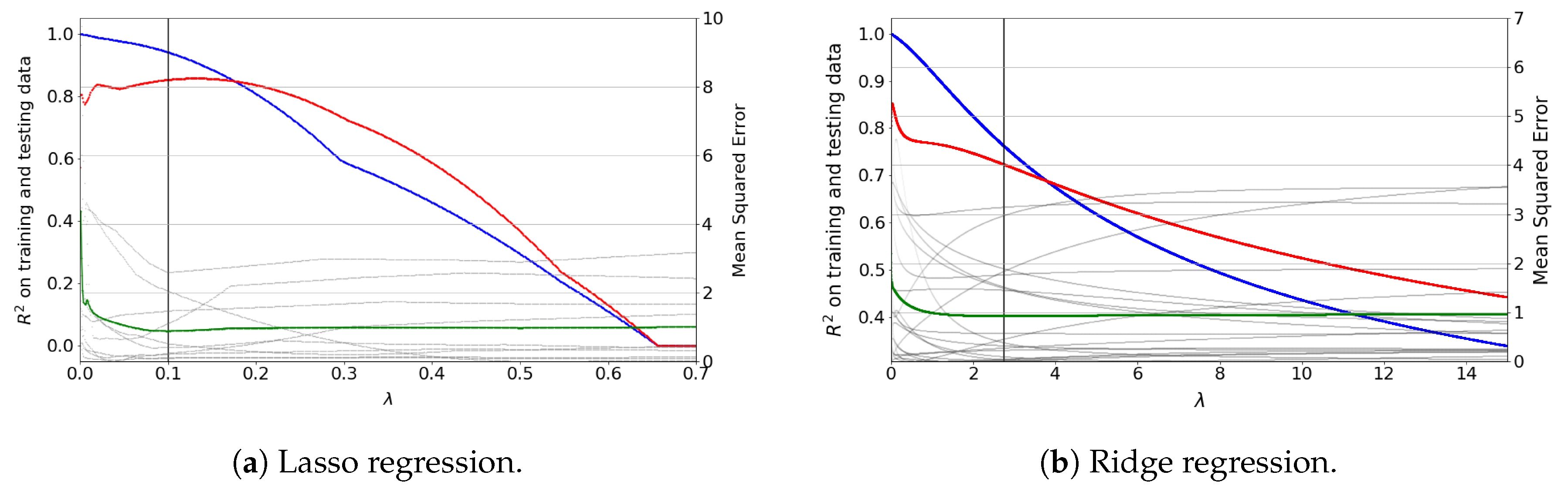
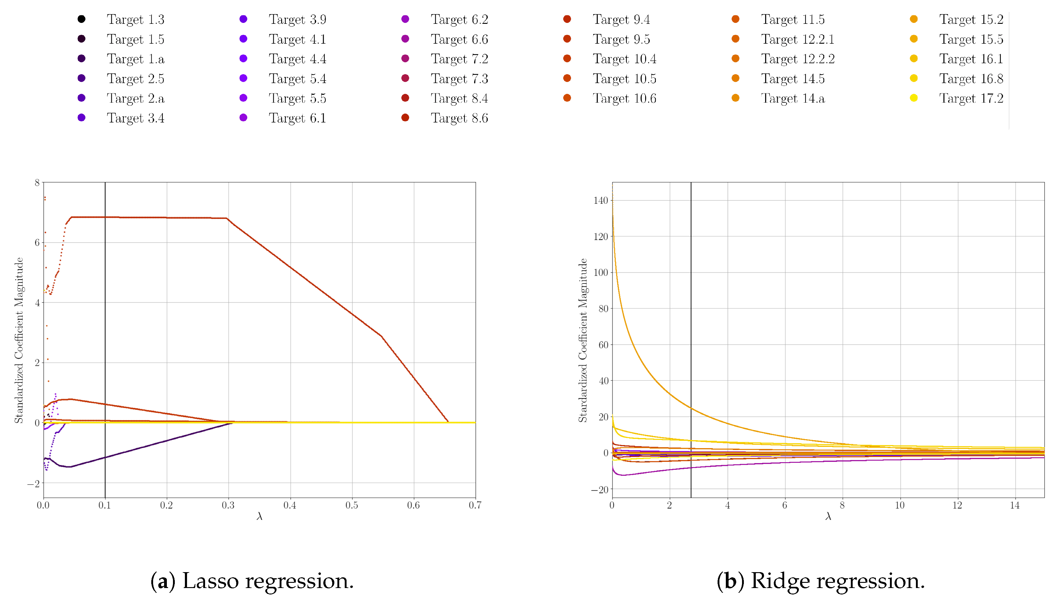
3.3. Regression Analysis

It has been proven that the correlation is a helpful tool when describing the interactions between variables in the past, but no real dependency can be demonstrated. We performed the regression analysis to obtain a mathematical equation between the dependent variable and other targets; so that we could analyse and quantify the influence of enhancing one target on the initial one. After the target selection and timeseries imputation, we achieved a high dimensional dataset (see Appendix A); performing least-squares estimates on it would likely bring over-fitted models with lame predictive behaviour. Thus, irrelevant or partially relevant variables could impact in the model performance negatively, that is why variable selection should be performed using shrinkage methods as stated on Section 2.3. This section delivers the results of performing three shrinkage methods using target 8.6 as dependent variable: lasso, ridge and elastic network regression.

First, lasso regression delivers the minimum MSE of all (0.883). The tuning parameter ($\lambda$) is obtained using 10-fold cross-validation. Figure 4a shows the evolution of the coefficients of determination both for the training (blue line) and the testing (red line) datasets, and the MSE in the secondary axis, as a function of lambda. The dotted grey lines indicate the errors of each fold, so the green line is the average and final considered value. Lambda equals 0.1 delivers the smallest MSE, so the coefficients were calculated using this value. The lasso regression model is formed by nine variables plus the intercept.

Equation (2) captures the true relationship with the independent variables, where the subscript of each X denotes the associated target. The main difference with the correlation coefficient is that Equation (2) is calculated by considering the whole dataset and all the possible interactions, while correlation focuses on a single pair of variables. The lasso regression shrinks 24 of the 33 coefficient estimates to zero, leaving nine predictors plus the intercept to shape the model. They represent the mean response in the dependent variable given a one-unit change in the predictor, and the sign indicates the positive or negative relationship between both variables. For instance, if the response were only dependent on target 4.4, Proportion of youth and adults with information and communication skills went up to 100%, the response variable, Proportion of youth not in education, employment or training would increase in 3%. These coefficients differ from the standardized ones from Figure 5b, since the ones from the equation reflect the real estimate coefficients, reversing the standardizing process.

$$\begin{array}{c}\hfill Y_{8.6}=2.6574+0.1085X_{1.3}+0.0015X_{3.4}-0.0304X_{4.4}+0.1753X_{5.5}-\\ \hfill -0.2279X_{8.4}+0.1807X_{10.5}+0.0384X_{12.2.1}-0.0091X_{14.5}-0.0054X_{15.2}\end{array}$$

(2)

Ridge regression provides slightly higher MSE than lassos: 0.93 over 0.883. The ${\ell }_2$ penalty is added to the original loss function (see Equation (1)). Those tuning parameters $\lambda$ higher than 0.1 are considered as relevant due to the scale of the coefficients as shown in Figure 5b, where the optimal tuning parameter is given by $\lambda$ = 2.738. In this graphic, it can be appreciated that, as the tuning parameter raises, the model becomes more and more biased due to it is stepping away from the un-biased least-squared estimates, in $\lambda$ = 0.

Table 1. Real coefficient magnitudes of the independent variables for ridge regression, including the intercept and considering target 8.6 as dependent variable.

${\mathit{\beta }}_0$	${\mathit{\beta }}_{1.3}$	${\mathit{\beta }}_{1.5}$	${\mathit{\beta }}_{1.\mathit{a}}$	${\mathit{\beta }}_{2.5}$	${\mathit{\beta }}_{2.\mathit{a}}$	${\mathit{\beta }}_{3.4}$
−15.2254	0.12455	0.014690	−0.14922	0.23532	−0.17199	0.0012873
${\mathit{\beta }}_{\mathbf{3}.\mathbf{9}}$	${\mathit{\beta }}_{\mathbf{4}.\mathbf{1}}$	${\mathit{\beta }}_{\mathbf{4}.\mathbf{4}}$	${\mathit{\beta }}_{\mathbf{5}.\mathbf{4}}$	${\mathit{\beta }}_{\mathbf{5}.\mathbf{5}}$	${\mathit{\beta }}_{\mathbf{6}.\mathbf{1}}$	${\mathit{\beta }}_{\mathbf{6}.\mathbf{2}}$
−0.019326	−0.042737	−0.016343	−0.024019	0.23214	0.0056178	0.073088
${\mathit{\beta }}_{\mathbf{6}.\mathbf{6}}$	${\mathit{\beta }}_{\mathbf{7}.\mathbf{2}}$	${\mathit{\beta }}_{\mathbf{7}.\mathbf{3}}$	${\mathit{\beta }}_{\mathbf{8}.\mathbf{4}}$	${\mathit{\beta }}_{\mathbf{9}.\mathbf{4}}$	${\mathit{\beta }}_{\mathbf{9}.\mathbf{5}}$	${\mathit{\beta }}_{\mathbf{10}.\mathbf{4}}$
−0.0041233	0.20411	−0.0011988	−0.43394	0.0038271	0.04316	−0.010594
${\mathit{\beta }}_{\mathbf{10}.\mathbf{5}}$	${\mathit{\beta }}_{\mathbf{10}.\mathbf{6}}$	${\mathit{\beta }}_{\mathbf{11}.\mathbf{5}}$	${\mathit{\beta }}_{\mathbf{12}.\mathbf{2}.\mathbf{1}}$	${\mathit{\beta }}_{\mathbf{12}.\mathbf{2}.\mathbf{2}}$	${\mathit{\beta }}_{\mathbf{14}.\mathbf{5}}$	${\mathit{\beta }}_{\mathbf{14}.\mathbf{a}}$
0.13581	0.0072098	0.014914	0.17754	0.019351	−0.019946	0.021895
${\mathit{\beta }}_{\mathbf{15}.\mathbf{2}}$	${\mathit{\beta }}_{\mathbf{15}.\mathbf{5}}$	${\mathit{\beta }}_{\mathbf{16}.\mathbf{1}}$	${\mathit{\beta }}_{\mathbf{16}.\mathbf{8}}$	${\mathit{\beta }}_{\mathbf{17}.\mathbf{2}}$	${\mathit{\beta }}_{\mathbf{17}.\mathbf{3}}$
−0.0056866	−4.0758 × 10−5	−0.015776	0.0013056	0.0025979	−0.014035

provides the estimate coefficients of the 33 independent variables plus an intercept after considering the target 8.6 as dependent variable. It is notable that some of the less compressed variables in ridge regression match the remaining ones in lasso’s, so both models approximate similar features. These remarkable predictors are: target 1.3 regarding unemployment compensations, target 8.4 relative to the domestic material consumption and target 10.5 respecting non-performing loans were the most significant (see Figure 5a). Apart from these, other predictors are especially considered by ridge regression such as target 2.5 treating the social affairs of local breeds at risk or target 7.2 regarding the renewable energy share consumption. In conclusion, ridge regression might deliver fewer clear results than lasso’s, but it provides a measure of the influence each target has on the response variable, while lasso’s eliminates the superfluous predictors.

Finally, performing elastic network regression on this dataset lead in superimposing lasso’s over ridge’s (see Equation (3)). That is why the resulting coefficient estimates are similar to the ones obtained in lasso regression and their values became akin to lasso’s. This method delivers the highest MSE of the three (0.9553), so the most suitable model to relate the predictors with the dependent variable is the lasso regression, as it delivers the least MSE.

$$\begin{array}{c}\hfill Y_{8.6}=2.6281+0.1052X_{1.3}+0.0015X_{3.4}-0.0326X_{4.4}+0.1671X_{5.5}-\\ \hfill -0.1924X_{8.4}+0.1855X_{10.5}+0.0129X_{12.2.1}-0.0086X_{14.5}-0.0053X_{15.2}\end{array}$$

(3)

4. Conclusions

This research performed a quantitative analysis of synergies and trade-offs between the SDGs of Spain from 2000 to 2019. We assessed the correlation between a handful of indicators representing each SDG instead of considering all the 231 unique indicators. The data relative to these reflected that almost 80% of the significant interactions are classified as synergies or trade-offs. SDG 4 (Quality education), SDG 5 (Gender Equality) and SDG 7 (Affordable and clean energy) are the ones that contain the larger number of positive interactions, more than 60% in all of them. From the correlation analysis, the main ideas prove a positive move toward higher efficiency in energy usage. Spain is running an important energy transition toward greener and renewable sources, but its progress is being slower than other northern countries, as Gales et al. [43] postulated. It seems to work similarly in the health sector. Spain counts as one of the more advanced Public Health systems in Europe [44], and the positive evolution of the sanitation indicators verify this claim (targets 3.9 and 6.2 among others). They are not only fulfilling health-related targets to each other, but also reducing the mortality and benefiting other social indicators.

Each target within this research could be numerically expressed as a regression function of other influential targets. After contrasting with official sources, target 8.6 counted with one of the least geared and most challenging indicators, so a mathematical dependency expression was obtained, and leveraging certain indicators would help to boost its slow-witted tendency. Nonetheless, the results of this study showed that quantifying the indicators regularly is directly related to obtaining a road-map that allows guiding countries towards sustainable development, seizing the available resources and allocating the proper investments in each area. This procedure could offer promising results in the immediate future for the Spanish society. For instance, as the results from regression suggest, target 8.6 is strongly influenced by the the economical situation (target 10.5), consumption habits (target 8.4) and the perception of equal opportunities for leadership (target 5.5) from the Spanish citizens, so improving these aspects positively could leverage desired targets simultaneously since they proved to be interlinked.

We also found inconsistencies in instances that we expected to have the opposite result when assessing the interaction between some indicators. For instances, counterintuitively, we found a negative correlation coefficient amid target 1.a (Ensure significant mobilization of resources [...]) and target 4.1 (ensure that all girls and boys complete free, equitable and quality primary and secondary education [...]). This could be caused by other processes driving both indicators anticlockwise and hence resulting in negative correlation. That is why this research also focused on first quantifying the dependency of each target and then using regression models to project future figures. Furthermore, synergies and trade-offs showed the large share of non-classified interactions for SDG 1 (No poverty) and SDG 10 (Reduced inequalities) compared with the global analysis aforementioned. This suggests that, either the selected targets are not the most appropriate ones, or the Spanish society is not performing the objectives correctly.

Finally, we encourage the policy-makers and people responsible for collecting information about indicators to focus their efforts on launching the mechanisms to guarantee reliable and sufficient data to develop consistent studies regarding sustainability, since other countries reckon on large and extensive analyses. We also urge researchers to deepen the sustainable development outline since important findings can be achieved. The recent research contributes to a strong grounding for the prosperous implementation of the SDGs in Spain. Corroborating with previous research, our findings show that no SDG can individually make a country evolve and comply with the Agenda 2030 but working with the SDGs as a whole can create a virtuous cycle of SDG progress.

References

1. United Nations. Transforming Our World: The 2030 Agenda for Sustainable Development; Division for Sustainable Development Goals: New York, NY, USA, 2015. [Google Scholar]
2. Kroll, C.; Warchold, A.; Pradhan, P. Sustainable Development Goals (SDGs): Are we successful in turning trade-offs into synergies? Palgrave Commun. 2019, 5, 140. [Google Scholar] [CrossRef] [Green Version]
3. Abu-Ghaida, D.; Klasen, S. The Costs of Missing the Millennium Development Goal on Gender Equity. World Dev. 2004, 32, 1075–1107. [Google Scholar] [CrossRef] [Green Version]
4. Fukuda-Parr, S.; Greenstein, J. How Should MDG Implementation be Measured: Faster Progress or Meeting Targets? Working Papers; IPC-IG, International Policy Centre for Inclusive Growth: Brasília, Brazil, 2010. [Google Scholar]
5. Lo Bue, M.C.; Klasen, S. Identifying Synergies and Complementarities Between MDGs: Results from Cluster Analysis. Soc. Indic. Res. 2013, 113, 647–670. [Google Scholar] [CrossRef] [Green Version]
6. OECD. For Good Measure; OECD: Paris, France, 2018. [Google Scholar] [CrossRef]
7. Bennich, T.; Weitz, N.; Carlsen, H. Deciphering the scientific literature on SDG interactions: A review and reading guide. Sci. Total. Environ. 2020, 728, 138405. [Google Scholar] [CrossRef]
8. Allen, C.; Metternicht, G.; Wiedmann, T. Initial progress in implementing the Sustainable Development Goals (SDGs): A review of evidence from countries. Sustain. Sci. 2018, 13, 1453–1467. [Google Scholar] [CrossRef]
9. Griggs, D.J.; Nilsson, M.; Stevance, A.; McCollum, D. A Guide to SDG Interactions: From Science to Implementation; International Council for Science (ICSU): Paris, France, 2017. [Google Scholar]
10. Pradhan, P.; Costa, L.; Rybski, D.; Lucht, W.; Kropp, J.P. A Systematic Study of Sustainable Development Goal (SDG) Interactions. Earth’s Future 2017, 5, 1169–1179. [Google Scholar] [CrossRef] [Green Version]
11. Lusseau, D.; Mancini, F. Income-based variation in Sustainable Development Goal interaction networks. Nat. Sustain. 2019, 2, 242–247. [Google Scholar] [CrossRef] [Green Version]
12. Scharlemann, J.P.W.; Brock, R.C.; Balfour, N.; Brown, C.; Burgess, N.D.; Guth, M.K.; Ingram, D.J.; Lane, R.; Martin, J.G.C.; Wicander, S.; et al. Towards understanding interactions between Sustainable Development Goals: The role of environment—Human linkages. Sustain. Sci. 2020, 15, 1573–1584. [Google Scholar] [CrossRef] [Green Version]
13. Akuraju, V.; Pradhan, P.; Haase, D.; Kropp, J.; Rybski, D. Relating SDG11 indicators and urban scaling—An exploratory study. Sustain. Cities Soc. 2020, 52, 101853. [Google Scholar] [CrossRef]
14. Nerini, F.; Tomei, J.; To, L.; Bisaga, I.; Parikh, P.; Black, M.; Borrion, A.; Spataru, C.; Broto, V.; Anandarajah, G.; et al. Mapping synergies and trade-offs between energy and the Sustainable Development Goals. Nat. Energy 2017, 3, 10–15. [Google Scholar] [CrossRef] [Green Version]
15. Fader, M.; Cranmer, C.; Lawford, R.; Engel-Cox, J. Toward an Understanding of Synergies and Trade-Offs Between Water, Energy, and Food SDG Targets. Front. Environ. Sci. 2018, 6, 112. [Google Scholar] [CrossRef]
16. Scherer, L.; Behrens, P.; de Koning, A.; Heijungs, R.; Sprecher, B.; Tukker, A. Trade-offs between social and environmental Sustainable Development Goals. Environ. Sci. Policy 2018, 90, 65–72. [Google Scholar] [CrossRef]
17. United Nations. Global Sustainable Development Report 2016; United Nations: New York, NY, USA, 2016. [Google Scholar]
18. Nilsson, M.; Chisholm, E.; Griggs, D.; Howden-Chapman, P.; McCollum, D.; Messerli, P.; Neumann, B.; Stevance, A.S.; Visbeck, M.; Stafford-Smith, M. Mapping interactions between the sustainable development goals: Lessons learned and ways forward. Sustain. Sci. 2018, 13, 1489–1503. [Google Scholar] [CrossRef] [PubMed] [Green Version]
19. Coopman, A.; Osborn, D.; Ullah, F.; Auckland, E.; Long, G. Seeing the Whole: Implementing the SDGs in an Integrated and Coherent Way; Stakeholder Forum: London, UK, 2016. [Google Scholar]
20. Saner, R.; Saner, L.; Noah Gollub, Y.; Sidibé, D. Implementing the SDGs by Subnational Governments: Urgent Need to Strengthen Administrative Capacities. PAAP 2017, 20, 23–40. [Google Scholar]
21. Wackernagel, M.; Hanscom, L.; Lin, D. Making the Sustainable Development Goals Consistent with Sustainability. Front. Energy Res. 2017, 5, 18. [Google Scholar] [CrossRef] [Green Version]
22. Mainali, B.; Luukkanen, J.; Silveira, S.; Kaivo-oja, J. Evaluating Synergies and Trade-Offs among Sustainable Development Goals (SDGs): Explorative Analyses of Development Paths in South Asia and Sub-Saharan Africa. Sustainability 2018, 10, 815. [Google Scholar] [CrossRef] [Green Version]
23. Van Soest, H.L.; van Vuuren, D.P.; Hilaire, J.; Minx, J.C.; Harmsen, M.J.H.M.; Krey, V.; Popp, A.; Riahi, K.; Luderer, G. Analysing interactions among Sustainable Development Goals with Integrated Assessment Models. Glob. Transit. 2019, 1, 210–225. [Google Scholar] [CrossRef]
24. Raszkowski, A.; Bartniczak, B. On the Road to Sustainability: Implementation of the 2030 Agenda Sustainable Development Goals (SDG) in Poland. Sustainability 2019, 11, 366. [Google Scholar] [CrossRef] [Green Version]
25. Firoiu, D.; Ionescu, G.H.; Băndoi, A.; Florea, N.M.; Jianu, E. Achieving Sustainable Development Goals (SDG): Implementation of the 2030 Agenda in Romania. Sustainability 2019, 11, 2156. [Google Scholar] [CrossRef] [Green Version]
26. Nilsson, A.E.; Larsen, J.N. Making Regional Sense of Global Sustainable Development Indicators for the Arctic. Sustainability 2020, 12, 1027. [Google Scholar] [CrossRef] [Green Version]
27. Independent Group of Scientists appointed by the Secretary-General. Global Sustainable Development Report. In The Future is Now—Science for Achieving Sustainable Development; United Nations: New York, NY, USA, 2019. [Google Scholar]
28. Weitz, N.; Carlsen, H.; Nilsson, M.; Skånberg, K. Towards systemic and contextual priority setting for implementing the 2030 Agenda. Sustain. Sci. 2018, 13, 531–548. [Google Scholar] [CrossRef] [PubMed] [Green Version]
29. Sachs, J.; Schmidt-Traub, G.; Kroll, C.; Durand-Delacre, D.; Teksoz, K. SDG Index and Dashboards Report 2017; Bertelsmann Stiftung and Sustainable Development Solutions Network (SDSN): New York, NY, USA, 2017. [Google Scholar]
30. Jonathan, D.; Chan, K.S. Time Series Analysis: With Applications in R, 2nd ed.; Springer Texts in Statistics; Springer: Berlin/Heidelberg, Germany, 2008. [Google Scholar]
31. Gallego, I. The Use of Economic, Social and Environmental Indicators as a Measure of Sustainable Development in Spain; Corporate Social Responsibility and Environmental Management: Hoboken, NJ, USA, 2006; pp. 78–96. [Google Scholar] [CrossRef]
32. Boto-Álvarez, A.; García-Fernández, R. Implementation of the 2030 Agenda Sustainable Development Goals in Spain. Sustainability 2020, 12, 2546. [Google Scholar] [CrossRef] [Green Version]
33. Brockwell, P.J.; Davis, R.A. Introduction to Time Series and Forecasting, 3rd ed.; Springer Texts in Statistics; Springer Nature: Berlin/Heidelberg, Germany, 2016. [Google Scholar] [CrossRef]
34. Spearman, C. The proof and measurement of association between two things. Am. J. Psychol. 1904, 15, 72–101. [Google Scholar] [CrossRef]
35. Artusi, R.; Verderio, P.; Marubini, E. Bravais-Pearson and Spearman Correlation Coefficients: Meaning, Test of Hypothesis and Confidence Interval. Int. J. Biol. Markers 2002, 17, 148–151. [Google Scholar] [CrossRef] [PubMed]
36. Hauke, J.; Kossowski, T. Comparison of Values of Pearson’s and Spearman’s Correlation Coefficients on the Same Sets of Data. Quaest. Geogr. 2011, 30, 87–93. [Google Scholar] [CrossRef] [Green Version]
37. Sesnie, S.; Tellman, B.; Wrathall, D.; McSweeney, K.; Nielsen, E.; Benessaiah, K.; Wang, O.; Reymondin, L. A spatio-temporal analysis of forest loss related to cocaine trafficking in Central America. Environ. Res. Lett. 2017, 12, 1–19. [Google Scholar] [CrossRef] [Green Version]
38. Sidney, J.A.; Jones, A.; Coberley, C.; Pope, J.E.; Wells, A. The well-being valuation model: A method for monetizing the nonmarket good of individual well-being. Health Serv. Outcomes Res. Methodol. 2017, 17, 84–100. [Google Scholar] [CrossRef] [Green Version]
39. James, G.; Witten, D.; Hastie, T.; Tibshirani, R. (Eds.) An Introduction to Statistical Learning: With Applications in R; Springer Texts in Statistics; Springer: Berlin/Heidelberg, Germany, 2013. [Google Scholar]
40. Karl Härdle, W.; Simar, L. Applied Multivariate Statistical Analysis, 4th ed.; Springer: Berlin/Heidelberg, Germany, 2014. [Google Scholar] [CrossRef]
41. Montgomery, D.C.; Peck, E.A.; Vining, G.G. Introduction to Linear Regression Analysis, 5th ed.; Wiley Series in Probability and Statistics 821; John Wiley & Sons, Inc.: Hoboken, NJ, USA, 2012. [Google Scholar]
42. Frank, E.; Harrell, J.R. Regression Modeling Strategies: With Applications to Linear Models, Logistic and Ordinal Regression, and Survival Analysis, 2nd ed.; Springer Series in Statistics; Springer: Berlin/Heidelberg, Germany, 2015. [Google Scholar] [CrossRef]
43. Gales, B.; Kander, A.; Malanima, P.; Rubio, M. North versus South: Energy transition and energy intensity in Europe over 200 years. Eur. Rev. Econ. Hist. 2007, 11, 219–253. [Google Scholar] [CrossRef] [Green Version]
44. World Health Organization. The World Health Report: Health System: Improving Performance; World Health Organization: Geneva, Switzerland, 2000. [Google Scholar]
Figure 1. Main stages of statistical analyses performed.
Sustainability 12 10506 g001
Figure 2. Correlation matrix in pairs using the Spearman’s coefficient, significant values only. The colour scale represented by blue and red shines. Red scale stands for the negative correlation coefficients and the blue scale does the same for positive ones.
Sustainability 12 10506 g002
Figure 3. Observed synergies (green bars), trade-offs (orange bars) and non-classified interactions (blue bars) between targets at the goal level. Classification stated on Section 2.2. Share in (%).
Sustainability 12 10506 g003
Figure 4. R 2 values for training (blue) and testing (red) data as a function of λ . The green line represents the average MSE obtained by cross-validation. The vertical black line is the optimal tuning parameter λ for each regression method.
Sustainability 12 10506 g004
Figure 5. Standardized coefficients of the independent variables for target 8.6 as a function of λ .
Sustainability 12 10506 g005