Connection of Solar Activities and Forest Fires in 2018: Events in the USA (California), Portugal and Greece

Abstract

The impact of solar activity on environmental processes is difficult to understand and complex for empirical modeling. This study aimed to establish forecast models of the meteorological conditions in the forest fire areas based on the solar activity parameters applying the neural networks approach. During July and August 2018, severe forest fires simultaneously occurred in the State of California (USA), Portugal, and Greece. Air temperature and humidity data together with solar parameters (integral flux of solar protons, differential electron flux and proton flux, solar wind plasma parameters, and solar radio flux at 10.7 cm data) were used in long short-term memory (LSTM) recurrent neural network ensembles. It is found that solar activity mostly affects the humidity for two stations in California and Portugal (an increase in the integral flux of solar protons of > 30 MeV by 10% increases the humidity by 3.25%, 1.65%, and 1.57%, respectively). Furthermore, an increase in air temperature of 10% increases the humidity by 2.55%, 2.01%, and 0.26%, respectively. It is shown that temperature is less sensitive to changes in solar parameters but depends on previous conditions (previous increase of 10% increases the current temperature by 0.75%, 0.34%, and 0.33%, respectively). Humidity in Greece is mostly impacted by solar flux F10.7 cm and previous values of humidity. An increase in these factors by 10% will lead to a decrease in the humidity of 3.89% or an increase of 1.31%, while air temperature mostly depends on ion temperature. If this factor increases by 10%, it will lead to air temperature rising by 0.42%.

1. Introduction

The energy input from the Sun is a driving factor in Earth’s climate system. It is very difficult to estimate how the changes in solar activities can affect the dynamics of many environmental processes. The previous studies found statistical connections between the occurrences of forest fires in various regions worldwide and the emissions from the Sun [1,2,3,4,5]. The main hypothesis is that the emissions of high-speed and high-energy particles from coronary holes and/or energetic regions with geo-effective positions precede the fires that happen at the same time but in geographically different regions [6]. For proving these statements, various mathematical and statistical models, mainly from the data mining field, were used to achieve the nonlinear behavior of meteorological and solar activity parameters. The present study looks for new evidence in the cases of forest fires recorded in July and August 2018 and processes of the Sun.

During 2018, severe forest fires were reported in many parts of the world [7,8]. The 2018 California fire season was the worst in the previous 15 years (8054 fires, total burned area was 737,803.9 ha) [9]. The greatest damage and the highest number of human casualties were recorded from mid-July to mid-August. The Mendocino Complex Fire broke out on 27 July, and it was the greatest wildfire in the history of California. The total burned area was 185,800.5 ha, and the greatest damage was recorded in August [10]. In Portugal, the most serious problems with wildfires were recorded in August, and the greatest wildfire was from 3 to 10 August in Faro District (Algarve), which burned 27,764 ha. In the fires in Attica, Greece, 102 human casualties were recorded in the period 23–26 July [11].

The aim of this paper is to find and investigate dependencies between the aforementioned fires and solar activity using long short-term memory (LSTM) recurrent neural network ensembles. As a result of establishing the function relation between weather and solar parameters, forecast models will be produced.

2. Materials and Methods

The data on fires in California were provided by the California Department of Forestry and Fire Protection (CAL FIRE) [10] and the National Interagency Coordination Center (NICC) [12]. For Portugal and Greece fires, the source was the European Commission’s Science and Knowledge Service [11]. Meteorological data and solar activity data were used in the calculations. The weather data included air temperature and humidity. For California, the data from Redding Municipal Airport (40°30′32″ N 122°17′36″ W) [13], Del Norte County Airport (41°46′49″ N 124°14′12″ W) [14], and Sacramento International Airport (38°41′44″ N 121°35′27″ W) [15] weather stations were used (in the further text referred to as California 1, California 2, and California 3, respectively). The data from Faro Airport Station, Portugal weather station (37°00′52″ N 007°57′57″ W) [16], and Athens International Airport, Greece weather station (37°56′11″ N 23°56′50″ E) [17], were also used in the research (in the further text referred to as Portugal and Greece, respectively). All aforementioned stations were selected because of their proximity to the area affected by fires. The data cover the period 16 July–13 August 2018 (16 July–16 August 2018, for Portugal), as presented in

Table 1. Data observational periods and modeled forecast periods for the three different study areas.

Study Area	Observational Period	Forecast Period
California	16 July–13 August	3–11 August
Portugal	16 July–16 August	3–16 August
Greece	16 July–13 August	17–26 July

.

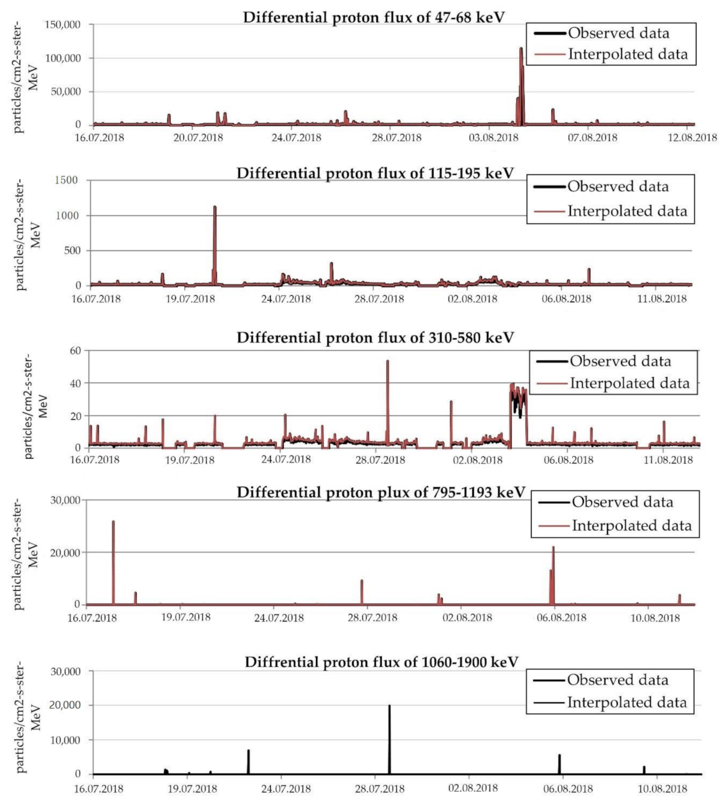
The main source for proton and electron flux was the Space Weather Prediction Center [18]. The data included the 5-min averaged integral flux of solar protons (>10 and >30 MeV) and the 5-min averaged differential electron and proton flux. The data on differential electron flux included 38–53 and 175–315 keV. The data on differential proton flux included 47–68, 115–195, 310–580, 795–1193, and 1060–1900 keV. The source for the 1-min averaged bulk parameters of solar wind plasma was also the Space Weather Prediction Center [19]. The data included proton density (p/cc), bulk speed (km/s), and ion temperature (K). The source of data on solar flux F10.7 cm (2800 MHz) was Space Weather Canada [20]. The F10.7 cm solar radio flux (or just F10.7) is, along with the sunspot number, one of the most widely used indices of solar activity [21]. The data on proton and electron flux and solar flux F10.7 cm cover the period 16 July–16 August 2018 [22].

The large number of asynchronous data coming from different sources [23,24,25] and the lack of a physical model of the process suggest a methodology associated with a category of big data. The used methodology is based on the data mining approach. The assumption about the time delay between the solar activity and atmospheric processes suggests that recurrent neural networks should be used in the calculations. The best results for such data are obtained through LSTM ensembles [20]. The analysis was conducted through the following steps:

• Preliminary analysis of incoming and outgoing data;
• Import and integration of data into a sparse matrix;
• Data retrieval to the equal time range;
• Filling missing data;
• Reducing the number of input factors;
• Creation of normalized training and test samples;
• Creation and fitting of LSTM recurrent neural network ensembles;
• Check for adequacy and analyze the sensitivity of the model’s ensemble.

2.1. Preliminary Analysis of Incoming and Outgoing Data

The parameters of the solar activity were observed for the period from 16 July to 16 August 2018. Within this period, data were divided into training and forecast (test) sets (Table 1). In the case of Portugal, the training set is from 16 July to 2 August and the forecast set is 3–16 August. For California and Greece, the training sets consist of two data blocks located within observational periods indicated in Table 1 (note that in the case of California, one of the tests is closer to the end, and for Greece, the forecast data are at the beginning of the observation period).

Different measurement (sampling) intervals for modeled input parameters mean different time scales of both input and target data sets. In the case of solar parameters, the data are presented by averaged values for a certain time interval (1 and 5 min) or measurements are performed several times per day (for F10.7 cm, the measuring times are 17:00, 20:00, and 23:00). The information about time sampling is given in

Table 2. Time sampling of input and output parameters and corresponding data frames (DFs).

Data Frame (DF)	Input and Target Factors	Time Sampling
1	Integral flux of high-energy solar protons of Field 1: >10 MeV, Field 2: >30 MeV	5 min
2	Differential electron flux and proton flux of Field 1: 38–53 keV, Field 2: 175–315 keV, Field 3: 47–68 keV, Field4: 115–195 keV, Field 5: 310–580 keV, Field 6: 795–1193 keV, Field 7: 1060–1900 keV	5 min
3	Field 1: proton density, Field 2: bulk speed, Field 3: ion temperature	1 min
4	Field 1: F10.7 cm	3 per day (17:00, 20:00, and 23:00)
5	Field 1: air temperature, Field 2: humidity	15 min–1 h (California) 30 min (Portugal and Greece)

. According to their sources, all the data were grouped in corresponding data frames (DFs). A large number of missing values in time series within frames 1–4 was found, and interpolation was applied. All time series were adjusted to UTC in order to overcome the problem of the observational records being in different time zones.

The plots of time series are presented in Appendix A (Figure A1, Figure A2, Figure A3, Figure A4, Figure A5, Figure A6, Figure A7, Figure A8, Figure A9 and Figure A10).

2.2. Import and Integrate Data into a Sparse Matrix

Unlike time series, the DF consists of tuples of values. Each tuple corresponds to the measurement date/time (index field):

(1)

where f is the frame number from Table 2 and $Fiel{d}_{fi}$ is the i-input (target) field of frame f.

According to Table 2, there are four DFs of input fields and five separate DFs for each station (California 1, California 2, California 3, Portugal, and Greece). The next step was to merge all DF_f accordingly to the index fields into one DF. As a result, 5 separate DFs were receiving for each station, respectively:

$$D{F}^s=D{F}_1\cup D{F}_2\cup D{F}_3\cup D{F}_4\cup D{F}_5^s$$

(2)

where s is the station index.

The obtained $D{F}^s$ contains a set of all possible values of index fields from all $D{F}_f$. The missing fields are filled with blank cells. As the result, the tuple values of the fields ${\mathrm{DF}}^s$ are presented as a sparse matrix and the index field had an uneven discretization in time.

2.3. Data Retrieval to the Equal Time Range

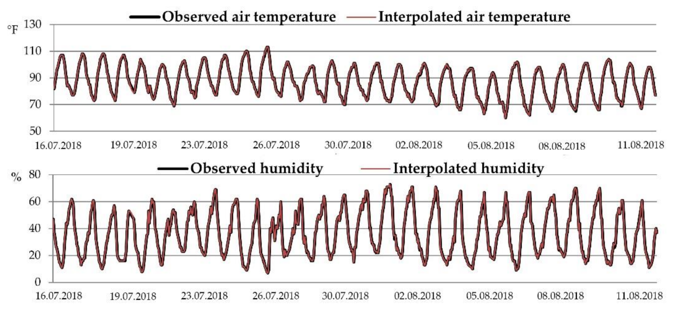
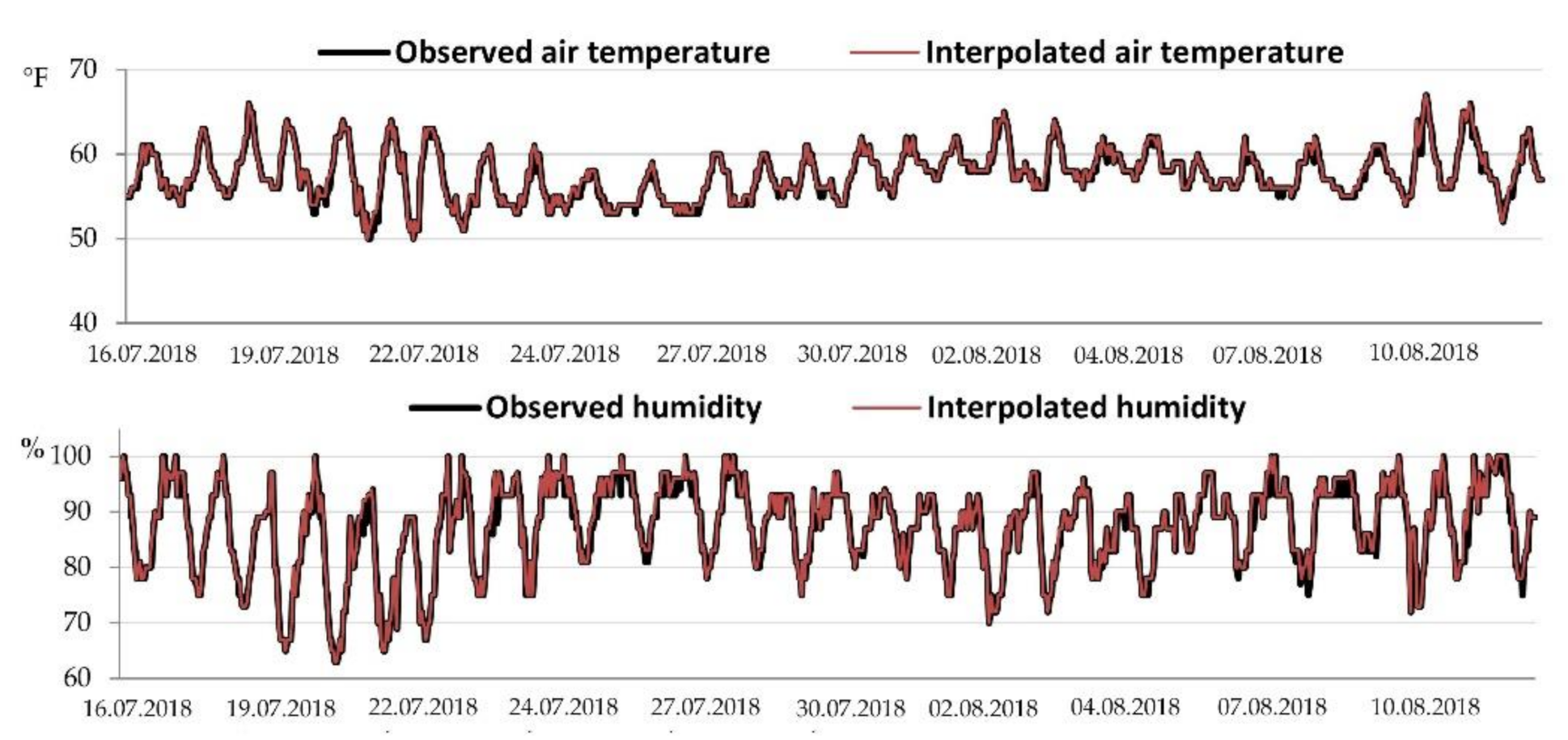
The transformation of $D{F}^s$ by entering the equal sampling time step for all the fields is necessary in order to obtain a training sample suitable for model learning. The target fields consist of the data with a sampling step from 15 min to 1 h, while for input fields, the sampling step is significantly smaller (Table 2). Increasing the sampling step to one hour will lead to losing information about fluctuations in the input fields and a significant reduction in the training set. Reducing the sampling step to 30 min will require interpolation of data for stations in California 1 and California 3. It can lead to the possible accumulation of false data. However, the dynamics of data for these stations are sufficiently smooth (Figure A6 and Figure A8), which allows us to carry out additional interpolation for decreasing sampling without a loss of accuracy. Therefore, a 30-min range was selected as a sampling time step.

The data that fell within the 30 min range were joined by operation Max for increasing the sampling rate to the abovementioned range in the case of frames 1–3 input fields (Table 2):

$$D{F}^s\underset{\mathit{max}\left(∆Key=t\right)}{\to }D{F}^{s, t}$$

(3)

where $t$ = 30 min.

The equal sampling time step enables us to take into account solar flares that were observed in these ranges (Figure A1, Figure A2, Figure A3 and Figure A4) and to eliminate abnormal negative vibrations. As a result, the total number of DF rows decreased from about 47,000 to 1120 (California and Greece) and 1310 (Portugal).

2.4. Filling Missing Data

It was possible to eliminate the overwhelming number of the missing data as a result of previous data transformation. Spline cubic interpolation was used for each field to eliminate the problem with missing data at the beginning and end of time series and the missing data inside the fields California 1 and California 3 and F10.7 cm [26]. A four-point rolling window was used to reduce white noise [27]. The interpolation was conducted as

$$D{F}^{s,t}\underset{\mathrm{s}plin{e}^3, rolling window}{\to }D{F}^{s, t,inp}$$

(4)

where $t$ = 30 min.

The interpolation results are shown in Figure A1, Figure A2, Figure A3, Figure A4, Figure A5, Figure A6, Figure A7, Figure A8, Figure A9 and Figure A10. The max-cubic-spline interpolation allowed cutting off the minima and highlighting the biggest outbreaks of solar activity parameters (Figure A1, Figure A2, Figure A3 and Figure A4). This approach enabled us to determine the intermediate values for the time series F10.7 cm, California 1, and California 3 (Figure A5, Figure A6 and Figure A8). The dynamics of the change in these indicators were quite smooth, so spline interpolation showed good results. As shown in Figure A6 and Figure A8, data interpolation for California 1 and California 3 completely repeats the original time series, giving the right to assert that there is no false data in the interpolation.

2.5. Reducing the Number of Input Factors

Autocorrelation analysis was performed between all the fields of $D{F}^{s,t,inp}$ to reduce the number of input parameters. The studied periods for the stations in California and Greece coincide (Table 1), but in the case of Portugal, the period is slightly longer, which makes the results of the autocorrelation somewhat different. The resulting matrices of all the possible pairwise coefficients of correlation between all the input and output fields are presented in

Table 3. Results of autocorrelation analysis for California and Greece.

and

Table 4. Results of autocorrelation analysis for Portugal.

. Each of the cells is a symmetric matrix and consists of correlation coefficients between two separate factors.

All the correlation coefficients are essentially small except in the case of the integral flux of high-energy solar protons of > 10 and > 30 MeV (with a value of 0.93). In addition, the high negative coefficients are between the output fields of air temperature and humidity. The results suggest that one of the input fields can be neglected. The field of the integral flux of high-energy solar protons of > 30 MeV was selected and used in further calculations. As a result, the $D{F}^{s,res}$ was obtained by extracting a field $>10 \mathrm{MeV}$ from $D{F}^{s,t,inp}$:

$$D{F}^{s,t}\underset{\mathrm{s}plin{e}^3, rolling window}{\to }D{F}^{s, t,inp}$$

(5)

The resulting DF contains 12 input fields and 2 outputs.

2.6. Creation of Normalized Training and Test Samples

Low values of the correlation coefficients can imply the presence of nonlinear functional dependencies. To prove this, it is necessary to normalize all the incoming and outgoing data ($D{F}^{s,res}\underset{}{\to }{\widetilde{DF}}^{s,res}$). This will reduce the rounding error when fitting neural networks. The next step involves consideration of the effects of input factors on target factors with a certain delay in time t_L (L—the time lag). In addition, target factors represent a complex system that depends on other factors that are not taken into account in this step. It is necessary to add the value of the target fields in the previous interval of time to the input factors in order to take into account their lag influence (t_L). The previous studies [28] indicated the L takes up to 4 days = 24 × 4 h. Taking into account the sampling rate of 30 min (twice per hour), this will increase the input factors from 14 (12 input + 2 output) to $N=14\times 4\times 24\times 2=2688$, making it impossible to solve the problem with classical neural networks and other regression models. On the other hand, it is possible to use either a complete overview of all the possible models with all the possible combinations and the number of input factors [29] or to use the recursive neural network LSTM that has been developed specifically for this type of task [30]. A feature of this recurrent neural network is that its inputs are not individual values at a particular point in time, but rather time series of historical values of input values in the form of vectors, the length of which is equal to the value of the investigated lag. In the fitting process, LSTM treats the vector’s historical data as a prior experience and returns the modified input values via recurrent connections to the input. Thus, it is possible to analyze the impact of values at previous times. The peculiarity is that the size of the input vectors does not play a big role. Therefore, we did not investigate dependencies results on lag size. We used the maximum possible value for 4 days.

When using this type of neural network, each of the received ${\widetilde{DF}}^{s,res}$ must first be transformed into a shape:

(6)

where t is the date and time of the key field, $\widetilde{In}$ and $\tilde{T}$ are normalized input and output fields, respectively, and $L= 4\times 24\times 2=192$ is the maximum value of lag.

The next step is to split ${\widetilde{DF}}_{LSTM}^{s,res}$ into input and output data. The last three fields of the tuple $Data$ were selected as the target, the other was the input:

(7)

$$\begin{array}{ll}{\widetilde{DF}}_{LSTM, in}^{s,res}=(Key& =t: Dat{a}_{in}^s=\\ & <{\widetilde{In}}_1\left(t-1\right),\dots ,{\widetilde{In}}_{12}\left(t-1\right),{\tilde{T}}_1\left(t-1\right),{\tilde{T}}_2\left(t-1\right),\dots ,{\widetilde{In}}_1\left(t-t_L\right),\dots ,{\widetilde{In}}_{12}(t\\ & -t_L),{\tilde{T}}_1\left(t-t_L\right),{\tilde{T}}_2{\left(t-t_L\right)}_{}>)\end{array}$$

(8)

Then, the tuple of the input field values was transformed into a three-dimensional form:

$${\widetilde{DF}}_{LSTM, in}^{s,3D}=(Key=t: Dat{a}_{in}^{s, 3D}={\left\{d_{t,l,f}\right\}}_{t=\overline{1,{\mathrm{r}}_s}, l=\overline{1,192},f=\overline{1,15}}>)$$

(9)

where $d$ is the input field of tuple $Dat{a}_{in}^{s,}$, and indexes, t is time (number of rows), l is lag, f is input fields, and $r_s$ is the number of rows of ${\widetilde{DF}}_{LSTM}^{s,res}$ for the corresponding station s.

In other words, the input of the neural network must be submitted to the two-dimensional array. Each column of the array represents a time series of input and target factors for the previous time lag t_L. The target consists of two outputs (air temperature and humidity).

The data for each training set for the individual station s (${\widetilde{DF}}_{LSTM, in}^{s,3D}$ and ${\widetilde{DF}}_{LSTM, tar}^{s,res}$) were divided into training and test sets according to the dates specified in Table 1.

2.7. Creation and Fitting of LSTM Recurrent Neural Network Ensembles

As noted above, a recurrent neural network LSTM was selected as the working model. It allows the simulation of the behavior of a system that depends on time. This is realized by reverse transmission of the output signal of the neural network at the time t − 1 back to the input of one of the network layers at time t.

As the test calculations show, the best results were obtained for the LSTM of the following configuration: the number of inputs is 12, the number of outputs is 2, the number of neurons is 50, the batch size of the training set is 10% (learning was carried out by batch of the data of the training set), the training epoch was determined dynamically in the fitting process with the aim to avoid overtraining, accuracy criterion—mean square error, and learning method—Adam [31]. The structure of the neural network was obtained using the TensorBoard library called TensorFlow.

The dynamics of the change in the mean square error of the test and training sets during the fitting of one of the neural networks are presented in Figure 1. As can be seen on the plot, there are several peaks of increased errors that can be explained by the transition to the next batch of training. To determine the required number of epochs and the number of neurons, the dynamics of the change of the mean square error during the training period were investigated. The training stopped when the test set error on the plot began to grow steadily over the course of 10 periods of study. As it is shown, the neural network adapted rather quickly to the training set and for a long time for the test set. This indicates the need for deep learning. Moreover, the error of the test and training sets varies greatly among them, indicating the presence of sufficiently complex functional dependencies.

2.8. Check for Adequacy and Analyze the Sensitivity of the Models Ensemble

The obtained models give us an opportunity to calculate the sensitivity of the output fields from the influence on the inputs. To do this, the value of the ensemble of models is calculated for each record j in ${\widetilde{DF}}_{LSTM, in}^{s,3D}$, where M is the number of records in the DF. In the next step, all values of the time series of factors i = 1–15 in (${\widetilde{DF}}_{LSTM, in}^{s,3D}$ are incremented gradually by 10%.

Then, the initial values are calculated: . The next step is to calculate the relative change matrix for each entry:

$$Se={\left\{s{e}_j^i\right\}}_{i=\overline{1,15},j=\overline{1,M}}={\left\{\frac{Dat{a}_{tar,i}^{s,En}-Dat{a}_{tar}^{s,En}}{Dat{a}_{tar}^{s,En}}\right\}}_{i=\overline{1,15}}$$

(10)

where i is the index of the input parameter and j is the row index.

The vector of the averaged effect of each factor on the whole row is calculated after $Dat{a}_{tar}^{s,En}$ has been calculated:

$$\overline{Se}={\displaystyle \sum }_{j=1}^{M}s{e}_j^i$$

(11)

3. Results and Discussion

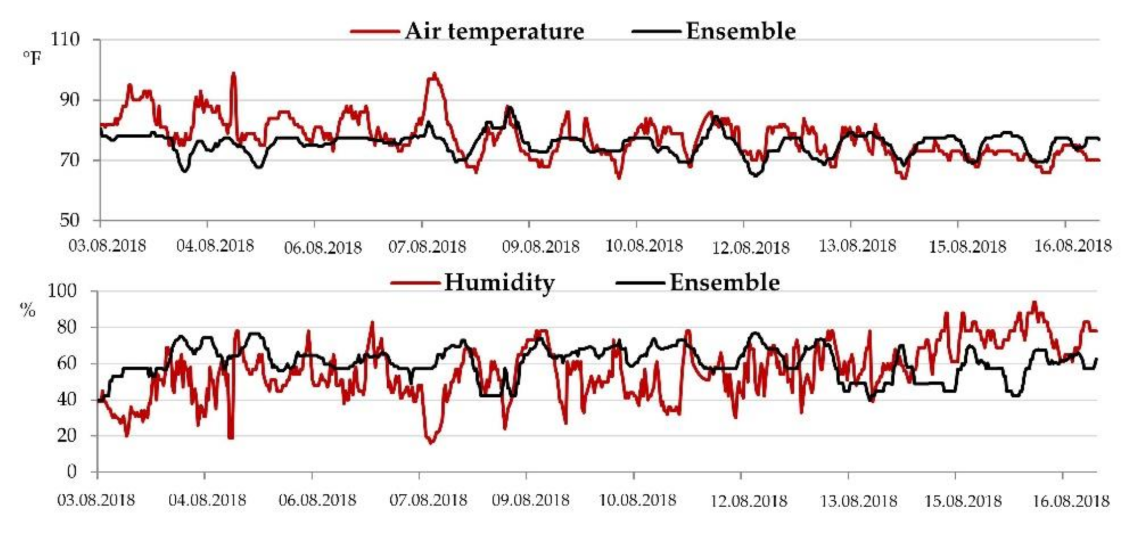
The forecast results for nine neural networks for the training set are presented in Figure 2, Figure 3, Figure 4, Figure 5 and Figure 6. As can be seen from the figures, all the neural networks’ forecasts showed good agreement with the training sets. However, there are strong fluctuations in the test sets. In particular, the weakest forecasts were obtained in the cases of Greece and California 2. The best prediction results are observed in the cases of stations California 1 and California 3. It is also clearly seen from the graphs that, in the cases of California 2, Greece, and Portugal, the problem of stability remains as the open question, and hence the accuracy and adequacy of different LSTM models. To solve this, LSTM ensembles based on gradient boosting (GB) for regression were used. The GB builds an additive model in a forward stage-wise fashion, and it allows for the optimization of arbitrary differentiable loss functions. In each stage, a regression tree is fitted on the negative gradient of the given loss function [32,33,34].

The mean square error was chosen as the optimization criterion, the number of boosting stages to perform was equal to 100, the learning rate = 0.1, and the maximum depth of the individual regression estimators = 1. The following results were obtained on the test data (Figure 7, Figure 8, Figure 9, Figure 10 and Figure 11). This plot shows the forecast results with a comparison of real data.

Visually comparing the two curves on the figures, we can conclude the level of the forecast accuracy. As can be seen from the figures, the best results of the ensemble prediction are in the cases of California 1 and California 3. For the quantitative estimation of the accuracy of the ensemble of models, it is convenient to conduct a correlation analysis between the time series of real data and separate LSTM models plus the ensemble (

Table 5. Pearson correlation coefficients of the obtained models.

	LSTM1	LSTM2	LSTM3	LSTM4	LSTM5	LSTM6	LSTM7	LSTM8	LSTM9	Ensemble
California 1
T	0.90	0.93	0.90	0.89	0.93	0.86	0.91	0.95	0.86	0.91
H	0.87	0.93	0.92	0.89	0.93	0.89	0.92	0.91	0.89	0.92
California 2
T	0.29	0.37	0.37	0.29	0.31	0.17	0.36	0.36	0.24	0.29
H	0.27	0.38	0.49	0.28	0.27	0.24	0.39	0.39	0.16	0.33
California 3
T	0.93	0.90	0.91	0.92	0.94	0.92	0.93	0.93	0.92	0.93
H	0.90	0.90	0.90	0.90	0.90	0.90	0.90	0.90	0.91	0.91
Portugal
T	0.44	0.35	0.42	0.48	0.57	0.40	0.39	0.42	0.45	0.44
H	0.04	0.00	0.06	0.19	0.10	0.09	0.07	0.17	−0.01	0.04
Greece
T	0.71	0.62	0.70	0.70	0.81	0.58	0.70	0.59	0.67	0.75
H	0.63	0.49	0.55	0.59	0.69	0.63	0.50	0.56	0.52	0.60

).

Each cell of the table contains correlation coefficients between real data and forecasts using separate models. The last column (far right) contains the correlation coefficient of the ensemble. According to calculated correlation coefficients, the most accurate models were obtained for California 1 and 3 and for Greece. The forecast data for Portugal and California 2 are totally uncorrelated with the actual data. This may indicate that the models obtained for these stations are unsuitable. Therefore, it is necessary to take into account completely different factors for constructing adequate models for these stations. The results of the sensitivity of the output fields from the influence on inputs are presented in

Table 6. Sensitivity analysis of air temperature (T) and humidity from solar activity factors (in %).

Input Factor	Solar Proton Flux of > 30 MeV	Differential Electron Flux of 38–53 keV	Differential Electron Flux of 175–315 keV	Differential Proton Flux of 47–68 keV	Differential Proton Flux of 115–195 keV	Differential Proton Flux of 310–580 keV	Differential Proton Flux of 795–1193 keV	Differential Proton Flux of 1060–1900 keV	Proton Density	Bulk Speed	Ion Temperature	F10.7 cm	T	H
California 1
T	0.59	0	0	−0.01	0.01	0.12	0.01	0	−0.06	0.09	0	0.25	0.75	−0.03
H	3.25	0	0	0.11	0.09	0.31	−0.02	−0.01	−0.34	−0.23	0.03	0.96	2.55	−1.10
California 2
T	−0.06	0	0	0.03	0.03	0.02	0.01	0	0	−0.12	0	−0.03	0.27	0.33
H	0.07	0	0	−0.07	−0.02	0.31	0.13	−0.07	0	0.18	0	−0.46	−0.21	0.10
California 3
T	0.38	0	0	0	0.08	0.09	0	0	−0.02	0.06	0	0.48	0.34	−0.01
H	1.65	0	0.01	0.08	0.01	0.22	−0.04	0.01	−0.07	0.14	0.05	1.26	2.01	0.85
Portugal
T	0.35	0	0	0.02	0.04	0.08	−0.01	0	−0.01	−0.10	−0.03	−0.14	0.33	0.06
H	1.57	0	0	0.03	0.02	−0.53	0	−0.01	0	0.32	0.10	0.71	0.26	1.62
Greece
T	0.30	0	0	0.01	0.02	−0.01	0	−0.05	−0.23	0	0.42	−0.08	0.01	0.37
H	0.04	0	0.01	−0.03	−0.08	0.10	0.06	0.07	0.01	1.06	0.15	−3.89	0.02	1.31

.

The cells of the table show the percent of which the temperature or humidity will change by with each factor changing by 10% of its average value. All other factors are fixed on averages values. The results of the sensitivity analysis suggest that solar activity mostly affects the humidity for stations California 1, California 3, and Portugal. It is shown that an increase in the factor integral flux of high-energy solar protons of > 30 MeV by 10% increases the humidity by 3.25%, 1.65%, and 1.57% at stations California 1, California 3, and Portugal, respectively. Moreover, an increase in temperature by 10% increases the humidity by 2.55%, 2.01%, and 0.26% at these stations, respectively. The temperature is less sensitive to the changes in factors, especially in the case of Portugal. The growth in the same factor by 10% increases the air temperature by 0.59%, 0.38%, and 0.35% at California 1, California 3, and Portugal, respectively. Additionally, it was found that temperature depends on its previous conditions, i.e., previous increase by 10% increases the current temperature by 0.75%, 0.34%, and 0.33%, respectively. It is also visible that the humidity depends on the changes in temperature, but the reverse effect is not observed. For Greece, we obtained another result. The humidity is mostly affected by F10.7 and previous values of humidity. An increase in these factors of 10% will lead to a decrease in the humidity of 3.89% and 1.31%, respectively. If this factor increases by 10%, it will lead to an increase in the temperature of 0.42%.

Even if the possible role of pyromaniacs (as well as any other potential explanation regarding the direct or indirect role of man) is accepted for the occurrence of fires in specific locations, it remains unclear how there is a selective ignition of vegetation in remote places on the same day [35]. In recent years, there were several papers where forest fires were brought into connection with solar activity [1]. In these studies, findings highlighted a hypothesis that the charged particles of the solar wind in certain conditions reach the surface of Earth, where they can cause fires in vegetation. Many of the mentioned papers refer to the individual cases of fires in the periods not longer than a month. With this in mind, the results put forward the “heliocentric hypothesis” that those forest fires without established causes were caused by a burning plant mass under the action of charged particles that come to us from the Sun. The authors suggested that the occurrence of the fire should be preceded by and correlated with a sudden influx of the mentioned particles toward our planet. A theoretical model, according to which the charged particles penetrate the ground through the geomagnetic anomaly and, after scattering on the ground, could cause burning of biomass, for the first time, to our knowledge, was presented by Gomes and Radovanović [6]. The report by Baldwin and Dunkerton [36] showed that stratospheric mean flow variations induce circulations that penetrate into the lower troposphere. To investigate these results more in detail, Boberg and Lundstedt [37] used the geopotential height (GPH) data on 16 pressure levels covering both hemispheres to see if the proposed correlation exists in the terrestrial stratosphere and troposphere. The results show a high statistical connection between solar wind electric field (E) and geopotential height (E-GPH statistical connection), extending from the lower stratosphere down to the surface. “However, the physical mechanism of solar activity effects on weather phenomena remains unclear. It is suggested that a significant part in the transfer of the solar variability to the lower atmosphere may be played by charged particles of solar and galactic origin, mainly protons, with energies from ~100 MeV to several GeV“ [38]. As Tinsley and Yu [39] stated, “there has not been any decisive result which would discern how many of the monitored decade variations were formed because of the entry of the flux of particles, comparing to the total or spectral changes of radiation. However, there is not such ambiguity concerning the correlation of the atmospheric dynamics with particle flows on the weather scale day after day.”

In addition, the role of lightning as the initiator of forest fires is often confusing, mainly because it is accompanied by the appearance of rain. As Hall points out from 1990 to 1998, over 17,000 naturally ignited wildfires were observed in Arizona and New Mexico on US federal land during the fire season of April through October [40]. Lightning strikes associated with these fires accounted for less than 0.35% of all recorded cloud-to-ground lightning strikes.

Viewing from the presented perspective, Lynch et al. [41] stressed the importance of the domain of the key question, but obviously without a clear vision of how to further develop the measures of prevention: “Our results therefore support other recent studies demonstrating that warmer/drier climatic conditions do not necessarily induce greater fire importance. These results contradict the current understanding of modern fire–climate relationships. It is also inconsistent with model predictions that a drier and warmer climate, as a result of glasshouse warming, will lead to increased fire activity in boreal systems”. Gorte and Bracmort’s [42] study was more categorical, and the authors stated that “research information on causative factors and on the complex circumstances surrounding wildfire is limited. The value of wildfires as case studies for building predictive models is confined, because the a priori situation (e.g., fuel loads and distribution) and burning conditions (e.g., wind and moisture levels, patterns, and variations) are often unknown”.

Vyklyuk et al. [20] underlined the fact that the use of LSTM neural networks allows us to obtain good consideration of the nonlinearity and time delay between input and output factors. Combining these models in the form of ensembles made it possible to significantly increase the accuracy and adequacy of the models in comparison with the approaches described in the research of Hyndman [27] and Radovanović et al. [28].

4. Conclusions

Even with the lack of an explanation of physical mechanisms, the establishment of an appropriate mathematical and statistical model that allows considering the impact of solar activity on environmental processes, such as forest fires, is a step forward in this research area. This study provided evidence for the relation between the parameters of solar activity and meteorological conditions in forest fire areas based on the LSTM recurrent neural network ensembles approach. During July and August 2018, severe forest fires were recorded in three different regions—the USA (California), Portugal, and Greece. According to the burned areas and damage done, these fires were rated as the worst in recent history. Looking for a footprint of extraterrestrial, i.e., solar, influences in these events was the main aim of the research.

The air temperature and humidity data were the subjects of the forecast models. The obtained results suggested that the solar activity (especially in terms of the integral flux of high-energy solar protons of > 30 MeV) had the highest impact on humidity and temperature conditions at two weather stations in California and Portugal. The station in Greece is dependent on other factors, such as F10.7 cm and previous values of humidity. The higher impact is shown for humidity compared to air temperature, and while humidity depends on the change in temperature, the reverse was not determined. Additionally, temperature showed sensitivity to previous conditions.

Based on this approach, in general, it is possible, on the basis of detection of a sudden influx of charged particles, to expect the occurrence of forest fires for up to several days in advance. Nevertheless, in order to precisely determine the location where fires will occur, research of experts from various fields would be necessary. This type of research would provide the answer to the question of how it comes to the propagation of charged particles to the ground, i.e., burning of biomass. Improvements in model parameterization together with studies of the physical background of researched processes can improve the forecasts and give new insight into the field. These will be the tasks of future studies.