A Study of the Simulation and Analysis of the Flow Field of Natural Convection for a Container House


Abstract
1. Introduction
1.1. Natural Ventilation, CFD (Computational Fluid Dynamics)
1.2. Solar Radiation
2. Research Model
3. Research Methods
3.1. Governing Equation
- 1.
- Continuity Equation:
- 2.
- Momentum Equation:
- 3.
- Energy Equation:
3.2. Turbulent Mode
3.3. Standard k−ε Disturbance Mode
3.4. Boundary Conditions
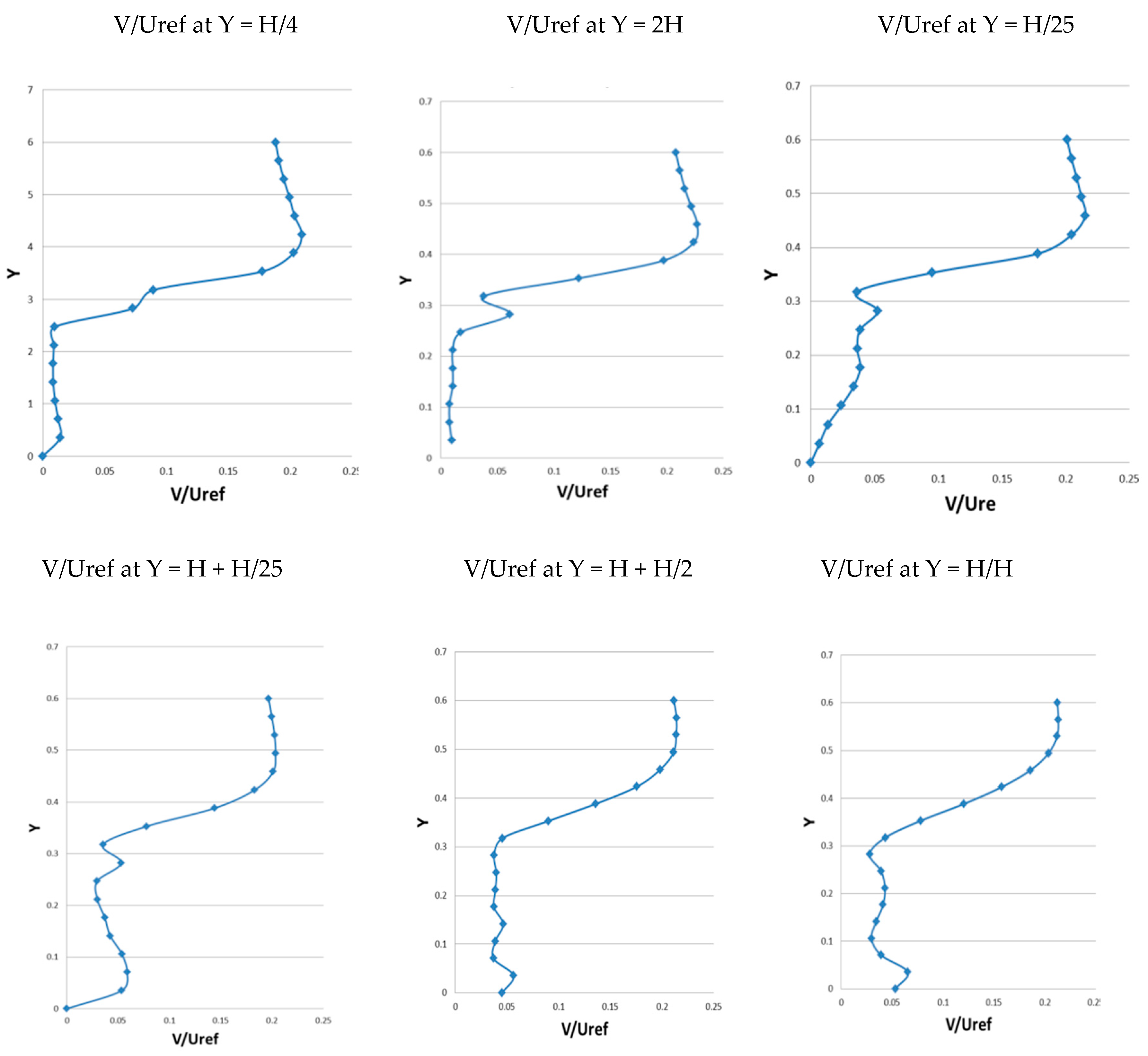
4. Model Validation
5. Results and Discussion
5.1. Container House Natural Ventilation Analysis
5.2. Analysis of Natural Ventilation Contour Plot of the Container House
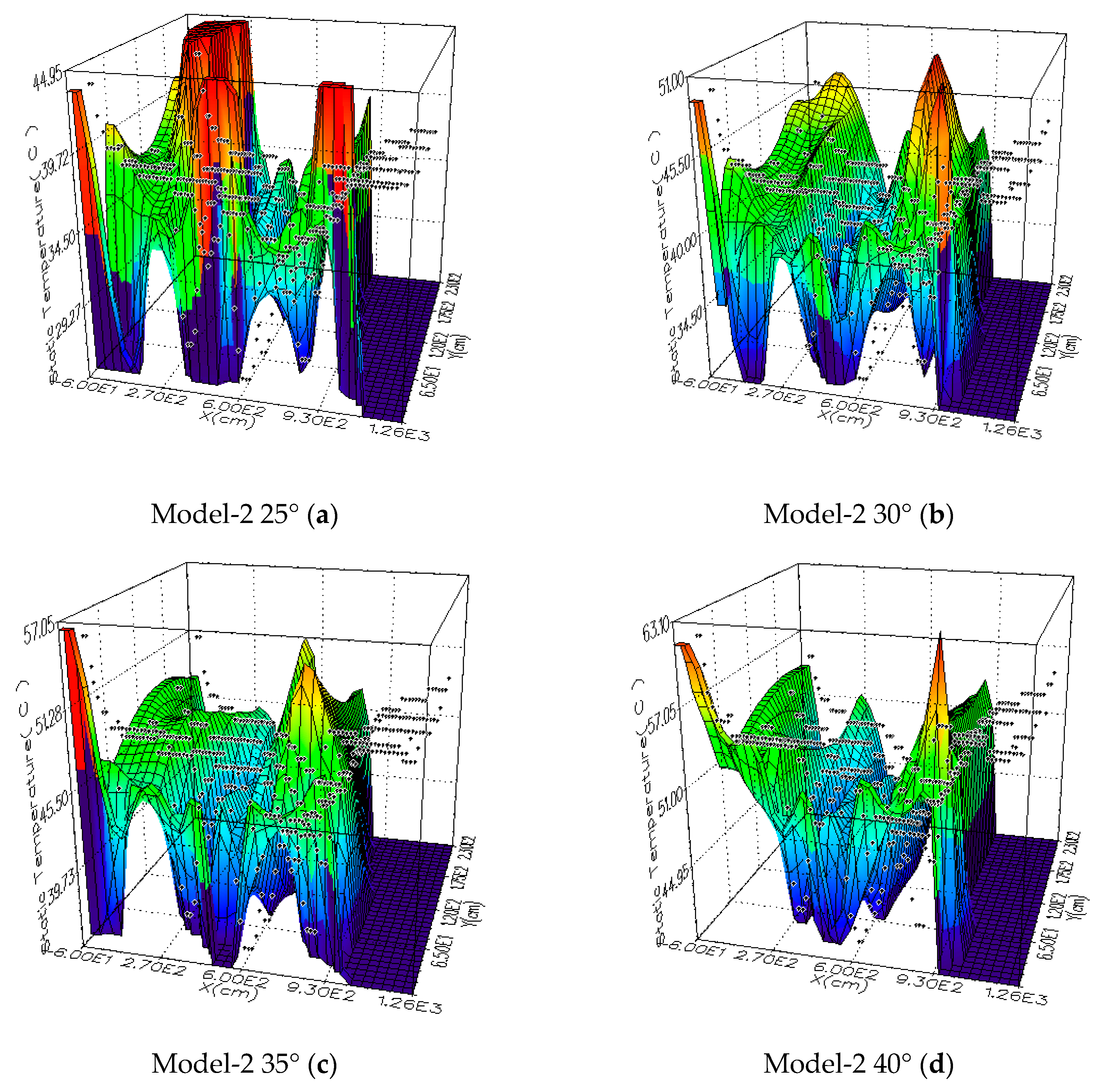
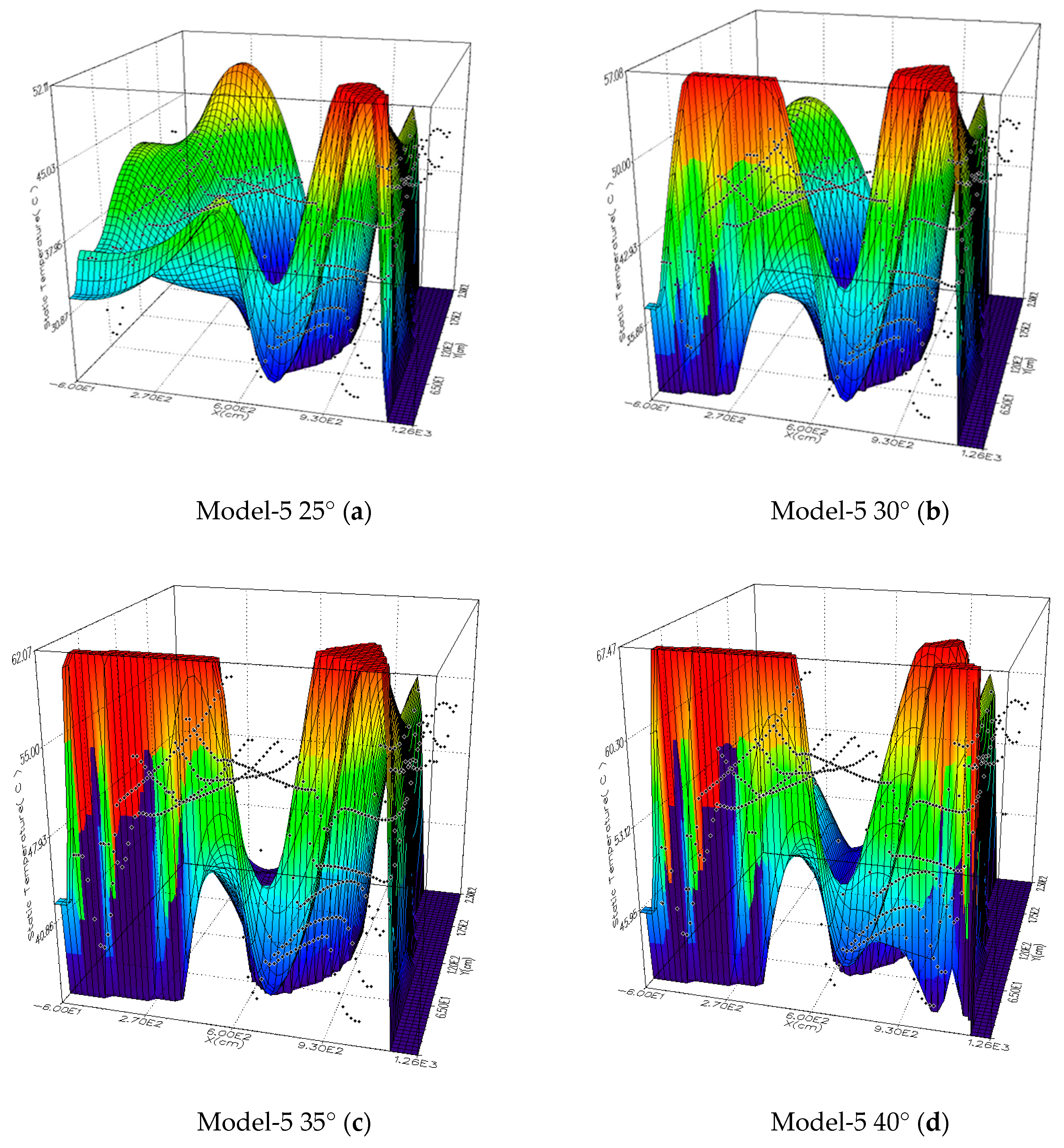
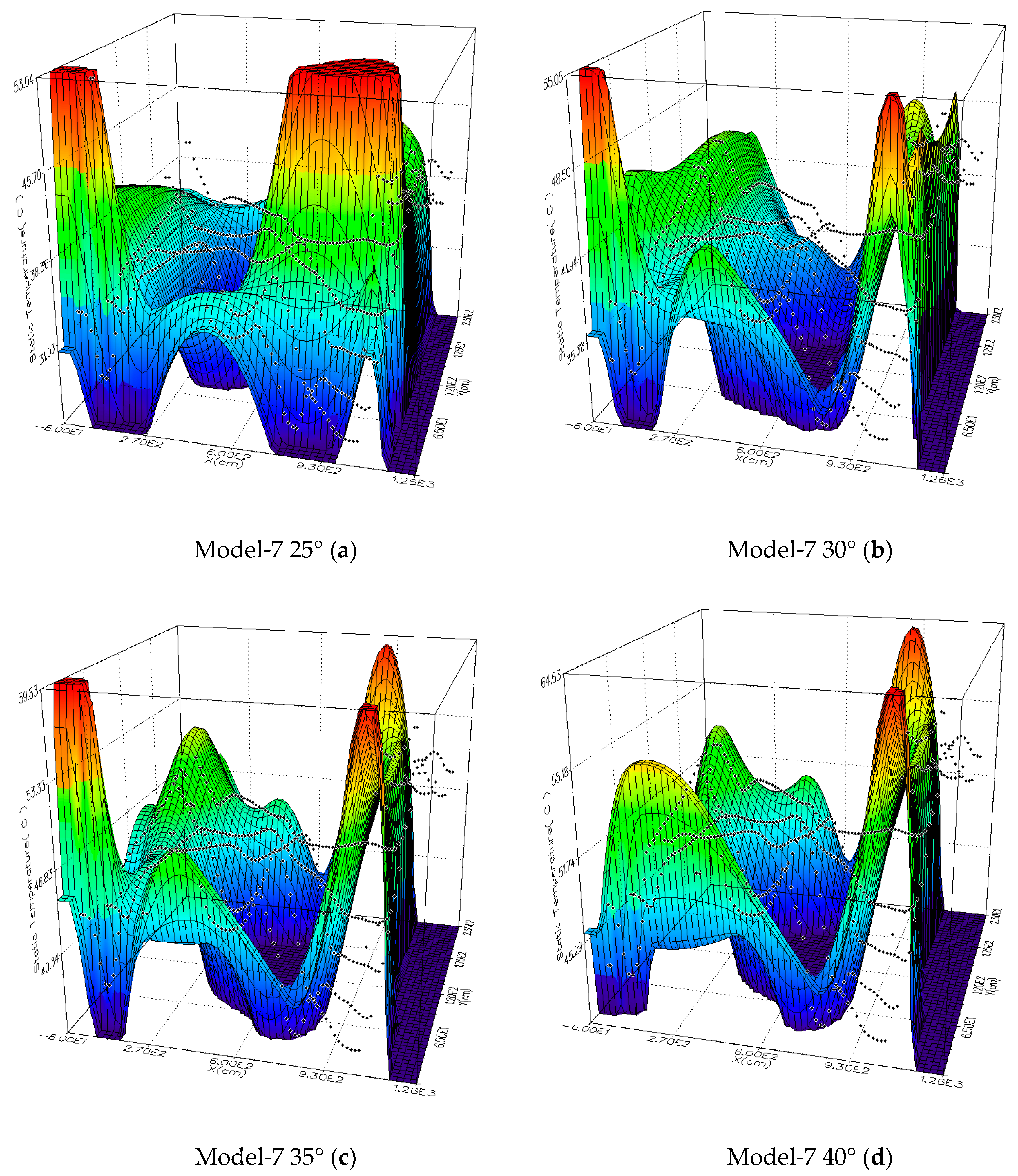
5.3. Analysis of Solar Radiation Thermal Field in the Container House
5.4. Comparative Curve Analysis of Solar Radiant Heat in the Container House
5.5. Analysis of Temperature Change and Wind Velocity Change in the Container House
6. Conclusions
- I.
- The experimental results, which are quite close to the CFD prediction, confirm that the eight models form a good prediction of the simple configuration of the container house and indoor airflow.
- II.
- In terms of the ventilation and indoor airflow patterns under different configurations of windows and doors, the effect of model 3 is the best, and this effect is very significant. In terms of indoor wind velocity, under the asymmetry of wind velocity of asymmetric windows, and under the comparison with the thermal effects taken away by ventilation and airflow, the gaps of air quality and thermal comfort are shown by the analysis model. When the volumes of the container houses are the same and the velocity is consistent with the solar radiant heat, there is a 10% gap in the maximum flow velocity between the models.
- III.
- Temporary use of container houses plays an important role in this study. When the ambient temperature increases, the airflow velocity of natural ventilation increases, and the effect of the window configuration position is seen, indoor airflow depends on various parameters and characteristics of the incoming air flow, therefore, when the indoor airflow is analyzed, many design changes are also analyzed at the same time, such as the potential of natural ventilation and cooling temperature field.
- IV.
- It is found from the study that the wind velocity at the window outlet can also be increased by the natural ventilation of the door at the entrance, which can increase the natural ventilation velocity of the outlet window, and the airflow generated by the door ventilation opening in the house can take away a large amount of radiant heat air movement.
- V.
- The study results show that the configuration position of the inlet and outlet sections of the container house can improve the efficiency of natural ventilation, so the results show that when the temperature is 25 degrees, the indoor thermal environment temperature at the central position of model 3 decreases the benefit by 35% that of model 8, which can illustrate that 300 cm–900 cm is the optimal position for thermal comfort in the activity area of the container house.
- VI.
- Among various types of container houses, model 3 can achieve the optimal effect, its sunshine environment is 1041 W/m2, while the living environment temperature in container houses is within 45 °C, which is acceptable to the human body.
Author Contributions
Funding
Conflicts of Interest
References
- Yi, J.; Donald, A.; Huw, J.; Rob, A.; Chen, Q. Natural ventilation in buildings: Measurement in a wind tunnel and numerical imulation with large-eddy simulation. J. Wind Eng. Ind. Aerodyn. 2003, 91, 331–353. [Google Scholar]
- Allocca, C.; Chen, Q.; Leon, R. Glicksman Design analysis of single-sided natural ventilation. Energy Build. 2003, 35, 785–795. [Google Scholar] [CrossRef]
- Menassa, C.C.; Taylor, N.; Nelson, J. Optimizing hybrid ventilation in public spaces of complex buildings e A case study of the Wisconsin Institutes for Discovery. Build. Environ. 2013, 61, 57–68. [Google Scholar] [CrossRef]
- Kobayashi, T.; Chikamoto, T.; Osada, K. Evaluation of ventilation performance of monitor roof in residential area based on simplified estimation and CFD analysis. Build. Environ. 2013, 63, 20–30. [Google Scholar] [CrossRef]
- Lim, C.H.; Omidreza, S.; Sulaiman, M.Y.; Kamaruzzaman, S.M. Empirical study of a wind-induced natural ventilation tower under hot and humid climatic conditions Sopian. Energy Build. 2012, 52, 28–38. [Google Scholar]
- Bangalee, M.Z.I.; Lin, S.Y.; Miau, J.J. Wind driven natural ventilation through multiple windows of a building: A computational approach. Energy Build. 2012, 45, 317–325. [Google Scholar] [CrossRef]
- Adamu, Z.A.; Price, A.D.F.; Cook, M.J. Performance evaluation of natural ventilation strategies for hospital wards e A case study of Great Ormond Street Hospital. Build. Environ. 2012, 56, 211–222. [Google Scholar] [CrossRef]
- Prajongsan, P.; Sharples, S. Enhancing natural ventilation, thermal comfort and energy savings in high-rise residential buildings in Bangkok through the use of ventilation shafts. Build. Environ. 2012, 50, 104–113. [Google Scholar] [CrossRef]
- Wang, H.; Chen, Q. A new empirical model for predicting single-sided, wind-driven natural ventilation in buildings. Energy Build. 2012, 54, 386–394. [Google Scholar] [CrossRef]
- Gao, C.F.; Lee, W.L. Evaluating the influence of openings configuration on natural ventilation performance of residential units in Hong Kong. Build. Environ. 2012, 46, 961–969. [Google Scholar] [CrossRef]
- Bu, Z.; Kato, S.; Takahashi, T. Wind tunnel experiments on wind-induced natural ventilation rate in residential basements with areaway space. Build. Environ. 2012, 45, 2263–2272. [Google Scholar] [CrossRef]
- Khanal, R.; Lei, C. Solar chimney—A passive strategy for natural ventilation. Energy Build. 2011, 43, 1811–1819. [Google Scholar] [CrossRef]
- Gan, G. General expressions for the calculation of air flow and heat transfer rates in tall ventilation cavities. Build. Environ. 2011, 46, 2069–2080. [Google Scholar] [CrossRef]
- Cheung, J.O.P.; Liu, C.H. CFD simulations of natural ventilation behaviour in high-rise buildings in regular and staggered arrangements at various spacings. Energy Build. 2011, 43, 1149–1158. [Google Scholar] [CrossRef]
- Gan, G. Impact of computational domain on the prediction of buoyancy-driven ventilation cooling. Build. Environ. 2010, 45, 1173–1183. [Google Scholar] [CrossRef]
- Olivera, E.D.; Topisirovic, G. Energy efficiency optimization of combined ventilation systems in livestock buildings. Energy Build. 2010, 42, 1165–1171. [Google Scholar]
- Wang, X.; Huang, C.; Cao, W. Mathematical modeling and experimental study on vertical temperature distribution of hybrid ventilation in an atrium building. Energy Build. 2009, 41, 907–914. [Google Scholar] [CrossRef]
- Hughes, B.R.; Abdul Ghani, S.A.A. Investigation of a windvent passive ventilation device against current fresh air supply recommendations. Energy Build. 2008, 40, 1651–1659. [Google Scholar] [CrossRef]
- Gratia, E.; Herde, A.D. Guidelines for improving natural daytime ventilation in an office building with a double-skin facade. Sol. Energy 2007, 81, 435–448. [Google Scholar] [CrossRef]
- Wang, L.; Wong, N.H. The impacts of ventilation strategies and facade on indoor thermal environment for naturally ventilated residential buildings in Singapore. Build. Environ. 2007, 42, 4006–4015. [Google Scholar]
- Tahir, A.; Osman, Y. Investigating the potential use of natural ventilation in new building designs in Turkey. Energy Build. 2006, 38, 959–963. [Google Scholar]
- Janjai, S.; Itsara, M.; Jarungsaeng, L. Satellite-derived solar resource maps for Myanmar. Renew. Energy 2013, 53, 132–140. [Google Scholar] [CrossRef]
- Ramkumar, J.; Douglas, L.M. Temporal and Spatial Variations of the Solar Radiation Observed in Singapore. Energy Procedia 2012, 25, 108–117. [Google Scholar]
- Pramod, K.P.; Michelle, L.S. A new method to estimate average hourly global solar radiation on the horizontal surface. Atmos. Res. 2012, 114, 83–90. [Google Scholar]
- Matthew, T.D.; Richard, P.C. Solar UV variations during the decline of Cycle 23. J. Atmos. Sol. Terr. Phys. 2012, 77, 225–234. [Google Scholar]
- Ibrahim, S.; Daut, I.; Irwan, Y.M.; Irwant, M.; Gomesh, N.; Razliana, A.R.N. An Estimation of Solar Radiation using Robust Linear Regression Method. Energy Procedia 2012, 18, 1413–1420. [Google Scholar] [CrossRef]
- Journée, M.; Bertrand, C. Improving the spatio-temporal distribution of surface solar radiation data by merging ground and satellite measurements. Remote Sens. Environ. 2010, 114, 2692–2704. [Google Scholar] [CrossRef]
- Islam, M.D.; Alili, A.A.; Kubo, I.; Ohadi, M. Measurement of solar-energy (direct beam radiation) in Abu Dhabi, UAE. Renew. Energy 2010, 35, 515–519. [Google Scholar] [CrossRef]
- Hu, L.; Yan, B.; Wu, X.; Li, J. Calculation method for sunshine duration in canopy gaps and its application in analyzing gap light regimes. For. Ecol. Manag. 2010, 259, 350–359. [Google Scholar] [CrossRef]
- Gastli, A.; Charabi, Y. Solar electricity prospects in Oman using GIS-based solar radiation maps. Renew. Sustain. Energy Rev. 2010, 14, 790–797. [Google Scholar] [CrossRef]
- Bulut, H. Typical solar radiation year for southeastern Anatolia. Renew. Energy 2004, 29, 1477–1488. [Google Scholar] [CrossRef]
- Zhou, P.; Qian, W.H. Adding draft angle to B-spline and NURBS surfaces. Comput. Aided Des. 2012, 44, 617–625. [Google Scholar] [CrossRef]
- Jala, A.; Kamal, S.; Kim, D. Depth Silhouettes Context: A new robust feature for human tracking and activity recognition based on embedded HMMs. In Proceedings of the 12th International Conference on Ubiquitous Robots and Ambient Intelligence (URAI), Goyang, Korea, 28–30 October 2015; pp. 294–299. [Google Scholar] [CrossRef]
- Jalal, A.; Kim, J.T.; Kim, T.S. Development of a life logging system via depth imaging-based human activity recognition for smart homes. Proc. Int. Symp. Sustain. Healthy Build. 2012, 19, 91–95. [Google Scholar]
- Lu, H.P.; Lin, H.H. Exploring the Impact of Intuitive Thinking on Creativity with Gray Relational Analysis. Sustainability 2020, 12, 2989. [Google Scholar] [CrossRef]
- Lin, H.H. Improvement of Human Thermal Comfort by Optimizing the Airflow Induced by a Ceiling Fan. Sustainability 2019, 11, 3370. [Google Scholar] [CrossRef]
- Lin, H.H.; Cheng, J.H.; Chen, C.H. Application of Gray Relational Analysis and Computational Fluid Dynamics to the Statistical Techniques of Product Designs. Symmetry 2020, 12, 227. [Google Scholar] [CrossRef]


| Container house size | 12.19 m long/2.44 m wide/2.59 m high |
| window | 67 cm × 67 cm |
| Door | 120 cm × 210 cm |
| cm | Window 1 | Window 2 | Window 3 | Window 4 | Door |
|---|---|---|---|---|---|
| Model-1 | X80/Y0/Z95.5 | X1060/Y0/Z95.5 | X330/Y235/Z95.5 | X810/Y235/Z95.5 | X550/Y0/Z20 |
| Model-2 | X330/Y0/Z95.5 | X810/Y0/Z95.5 | X330/Y235/Z95.5 | X810/Y235/Z95.5 | X550/Y0/Z20 |
| Model-3 | X330/Y0/Z95.5 | X810/Y0/Z95.5 | X80/Y235/Z95.5 | X1060/Y235/Z95.5 | X550/Y0/Z20 |
| Model-4 | X80/Y0/Z95.5 | X1060/Y0/Z95.5 | X80/Y235/Z95.5 | X1060/Y235/Z95. | X550/Y0/Z20 |
| Model-5 | X80/Y0/Z95.5 | X610/Y0/Z95.5 | X80/Y235/Z95.5 | X610/Y235/Z95.5 | X940/Y0/Z20 |
| Model-6 | X80/Y0/Z95.5 | X360/Y0/Z95.5 | X80/Y235/Z95.5 | X360/Y235/Z95.5 | X940/Y0/Z20 |
| Model-7 | X80/Y0/Z95.5 | X760/Y0/Z95.5 | X80/Y235/Z95.5 | X760/Y235/Z95.5 | X940/Y0/Z20 |
| Model-8 | X430/Y0/Z95.5 | X760/Y0/Z95.5 | X430/Y235/Z95.5 | X760/Y235/Z95.5 | X940/Y0/Z20 |
| Equation | ψ |
| Continuity | 1 |
| X-momentum | u |
| Y-momentum | v |
| Z-momentum | w |
| Energy | I or T |
| 1.44 | 1.92 | 0.09 | 1.0 | 1.3 |
| ventilation | Inlet boundary condition | Input = opening width (m), air temperature: 25 °C/30 °C/35 °C/40°C (°C), and inflow velocity:10 m/s |
| Outlet boundary condition | No sliding condition | |
| Outlet | Outlet static pressure is 0 | |
| Wall, radiant surface | speed | Generalized record file method, no sliding condition |
| Solar axis radiation heat | In the literature, the maximum instantaneous radiant energy falling on the surface during the summer heat can be estimated by 1041 W/m2 [22,23,31]. The surface temperature is determined on the solid surface, and thermal equilibrium is simulated through radiation and conduction. The convective heat transfer coefficient is fixed on the radiation surface: 1000.0 [W/(m2 °C)] | |
| Humidity | Radiation surface: AH (absolute humidity) gives the corresponding saturated vapor pressure, the surface temperature of the radiation cooling surface is lower than the dew point temperature of air, water vapor condensation occurs, in other cases, AH = 0. Humidity heat transfer coefficient is calculated. | |
| Surface emissivity | Wall: 0.9, symmetric plane: 0.0 | |
| Grid system | Grid: 560,000 control volumes with minimum control quantity of 1 |
| Model-1 | Model-2 | Model-3 | Model-4 | Model-5 | Model-6 | Model-7 | Model-8 | |
|---|---|---|---|---|---|---|---|---|
| Air volume at 25 °C | 6.79 | 6.34 | 6.82 | 6.78 | 6.33 | 6.54 | 6.64 | 6.33 |
| Air volume at 40 °C | 6.93 | 6.43 | 6.89 | 6.95 | 7.02 | 6.63 | 6.69 | 6.42 |
Publisher’s Note: MDPI stays neutral with regard to jurisdictional claims in published maps and institutional affiliations. |
© 2020 by the authors. Licensee MDPI, Basel, Switzerland. This article is an open access article distributed under the terms and conditions of the Creative Commons Attribution (CC BY) license (http://creativecommons.org/licenses/by/4.0/).
Share and Cite
Lin, H.-H.; Cheng, J.-H. A Study of the Simulation and Analysis of the Flow Field of Natural Convection for a Container House. Sustainability 2020, 12, 9845. https://doi.org/10.3390/su12239845
Lin H-H, Cheng J-H. A Study of the Simulation and Analysis of the Flow Field of Natural Convection for a Container House. Sustainability. 2020; 12(23):9845. https://doi.org/10.3390/su12239845
Chicago/Turabian StyleLin, Hsin-Hung, and Jui-Hung Cheng. 2020. "A Study of the Simulation and Analysis of the Flow Field of Natural Convection for a Container House" Sustainability 12, no. 23: 9845. https://doi.org/10.3390/su12239845
APA StyleLin, H.-H., & Cheng, J.-H. (2020). A Study of the Simulation and Analysis of the Flow Field of Natural Convection for a Container House. Sustainability, 12(23), 9845. https://doi.org/10.3390/su12239845