Article

Automatic Development of Deep Learning Architectures for Image Segmentation

by
Sergiu Cosmin Nistor
*,
Tudor Alexandru Ileni
and
Adrian Sergiu Dărăbant
Department of Computer Science, Babeș-Bolyai University, 400084 Cluj-Napoca, Romania
*
Author to whom correspondence should be addressed.
Sustainability 2020, 12(22), 9707; https://doi.org/10.3390/su12229707
Submission received: 29 October 2020 / Accepted: 16 November 2020 / Published: 20 November 2020

Abstract

:
Machine learning is a branch of artificial intelligence that has gained a lot of traction in the last years due to advances in deep neural networks. These algorithms can be used to process large quantities of data, which would be impossible to handle manually. Often, the algorithms and methods needed for solving these tasks are problem dependent. We propose an automatic method for creating new convolutional neural network architectures which are specifically designed to solve a given problem. We describe our method in detail and we explain its reduced carbon footprint, computation time and cost compared to a manual approach. Our method uses a rewarding mechanism for creating networks with good performance and so gradually improves its architecture proposals. The application for the algorithm that we chose for this paper is segmentation of eyeglasses from images, but our method is applicable, to a larger or lesser extent, to any image processing task. We present and discuss our results, including the architecture that obtained 0.9683 intersection-over-union (IOU) score on our most complex dataset.

1. Introduction

The large quantity of data which is constantly generated provides a great opportunity to study various phenomena, obtain insights and use the gained knowledge to improve our solutions to tasks in various domains. This great opportunity is also a great challenge as the quantities of data are vast and are very difficult to process, aggregate and synthesize into useful information.
Artificial intelligence is a promising solution for processing all of this data. Automatic methods can be developed and then applied to different tasks. Even so, machine learning algorithms must be tailored to the data they are required to process. As the inputs have many forms and the tasks are very diverse, many different such algorithms must be elaborated. This development requires many resources, especially human resources and time.
A new type of algorithm starts to emerge for the purpose of finding these solutions in an automatic manner: Neural Architecture Search (NAS). As many tasks can be solved with different deep learning algorithms, the important decision which must be made is the architecture of the network that will be trained to solve the problem. The proposed new algorithms search for such architectures and discover increasingly better solutions.
We propose, in this paper, our own flavor of the neural architecture search algorithm. We use a recurrent neural network to generate convolutional neural network (CNN) architectures for specific problems. CNNs are deep learning algorithms that already obtained great results on many computer vision tasks [1,2,3,4,5,6]. In practice, a neural architecture is created in a tedious manual approach where researchers try to find building blocks, new loss functions, improved optimizers, etc in an iterative process where the partially discovered network is always fully trained as elements are added to it. This process not only takes time but is also computationally hungry. As we want our algorithm to work as fast as possible and use as little resources as possible, we only search for small building blocks which we then assemble into full architectures. Our proposer explores a space of assembled small network building blocks, searches for networks that obtain good results on the task that we considered, and is rewarded when finding high-performing architectures.
To give a definition, the classification is the task of deciding if an image contains an object; the detection is the task of identifying the object position (bounding box) in the image; the semantic segmentation is the individual pixel classification, to get the actual area of each object in the image; and the instance segmentation is the pixel classification and bounding box detection. Pixel classification is a very researched topic in computer vision, with solutions based on semi-supervised learning [7], fully convolutional architectures [8], or encoder-decoder approaches [9]. They are vastly applied in fields like autonomous driving [10], biomedical image analysis [9] or scene recognition [11].
We considered an image segmentation task to be solved by our neural architecture search algorithm. Given images that contain eyeglasses, we wish to isolate only the pixels that represent the eyeglasses and ignore the background. A possible real world scenario is to use the frame masks to obtain a digital eyeglasses database. By tacking a picture of the eyeglasses frames, and eliminating the background we can use the frames-only images for digital try-on solutions. This mechanism can enable users to “try” a pair of eyeglasses from the comfort of their homes.
The rest of this paper is structured as follows: in Section 2 we present the methods on which we based our algorithm and we describe the proposed neural architecture search approach that we took. Section 3 is dedicated to describing the task which we wish to solve and presenting our results. We report in this section numerical results and we describe the best-performing architecture that we discovered. We draw our conclusions and present further research directions in Section 4.

2. Materials and Methods

In this section we first present the work on which we based our solution and experiments and then we describe the solution that we propose for an automatic search for new convolutional neural network architectures.

2.1. Related Work

As computer science progresses, more and more domains take advantage of the power of computing. Applications of computer science can be found in communication [12,13], finance [14], education [15], healthcare [16,17], management [18] and many more. As the quantity and variety of data increases, there is a need for more artificial intelligence algorithms to process this data. Machine learning algorithms need to be tailored specifically to each task and it is difficult to handcraft algorithms for each problem. Automatic methods of creating algorithms for solving each task are a possible solution.
While earlier CNN architectures consisted of convolutional and pooling layers simply stacked on top of each other [19,20], newer architectures included reusable modules, or CNN cells, which are more complex structures, yet still small, that can be the building blocks of a full CNN architecture [21,22,23,24].
As CNNs were used more and more in various domains, it became clear that handcrafting an architecture which obtains the best results on every task is very challenging. Different architectures obtain results for different problems and obtaining the best performance on a task using a certain CNN does not necessarily imply obtaining the best performance on another given task. A possible solution is to handcraft an architecture for every problem, but this is very demanding. Researchers must try various configurations, study the results, and decide what modifications must be made. This is very time-consuming and requires many people working for solving the many computer vision tasks.
Another solution is to automate the architecture search process. NAS algorithms aim to automatically find an efficient architecture for solving a given task. As described by Elsken et al. [25] a NAS algorithm has three main components: search space, search strategy, and performance estimation strategy. The search space is the set of all possible architectures that the method considers. This space is usually defined by the representation of the solutions and the constrictions imposed on them.
As this space is very large for most NAS algorithms, a method for “traversing” this space in an efficient way is necessary. This is the search strategy. For example, using random search is not appropriate as it would not take advantage of the previously explored and evaluated architectures. All potential architectures would have an equal proposal probability-yielding thus a low improvement chance for the overall solution. Other, more sophisticated, strategies use the experience gained during the analysis of the subspace that was done such that the direction of the search is selected in a way that the chance of improving the solution is greater. There were proposed NAS algorithms which use for the search strategy evolutionary algorithms [25], reinforcement learning [26,27,28,29,30] or fully-differentiable methods [31,32].
Each search strategy has its own challenges. Evolutionary algorithms require large populations of individuals, which in the case of NAS algorithms would represent the architecture descriptions. A particularly challenging task is to create crossover operators that would take two architectures and create a single architecture from them while preserving the useful structural elements of each “parent” architecture. Fully-differentiable methods require training super-networks, which are very large, use many learnable parameters, make many computations and hence require high computational resources to train.
Finding an efficient architecture for a task may imply evaluating a very large number of designs, this may cause NAS algorithms to be highly demanding in computing resources. If every evaluated architecture would be completely trained, the NAS algorithm may take impractical periods of time to run or need a very large number of computing units. To diminish this problem, NAS performance estimation strategies are employed. These strategies are given a design and estimate how well this design will be able to solve the task without completely training it.
Reinforcement learning is a method of training machine learning algorithms based on how well they are able to accomplish what is required of them. In supervised training scenarios, for each input, the expected output is known and the machine learning algorithm is taught to make these associations and penalized when it fails to do so. Unfortunately, not all problems have a known correct answer. Reinforcement learning scenarios can be applied in such cases, provided there is a measure of the quality of the given answer. The model is given the input, produces the output and this output is then processed by a reward function which is greater if the answer has a good quality or lower if the answer is not appropriate.
The NAS algorithm proposes an architecture and the reward is the performance of the architecture on the given task. As previously mentioned, the exact performance can be difficult to always calculate given a long time required and a large number of architectures to evaluate. Because of this reason, the performance estimation is used as a reward function.
There are already multiple NAS approaches based on reinforcement learning. Baker et al. [26] proposed a NAS algorithm that searches for full CNN architectures. The representation of a possible architecture is a sequence of layers, each one falling in one of these categories: convolutional, pooling, fully-connected, global average pooling or softmax. For the search space, they modeled the problem as a Markov chain. The initial state represents an empty architecture and the transition to each following state implies the addition of a new layer to the CNN. A type of reinforcement learning, Q-Learning, was used to guide the search. Each discovered CNN was trained on three image processing datasets. One of these is the CIFAR-10 dataset [33], a popular option for testing NAS algorithms because its complexity is not that large. The accuracy on the validation sets is taken as performance estimation.
Zoph et al. [27] propose another NAS algorithm in which full CNN architectures are searched for. The networks are again a sequence of layers, but these layers may also have skip-connections [34]. If the dimensions of the two layers concatenated by the skip-connection do not coincide, the smaller one is padded. The convolutional layers have a set of characteristics: filter height, filter weight, stride height, stride width, and a number of filters. A “controller RNN” is used for proposing CNN architectures. At each generation step, this controller describes the next layer with all of its characteristics. For the skip-layers, a feed-forward layer takes as input the hidden state of the controller at the current step and at each previous step, deciding if a connection is made.
For training the controller, Zoph et al. [27] use reinforcement learning, more exactly, policy gradient. At each training step, multiple CNN architectures are proposed and trained on CIFAR-10 for a fixed number of steps. The best performing one is retrained until it converges and its final accuracy on the validation set is taken as the reward. This NAS solution is highly resource-demanding, as 800 networks are trained in parallel on 800 GPUs at any time of a run of this algorithm.
Zoph et al. [28] built on the solution from [27]. In this new iteration of the NAS algorithm, the search space does not contain full CNN architectures, but CNN cells. The algorithm searches for a smaller structure that is then used to create a full CNN architecture by stacking multiple such structures. Each cell is composed of 5 “blocks”. Each block takes as input the outputs of two previous blocks, applies an operation on them and then combines them. The possible operations are various convolutional or pooling operations. The combination is done either by element-wise addition or concatenation. As the input blocks, the input of the cell may also be taken.
For describing the cells, a controller RNN is used in [28]. Pairs of two cells are generated at each step: one “Normal Cell” and one “Reduction Cell”, the difference being that the first preserves the width and height of the input, while the second reduces it. Based in these pairs, full CNN architectures are built by stacking multiple cells of each type. The controller RNN generates multiple pairs for which the full CNNs are trained on CIFAR-10 and evaluated and the best result is used as reward for reinforcement learning.
Another interesting approach is taken in [35], where an exhaustive search is attempted. The method only trains a few CNN cells and predicts the performance of the others based on the evaluated ones. In this NAS algorithm, cells of increasing size are discovered, as the search progresses.

2.2. Proposed Solution

In this subsection, we describe the method that we propose for developing new convolutional neural network architectures. The proposed solution is to automatically generate CNN architectures by inferring task specific CNN sub-part cell architectures (Figure 11) and integrating them into a larger CNN template (as presented in Figures 9 and 10). For generating the cells, we use a proposer model based on a RNN, which we train using reinforcement learning.
A cell is a small CNN sub-part composed of nodes. Each node is a computational unit that aggregates data and applies an operation. A cell can be instantiated multiple times when building the full CNN architecture and each such instance may/will have a different number of filters. We chose the cell sub-part generation approach as opposed to proposing entire full sized CNNs as the search space that needs to be explored differs by orders of magnitude. We start from the assumption that generating a task-efficient cell and assembling its instances in a larger architecture would transfer the cell good properties to the fully assembled CNN. This approach allows the proposer model to focus on smaller, yet more complex individual sub-part structures that can be reused in the full CNN architecture. While proposing the entire network architecture gives the algorithm the freedom to describe the full CNN, the large search space is difficult to explore and the proposer model is less likely to find an efficient solution. At the same time, approaches that search for the full architecture are very resource-demanding and allow only very simple structures in the network, like sequences of convolutional and pooling layers and sometimes skip-connections [26,27].
We propose CNN cells and integrate them into larger architectures. Once a cell is generated by the RNN, we compose a CNN by using multiple head-to-tail instances of this cell, with various numbers of filters, according to a template we describe for the particular problem we need to solve. In this way, the solutions that we propose are configurable and reusable. Depending on the complexity of the task, deeper or shallower CNN architectures can be created by integrating varying number of instances of the discovered cell, much like in a LEGO game.
Our representation of the cell is a directed acyclic graph (DAG). The cell consists of an input node, an output node, and intermediary nodes. The input node represents the input that is given to the cell. As multiple instances of the cell are used in the full CNN architecture, the input can be received from different sources. For example, if the cell is right at the beginning of the CNN, then the input node will be the input image. If we have two consecutive cells in the network, the input node of the second cell will receive the data from the output node of the first cell.
Excepting the input node, each of the other nodes of the cell may receive the input from any number of the other nodes. To ensure that no cycles exist, we impose an ordering of the nodes, in which the first node is the input node and the last node is the output node, and we allow nodes to receive the input only from the nodes that are placed before in the ordering. The inputs from the nodes are concatenated on the depth dimension and an operation is applied for computing the output of the node.
The operations that we consider are the following:
  • 3 × 3 convolution
  • 1 × 1 convolution
  • 1 × 3 convolution followed by 3 × 1 convolution
  • 1 × 7 convolution followed by 7 × 1 convolution
  • 3 × 3 depthwise-separable convolution
  • 5 × 5 depthwise-separable convolution
  • 7 × 7 depthwise-separable convolution
  • 3 × 3 dilated convolution
For all convolutional layers, the activation function is rectified linear unit (ReLU). We chose these operations as they were proved to be useful for both handcrafted architectures [20,22,24] and architectures found with automatic methods [28,35]. Classical convolutional layers learn filters that have access to a region of the input, which is a compact slice, having a certain height and width and the depth equal to the depth of the input. This is the type of operations represented by the 3 × 3 and 1 × 1 convolutions. The pairs of 1 × 3, 3 × 1 and 1 × 7, 7 × 1 convolutions preserve the receptive field of the 3 × 3 and 7 × 7 convolutions respectively while using a lower number of learnable parameters.
A depthwise-separable convolution [36] is another variation which preserves the receptive field while lowering the number of parameters. In this case, if we consider an A × B convolution, the first step is to apply filters of size A × B × 1, meaning that each filter will have access only to one slice in the depth of the input. The second step is to apply a classical convolution of size 1 × 1, which has access to the entire depth of the input.
A dilated convolution [37,38] will skip some inputs. In our case for a 3 × 3 dilated convolution, for each value in the output, 3 × 3 values of each depth slice of the input are considered, but these values are not consecutive. They are taken from a 5 × 5 input where only the first and then every second value is considered. This process goes on both axes, having only 3 × 3 values taken by the computation.
The number of filters of our cell is configurable to allow different instances of the cell to have different numbers of filters. Cells closer to the input of the full CNN architecture should have fewer filters, while cells placed in the middle of the architecture should have a higher number of filters. Each node in a given cell is an independent computational unit, but in our approach, they have the same number of filters for all nodes in a cell to make the cell homogeneous.
While there are other works that represent a cell similarly to our definition, most fix a number of nodes from which the input is taken. For example, in [28,29] each node takes inputs from exactly two preceding nodes. We consider that allowing the proposing algorithm to select more inputs for each node gives it greater flexibility. By fixing the number of the inputs, to represent the same cell would require a larger number of nodes and including the identity operation. Our approach allows greater flexibility by having a variable number of inputs and also allows skip-connections similar to residual networks [34] inside the cells.
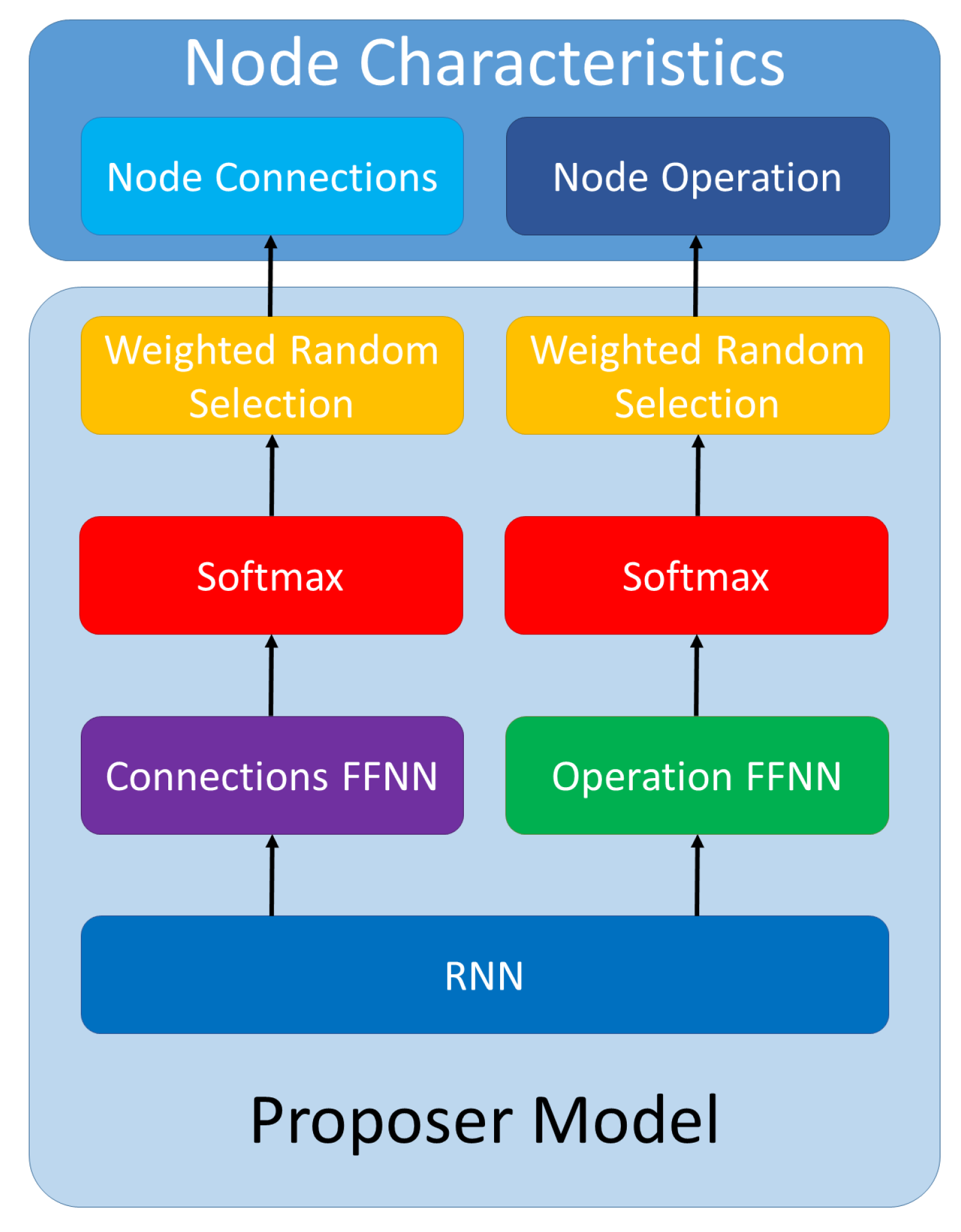
For proposing the networks we use a recurrent neural network (RNN). For each CNN cell, the proposer network will generate the characteristics of each component node: the nodes from which it takes input and the operation that it applies. The proposer RNN generates each node directly in the order used for assuring the DAG property, so the last generated node is the output node. From our perspective, a cell (as a DAG) is a sequential entity and hence we model it by using a RNN [39]. As there is no information to be generated for the input node, the cell description starts with the first intermediary node.
The proposer RNN has two layers of 32 Gated Recurrent Units (GRUs) [40]. The output of the last recurrent layer is processed by two feed-forward neural networks (FFNNs): one for the input nodes and one for the operation. The FFNNs each consist of two layers of 32 units with ReLU activation and one additional final layer for making the prediction. The final layer of the FFNN has two units for each node. They are used to decide whether the node is taken as input or not. The corresponding node operation is decided in the final layer of the FFNN using one unit for each potential operation.
When deciding each characteristic (operations and connections) of the node, the outputs are passed through a softmax operation and the results are used as probabilities for weighted random selection. We do this selection for encouraging the proposer to explore more of the search space. As the random selection is weighted using the softmax probabilities, characteristics which the RNN considers more appropriate have a higher chance of being selected, while other options have a smaller chance of being selected.
A graphical representation of the proposer network generating the characteristics of a node can be seen in Figure 1.
When describing a CNN cell, the number of nodes is known from the start. As we do not want to limit our method to a predefined number of nodes, we increment the number of nodes during the training of the RNN such that it will propose cells with different dimensions.
Figure 2 contains an example of the visual representation of the proposal of a CNN cell which consists of the input node and three other nodes. For each node, the RNN model generates the characteristics. The characteristics of each node are then fed back as input to the proposer network so that the next node can be generated in a recurrent manner. With red arrows, we represent the recurrent connections, as the state of the RNN is updated and used at each step. The connections of each node are to the ones with a strictly lower identifier, as the index in the node ordering that assures the DAG property. The input node has 0 as identifier. Each operation has an operation identifier.
For training our proposer network, we use reinforcement learning (RL). At each training step, the RNN will propose a cell. For each cell, we build a full CNN by integrating multiple instances of the cell in a predefined evaluation architecture template and partially train it on a task. The templates that we used for our specific task are described in Section 3.2. The network is then evaluated on this task and the metric is used as the performance score of the cell.
As we do not have a priori (ground truth) training data, we train the proposer RNN in a synthetic auto-feedback loop. We generate cells, we estimate their performance and we use the RL rewards as feedback. The feedback is implemented as a gradient scaling process. The generated cells become thus training data and the rewards become a form of learning rate. As we want to direct the proposer towards efficient designs, we scale the gradients with the rewards computed as in Equation (1) such that the network is encouraged to make decisions similar to the ones that led to high-performance architectures. We compute the loss between the softmax probabilities generated by the proposer and the representation of the cell. As the loss function, we use cross-entropy. As an example, if the proposer would give the score 0.85 in favor of establishing a connection between two particular nodes and 0.15 against it and the final decision was to create the connection, the values used for computing the loss would be (0.15, 0.85) as the prediction and (0, 1) as the ground truth.
Because training a deep network on a large dataset requires many computational resources, we employ a performance estimation strategy. Firstly, the CNN constructed at this phase is small, so that a forward pass takes very little time and each training step is completed quickly. Secondly, in this evaluation phase we do not use the full dataset which contains large-size images of the task at hand, but derive a dataset of smaller-size images that are faster to process. The CNN is trained for a fixed number of epochs and then it is evaluated.
At this stage, we are not interested in an absolute performance metric of the architectures, but in the performance of the architectures relative to one another. A hint on this decisions would be the fact that the template evaluation networks built from the generated cells have closely similar sizes and structure and training them for the same number of epochs would give an indication on their relative performance and guiding thus the proposer towards architectures of increasing quality. Using this approach allows us to estimate the performance of a cell much faster than a complete evaluation of its performance-which might not even be necessary at this step.
We compute the reward as in Equation (1) where s is the performance score of the cell.
R = exp ( s ) , s 0 , 1
In the beginning, the improvements might be larger as the proposer discovers what is generally useful for the task. We assume that the metric is directly proportional to the performance. As the training progresses, the performance metric increases slower. This is because increasingly finer improvements must be made to the cell architectures as better and better designs are generated. As a result, we have a system where the reward increases exponentially with the performance.
During the training of the proposer model, we start with cells consisting of a certain number of nodes. We train the RNN for a number of steps using this size, and then we increase by one the number of nodes. We repeat this process until we reach a superior limit that we establish for the size. By starting with a smaller size, the proposer has a smaller search space and can more easily find an efficient design. Gradually increasing the sizes of the cells increases the search space, giving the proposer the possibility to explore new options. This way the proposer starts with a smaller space to explore and with limited space jumps. While it trains itself in auto-feedback, the exploring space is dilated by increasing the number of nodes and the proposer is encouraged to use its past accumulated knowledge to explore it.
The cell size increase is implemented by extending the last layer of the Connections FFNN with two additional neurons that are used to decide if a connection exists from the last intermediary node to the nodes after it in the ordering. One neuron votes for keeping a connection, while the other votes for discarding the connection. The higher score imposes the final decision, allowing thus the architecture to evolve. While training the RNN for the current size, a connection from the last intermediary node can only be made to the output node so that no cycles are formed. As the cell-size is increased, connections to multiple nodes could be made. For example, when extending the cell size from 3 to 4, node 3 can only have connections towards node 4. Extending the size further to 5, 6, ..., would allow potential connections from node 3 to all these added nodes.

3. Results

In this section, we describe the experiments that we conducted and the results that we obtained. We present our experimental setup, the metrics obtained and the best cell our algorithm has discovered for the given task.

3.1. Image Segmentation Task

Our target is to be able to automatically remove the background from a picture of eyeglasses situated on a wall mount. When training a convolutional architecture, the lack of annotated data is usually a primary problem. To overcome this issue, we start from a large set of manually segmented eyeglass frames over which we impose a varying number of backgrounds, shading, lighting, and distortion operations in order to generate a diversified and large dataset.
In order to render a compelling dataset of glasses, as close as possible to real-life photos, we must first analyze how these pictures were taken. The pair of glasses is placed on a plastic sheet, with a nose protruding from its center. Due to the plastic nature of the background and the lighting conditions, one can observe significant specular highlights on the curvature of the nose (Figure 3).
We created a 3D model similar to the plastic support nose (Figure 4) and relying on the rendering pipeline we yield similar results to the original images.
Due to the model’s orientation of the normals and the simulated lighting conditions, we inherently obtain correct specular highlights. We have 217 choices of backgrounds, 2736 choices of glasses, and a 3D base model of each eyeglasses pair (Figure 5) which are mixed randomly in order to generate a dataset of 8000 training images and 2000 testing images, respecting the 80–20% training scheme for our CNN. Alongside the renders, we also compute the mask image of the pair of glasses, which is pure white for glasses frame and pure black for background (see Figure 6). This is the ES2 dataset.
Because the background images were too uniform, we added noise in the renders by means of an assortment of random shapes (rectangles, circles and triangles), in order to deter the CNN from overfitting our training data (Figure 7).
Aside from the ES2 dataset, we also create a more simple collection: ES1. A full render of the 3D eyeglasses model (frontal frame and braces) was performed (Figure 8a). This dataset contains 2149 training samples and 400 testing samples. The ES1-32 dataset was derived from ES1, by cropping square sections (Figure 8b). More information about the latter is presented in Section 3.2.

3.2. Experimental Setup

The proposer model generates one cell at a time. After every 100 training steps, the size of the cells is increased. Every cell has at least one input node and one output node. As the proposer does not describe the input node, we do not count it for the cell size. We start with cells of size 3, meaning they each contain the input node, two intermediary nodes and the output node. We increase the size until we reach cells of size five (5).
A full CNN architecture is built based on each CNN cell. For a faster performance estimation of each design, we use the dataset of smaller size images introduced above. We denote this dataset as ES1-32. We started from the ES1 dataset, which contains images of size 256 × 1024. From each sample of the dataset we cropped 10 square patches with the side between 128 and 256 pixels and we resized them to 32 × 32. An example of an ES1 sample and the corresponding ES1-32 samples can be seen in Figure 8. Also, this dataset provides more diversity for which the proposer must generate better CNN cells. Objects are not always integral, centered, etc.
We estimated the performance of each cell by building a CNN based on the cell. The visual representation of this CNN template can be seen in Figure 9. The input to the network is a color 32 × 32 image. A sequence of 7 cells processes the data. No parameter sharing is used among the cells and each cell has an output number of filters. The last layer of the network is a convolutional layer of size 3 × 3 with 2 filters such that the output of the CNN will consist of two values for each pixel. The two values represent the scores for each class: positive (the pixel is part of the mask) or negative (the pixel is not part of the mask). This small network is fully-convolutional and it preserves the width and height of the initial image such that the output will contain scores for each pixel of the input image. We represented the cells with blue in Figure 9 and we wrote the number of filters under each cell. The input layer is represented with yellow and the final convolutional layer is represented with green.
For a faster performance estimation and for a lower consumption of resources, we only trained each CNN for 10 epochs during the cell search, using batches of 50 samples. After the CNN is trained, it is evaluated on the testing set which consists of samples which were not seen during the training. As a metric, we used the intersection-over-union (IOU), which can be seen in Equation (2). This metric is computed as the number of pixels which are both part of the predicted and ground-truth masks divided by the number of pixels which are part of at least one of the aforementioned masks. We compute the IOU for each sample in the testing set and the mean value over the entire set is used as the performance score of the cell.
I O U = | M a s k p r e d i c t e d M a s k t r u e | | M a s k p r e d i c t e d M a s k t r u e |

3.3. Discovered Cells

After running the search for new cells, we evaluate more thoroughly the most promising cells. For each cell size, we select the four which obtained the best performance scores out of the cells with the same size. We retrain the CNNs based on the cells on the ES1-32 dataset, but this time we use 40 training epochs, such that the training could be completed. We then reevaluate the cells using the same performance metric, IOU.
The next evaluation step is done on the ES1 dataset. For each cell size, we select the cell which obtained the best IOU for the reevaluation done on ES1-32. We train these cells on the ES1 dataset and allow the training to converge. As the dimensions of the images are larger and the data must fit in the memory, we decrease the batch size to 2.
For this evaluation step, we use a more complex CNN template. This CNN template contains pooling layers for reducing the dimensionality of the data and upsampling layers to increase back the dimensionality, as the output must have the same width and height as the input. The visual representation of this template can be seen in Figure 10. The representation conventions are the same as in Figure 9. Additionally, we represent with orange the pooling layers and with red the upsampling layers. The used metric is IOU.
The third evaluation step was done on the ES2 dataset. We selected a single cell to evaluate out of the ones from the previous step and we used the same CNN template. We selected the cell of size 3 due to its good results, but also less computational resources requirements. The cell of size 4 obtains marginally better results but is also more computationally intensive. Again, the evaluation metric was the mean IOU.
The numerical results can be seen in Table 1. As it can be observed, the increase in IOU obtained after retraining on ES1-32 is not substantial, but the IOU obtained on ES1 is considerably superior, which may be considered surprising given that the increase in size also means an increase in detail and so a greater complexity. This result can be justified by the quality of the dataset. ES1 contains accurate masks, but the downsampling process required for the creation of ES1-32 may introduce inaccuracies. As it can be observed in Figure 8, some masks can be distorted or even cut after the resize process. These inaccuracies make the dataset more challenging for the CNN and the metrics might be slightly lower on the testing set because of the same inaccuracies, even if the model does, in fact, predict accurate masks.
The numerical results obtained in Table 1 also show the ability of the proposer model to use the previous experiences for generating new cells. Increasing the size of the cell leads to an exponential increase in the size of the search space, but the performances of the discovered cells remain high. This proves that an incremental approach can be beneficial for a NAS algorithm.
A graphical representation of the best-performing cell can be seen in Figure 11. As explained, we considered not only the IOU on ES1 as argument when choosing this cell, but also the reduced number of computations and a small number of learnable parameters. The cell consists of a small number of nodes: the input node, two intermediary nodes, and the output node. The intermediary nodes both consist of two convolutional operations, 1 × 3 convolution followed by 3 × 1 convolution and 1 × 7 convolution followed by 7 × 1 convolution respectively. These choices allow the nodes to have a large enough receptive field while keeping the number of learnable parameters low. The output node concatenates the outputs of all the other nodes of the cell and applies a 1 × 1 convolution, again keeping the number of learnable parameters and computations required low. This resource-friendly cell is also a high performing one, obtaining an IOU of 0.9683 on the ES2 dataset, which contains the largest, most detailed images out of the datasets that we used.
We present in Figure 12 samples processed by the segmentation network that we discovered. The first column contains the original input images. The second and third columns contain the eyeglasses extracted from the corresponding input images based on the ground truth from the dataset and the predictions of the CNN, respectively.
To show the differences between the ground truth masks and the predictions, we computed difference images between the two. We marked with red the pixels which are contained in the ground truth mask but not in the predictions, so the pixels that our network missed. With blue we marked the pixels only contained in the predictions, so the ones that the network wrongly considered to be part of the eyeglasses. The last column of Figure 12 shows this type of mask differences. As these differences are subtle, we magnified them and on the input image we highlighted with orange squares the region that we present in the differences images.
As it can especially be seen in the last column of Figure 12, our CNN makes very small mistakes. Most difference images are similar to the one on the first row, containing only small borders of the eyeglasses, usually not thicker than one pixel. Slightly more visible errors appear for images containing eyeglasses for which the frame is not full, as in the second example. In these cases, the mask might also have some small discontinuities. There are also some special cases, like the third example. In this example, even to the human eye, it is unclear if the small circles are holes in the frame or patches which simply have the same color as the background.
We also checked if the network learned to generalize. In the ES2 dataset, all eyeglasses have the same position. We rotated an image, processed it with our network and, as it can be seen in the last row of Figure 12, the segmentation was successful, even if the network was not trained on such rotated samples.
To better understand what the network learns and how it processes the image, we extracted the information from different layers. Each layer has a number of filters and each filter has an effect on the input. A layer, which in our case consists of an instance of the discovered cell, takes as input a volume and produces an output volume. For example, on an image from the ES2 dataset, the first cell of the network represented in Figure 10 takes as input a 1024 × 1024 × 3 volume, which is the image with 3 color channels and outputs a 1024 × 1024 × 8 volume, as it contains 8 filters.
For each cell-layer, we analyzed the output volume to visualize the intermediary steps taken by the network from the input image to the output mask. We extracted one slice for each filter, so for the example provided above, 8 slices of size 1024 × 1024. As the activation function of our cells is ReLU, the values in the slices are positive, but there is no upper bound. To be able to visualize the slices as greyscale images, we mapped the values from each slice to the [0–255] interval.
Examples of such slices can be seen in Figure 13. The input image given to the network for obtaining these slices is the one on the first row of Figure 12. Depending on the layer from which the slice is taken, the obtained images have different resolutions. As it can be seen, some filters learn intuitive features, such as discovering edges, while others are more difficult to compare to what we use as humans to identify objects. The network clearly learns useful filters, as the shape of the eyeglasses can be easily identified in all example images and the transition from the image to the mask can be tracked as the background is removed and only the eyeglasses remain in the images.
We also evaluated the image segmentation capabilities of our discovered cell by applying it on another dataset which considers more classes: Pascal VOC 2012, which contains samples of 20 classes [41]. As this task is more complex, we increase the size of our model. We alter the template presented in Figure 10 by doubling the number of channels for each cell layer. We first pretrain our network on the COCO dataset [11] for 60 epochs and then we train it on Pascal VOC 2012 for 50 epochs.
We obtained a mean IOU of 0.3289 on the evaluation set. The best IOU scores that our model obtained are for the bus (0.6076), train (0.5150) and cat (0.5016) classes. While this is an obvious decrease from the results for eyeglasses segmentation, our model is still able to perform image segmentation for various objects. Our proposer was trained to discover architectures efficient for identifying eyeglasses in particular, not any type of object, making the lesser results explicable.
In Table 2 we present a comparison between the resources required for five scenarios: mean performance estimation of a proposed CNN cell, which we denote by P E ¯ ; training a network, having the architecture based on the best cell we discovered (see Section 3.2), on ES2 until convergence, which we denote by “Final Architecture”; the entire automated search in which we estimated the performance of 300 cells, which we denote by “Total P E ”; the “End-to-end Search” done by our algorithm, including the Total P E , the retraining of the cells on ES1-32, on ES1 and the Final Architecture training; “Equivalent Manual Search”, which we calculated by extrapolating the resources need by one full-training of a network to the full-training of 300 networks. Equation (3) presents the computation of the time for the “Equivalent Manual Search” scenario. N N e t w o r k s stands for the number of networks. T s c e n a r i o is the time required to run a given scenario. The computations for the other resources are similar.
T E q u i v a l e n t M a n u a l S e a r c h = N N e t w o r k s × T F i n a l A r c h i t e c t u r e T P E ¯
Five resources were considered in Table 2. The “Power(W)” column is the power consumed, expressed in Watts, by the GPU(s) during training. The “Hours” column contains the time needed by the scenarios. In the next column, we calculate the total consumed energy (Hours * Power) expressed in kWh, multiplied by the value of the Power Usage Effectiveness coefficient (PUE), which sums the additional amount of energy (for example cooling). As explained in [42] the value of the PUE is set to 1.58. The estimations of CO 2 were performed following the work in [42]. To convert the energy into CO 2 emissions we multiply the value by 0.954. This conversion factor is given by the U.S. Environmental Protection Agency [43], considering the power consumed and the CO 2 produced in the U.S. The cloud training cost is estimated as $0.9/h being the cost for using a Tesla K40 GPU at this moment [44].
Our algorithm needs 131 × less time to make a performance estimation on a given cell during the search than the time needed to train our CNN to convergence on the ES2 dataset, using the same machine. This final architecture training is similar to the type of training done in classical manual search approaches. To gain a view of the time saved by our method, evaluating the same number of architectures that our algorithm does in 5 days (time required for “Total P E ” in Table 2) would require almost 2 years of manual search (time required for “Equivalent Manual Search” in Table 2), without even considering the time needed by the human researchers to analyze the network and what should be adjusted.
As observed in Table 2, our framework, especially due to the performance estimation, leads to considerably lower resource consumption, in terms of time, money and CO 2 . Due to these advantages, our framework could successfully be applied to other tasks without requiring high resource consumption.

4. Conclusions

Many domains benefit from the evolution of computer science. This large usage has generated and will continue to generate large amounts of data. It is beneficial to process this data and take advantage of it in order to improve our solutions to numerous tasks.
Machine learning algorithms are useful for extracting useful information from data. As the forms in which data appears and the tasks which require processing them are very diverse, many types and variations of algorithms must be created. Solving each problem individually requires great human resources and may require very long periods of time. Another solution is to use neural architecture search algorithms for finding the required algorithms. This option needs far less human resources, making it appropriate for a sustainable pace of progress.
We presented in this paper our neural architecture search approach. We used a proposer recurrent neural network which generates convolutional neural networks. For making our solution more resource-friendly, we only searched for cells and build full architectures based on them, using templates of different sizes, according to the dataset that the CNN is trained on, thus showing the flexibility of our cells that can be used in various architectures. Our algorithm searches for cells of increasing size, starting with a smaller search space in which it is easier to find the best architectures and then using the insights gained to search in the larger space.
We evaluated our algorithm on an image segmentation task in which we isolated the eyeglasses from the rest of the image. The mean intersection-over-union on the testing set of our most complex dataset is 0.9683. We presented the results of our best discovered cell and we described its structure.
Our algorithm can still be improved by including more sophisticated performance estimation strategies such that more cells can be evaluated while keeping the resource consumption low. We plan on experimenting with various such strategies. Our framework could be applied to other tasks by using datasets relevant to the new tasks when searching for cells.

Author Contributions

Conceptualization, S.C.N. and A.S.D.; Data curation, T.A.I. and A.S.D.; Investigation, S.C.N., T.A.I. and A.S.D.; Methodology, S.C.N. and A.S.D.; Project administration, A.S.D.; Software, S.C.N. and T.A.I.; Supervision, A.S.D.; Validation, T.A.I. and A.S.D.; Visualization, S.C.N.; Writing—original draft, S.C.N. and T.A.I.; Writing—review & editing, A.S.D. All authors have read and agreed to the published version of the manuscript.

Funding

This research received no external funding.

Conflicts of Interest

The authors declare no conflict of interest.

References

  1. Chen, P.J.; Yang, S.Y.; Wang, C.S.; Muslikhin, M.; Wang, M.S. Development of a Chinese Chess Robotic System for the Elderly Using Convolutional Neural Networks. Sustainability 2020, 12, 3980. [Google Scholar] [CrossRef]
  2. He, K.; Gkioxari, G.; Dollár, P.; Girshick, R. Mask r-cnn. In Proceedings of the IEEE International Conference on Computer Vision, Venice, Italy, 22–29 October 2017; pp. 2961–2969. [Google Scholar]
  3. Breuer, R.; Kimmel, R. A deep learning perspective on the origin of facial expressions. arXiv 2017, arXiv:1705.01842. [Google Scholar]
  4. Borza, D.; Itu, R.; Danescu, R. Micro Expression Detection and Recognition from High Speed Cameras using Convolutional Neural Networks. VISIGRAPP (5: VISAPP). Comput. Sci. 2018, 201–208. [Google Scholar]
  5. Kim, Y. Convolutional neural networks for sentence classification. arXiv 2014, arXiv:1408.5882. [Google Scholar]
  6. Liu, W.; Wang, Z.; Liu, X.; Zeng, N.; Liu, Y.; Alsaadi, F.E. A survey of deep neural network architectures and their applications. Neurocomputing 2017, 234, 11–26. [Google Scholar] [CrossRef]
  7. Papandreou, G.; Chen, L.C.; Murphy, K.P.; Yuille, A.L. Weakly-and semi-supervised learning of a deep convolutional network for semantic image segmentation. In Proceedings of the IEEE International Conference on Computer Vision, Santiago, Chile, 7–13 December 2015; pp. 1742–1750. [Google Scholar]
  8. Long, J.; Shelhamer, E.; Darrell, T. Fully convolutional networks for semantic segmentation. In Proceedings of the IEEE Conference on Computer Vision and Pattern Recognition, Boston, MA, USA, 7–12 June 2015; pp. 3431–3440. [Google Scholar]
  9. Ronneberger, O.; Fischer, P.; Brox, T. U-net: Convolutional Networks for Biomedical Image Segmentation. In Proceedings of the International Conference on Medical Image Computing and Computer-Assisted Intervention, Munich, Germany, 5–9 October 2015; Springer: Manhattan, NY, USA; pp. 234–241. [Google Scholar]
  10. Cordts, M.; Omran, M.; Ramos, S.; Rehfeld, T.; Enzweiler, M.; Benenson, R.; Franke, U.; Roth, S.; Schiele, B. The cityscapes dataset for semantic urban scene understanding. In Proceedings of the IEEE Conference on Computer Vision and Pattern Recognition, Las Vegas, NV, USA, 26 June–1 July 2016; pp. 3213–3223. [Google Scholar]
  11. Lin, T.Y.; Maire, M.; Belongie, S.; Hays, J.; Perona, P.; Ramanan, D.; Dollár, P.; Zitnick, C.L. Microsoft coco: Common objects in context. In Proceedings of the European Conference on Computer Vision, Zurich, Switzerland, 6–12 September 2014; Springer: Berlin, Germany; pp. 740–755. [Google Scholar]
  12. Muntean, C.I.; Morar, G.A.; Moldovan, D. Exploring the meaning behind twitter hashtags through clustering. In Proceedings of the International Conference on Business Information Systems, Vilnius, Lithuania, 21–23 May 2012; Springer: Savannah, GA, USA; pp. 231–242. [Google Scholar]
  13. Bollen, J.; Mao, H.; Pepe, A. Modeling public mood and emotion: Twitter sentiment and socio-economic phenomena. In Proceedings of the Fifth International AAAI Conference on Weblogs and Social Media, Barcelona, Spain, 17–21 July 2011. [Google Scholar]
  14. Ngai, E.W.; Hu, Y.; Wong, Y.H.; Chen, Y.; Sun, X. The application of data mining techniques in financial fraud detection: A classification framework and an academic review of literature. Decis. Support Syst. 2011, 50, 559–569. [Google Scholar] [CrossRef]
  15. Li, C.; Zhou, H. Enhancing the efficiency of massive online learning by integrating intelligent analysis into MOOCs with an application to education of sustainability. Sustainability 2018, 10, 468. [Google Scholar] [CrossRef] [Green Version]
  16. Varshney, U. Pervasive healthcare and wireless health monitoring. Mob. Netw. Appl. 2007, 12, 113–127. [Google Scholar] [CrossRef]
  17. Koh, H.C.; Tan, G. Data mining applications in healthcare. J. Healthc. Inf. Manag. 2011, 19, 65. [Google Scholar]
  18. Chen, K.; Stegerean, R.; Nistor, R.L. A Modern Management Approach Internet Era. In Proceedings of the 11th International Management Conference, Bucharest, Romania, 2–4 November 2017; pp. 918–927. [Google Scholar]
  19. Krizhevsky, A.; Sutskever, I.; Hinton, G.E. Imagenet classification with deep convolutional neural networks. Commun. ACM 2017, 60, 84–90. [Google Scholar] [CrossRef]
  20. Simonyan, K.; Zisserman, A. Very deep convolutional networks for large-scale image recognition. arXiv 2014, arXiv:1409.1556. [Google Scholar]
  21. Lin, M.; Chen, Q.; Yan, S. Network in network. arXiv 2013, arXiv:1312.4400. [Google Scholar]
  22. Szegedy, C.; Liu, W.; Jia, Y.; Sermanet, P.; Reed, S.; Anguelov, D.; Erhan, D.; Vanhoucke, V.; Rabinovich, A. Going deeper with convolutions. In Proceedings of the IEEE Conference on Computer Vision and Pattern Recognition, Boston, MA, USA, 7–12 June 2015; pp. 1–9. [Google Scholar]
  23. Szegedy, C.; Vanhoucke, V.; Ioffe, S.; Shlens, J.; Wojna, Z. Rethinking the inception architecture for computer vision. In Proceedings of the IEEE Conference on Computer Vision and Pattern Recognition, Las Vegas, NV, USA, 27–30 June 2016; pp. 2818–2826. [Google Scholar]
  24. Szegedy, C.; Ioffe, S.; Vanhoucke, V.; Alemi, A.A. Inception-v4, inception-resnet and the impact of residual connections on learning. In Proceedings of the Thirty-First AAAI Conference on Artificial Intelligence, San Francisco, CA, USA, 4–9 February 2017. [Google Scholar]
  25. Elsken, T.; Metzen, J.H.; Hutter, F. Neural architecture search: A survey. arXiv 2018, arXiv:1808.05377. [Google Scholar]
  26. Baker, B.; Gupta, O.; Naik, N.; Raskar, R. Designing neural network architectures using reinforcement learning. arXiv 2016, arXiv:1611.02167. [Google Scholar]
  27. Zoph, B.; Le, Q.V. Neural architecture search with reinforcement learning. arXiv 2016, arXiv:1611.01578. [Google Scholar]
  28. Zoph, B.; Vasudevan, V.; Shlens, J.; Le, Q.V. Learning transferable architectures for scalable image recognition. In Proceedings of the IEEE Conference on Computer Vision and Pattern Recognition, Salt Lake City, UT, USA, 18–23 June 2018; pp. 8697–8710. [Google Scholar]
  29. Pham, H.; Guan, M.Y.; Zoph, B.; Le, Q.V.; Dean, J. Efficient neural architecture search via parameter sharing. arXiv 2018, arXiv:1802.03268. [Google Scholar]
  30. Cai, H.; Chen, T.; Zhang, W.; Yu, Y.; Wang, J. Efficient architecture search by network transformation. In Proceedings of the Thirty-Second AAAI Conference on Artificial Intelligence, New Orleans, LA, USA, 2–7 February 2018. [Google Scholar]
  31. Liu, H.; Simonyan, K.; Yang, Y. Darts: Differentiable architecture search. arXiv 2018, arXiv:1806.09055. [Google Scholar]
  32. Dong, X.; Yang, Y. Searching for a robust neural architecture in four gpu hours. In Proceedings of the IEEE Conference on Computer Vision and Pattern Recognition, Long Beach, CA, USA, 15–21 June 2019; pp. 1761–1770. [Google Scholar]
  33. Krizhevsky, A.; Hinton, G. Learning Multiple Layers of Features from Tiny Images; University of Toronto: Toronto, ON, USA, 2009. [Google Scholar]
  34. He, K.; Zhang, X.; Ren, S.; Sun, J. Deep residual learning for image recognition. In Proceedings of the IEEE Conference on Computer Vision and Pattern Recognition, Las Vegas, NV, USA, 27–30 June 2016; pp. 770–778. [Google Scholar]
  35. Liu, C.; Zoph, B.; Neumann, M.; Shlens, J.; Hua, W.; Li, L.J.; Fei-Fei, L.; Yuille, A.; Huang, J.; Murphy, K. Progressive neural architecture search. In Proceedings of the European Conference on Computer Vision (ECCV), Munich, Germany, 8–14 September 2018; pp. 19–34. [Google Scholar]
  36. Sifre, L.; Mallat, S. Rigid-Motion Scattering for Image Classification. Ph.D. Thesis, Ecole Polytechnique, CMAP, Paris, France, 2014. [Google Scholar]
  37. Holschneider, M.; Kronland-Martinet, R.; Morlet, J.; Tchamitchian, P. A real-time algorithm for signal analysis with the help of the wavelet transform. In Wavelets; Springer: Berlin/Heidelberg, Germany, 1990; pp. 286–297. [Google Scholar]
  38. Yu, F.; Koltun, V. Multi-scale context aggregation by dilated convolutions. arXiv 2015, arXiv:1511.07122. [Google Scholar]
  39. Lipton, Z.C.; Berkowitz, J.; Elkan, C. A critical review of recurrent neural networks for sequence learning. arXiv 2015, arXiv:1506.00019. [Google Scholar]
  40. Cho, K.; Van Merriënboer, B.; Gulcehre, C.; Bahdanau, D.; Bougares, F.; Schwenk, H.; Bengio, Y. Learning phrase representations using RNN encoder-decoder for statistical machine translation. arXiv 2014, arXiv:1406.1078. [Google Scholar]
  41. Everingham, M.; Van Gool, L.; Williams, C.K.; Winn, J.; Zisserman, A. The pascal visual object classes (voc) challenge. Int. J. Comput. Vision 2010, 88, 303–338. [Google Scholar] [CrossRef] [Green Version]
  42. Strubell, E.; Ganesh, A.; McCallum, A. Energy and policy considerations for deep learning in NLP. arXiv 2019, arXiv:1906.02243. [Google Scholar]
  43. US Environmental Protection Agency. Emissions & Generation Resource Integrated Database (eGRID); US Environmental Protection Agency: Washington, DC, USA, 2007.
  44. HPC Cloud Cost Calculator. Available online: https://www.nimbix.net/cloud-price-calculator#/ (accessed on 27 October 2020).
Figure 1. Proposer network.
Sustainability 12 09707 g001
Figure 2. Example CNN cell proposal.
Sustainability 12 09707 g002
Figure 3. Sample of a real photo of a pair of eyeglasses, which we want to mimic.
Sustainability 12 09707 g003
Figure 4. Sample 3D render of our background model.
Sustainability 12 09707 g004
Figure 5. 3D eyeglasses model, in which the UV coordinates are fully specified.
Sustainability 12 09707 g005
Figure 6. Sample mask image from one of our renders.
Sustainability 12 09707 g006
Figure 7. Sample output from our rendering pipeline.
Sustainability 12 09707 g007
Figure 8. Creation of ES1-32 dataset: (a) Sample from ES1, with the image and the mask. (b) Corresponding samples from ES1-32, with the images and the masks.
Sustainability 12 09707 g008
Figure 9. CNN used for performance estimation.
Sustainability 12 09707 g009
Figure 10. Network used for evaluation on datasets consisting of larger images.
Sustainability 12 09707 g010
Figure 11. Discovered CNN cell.
Sustainability 12 09707 g011
Figure 12. Examples of our CNN processing samples (best viewed in color).
Sustainability 12 09707 g012
Figure 13. Examples of the intermediary steps our CNN takes for processing a sample.
Sustainability 12 09707 g013
Table 1. Performance of discovered cells.
Cell SizeIOU
ES1-32 (10 Epochs)ES1-32 (40 Epochs)ES1ES2
30.79590.80380.93370.9683
40.79460.78800.9342-
50.78740.80910.9298-
Table 2. Resources consumption.
ExperimentHardwarePower (W)HourskWh·PUECO 2 Cloud Training Cost($)
P E ¯ Tesla K401650.410.110.100.39
Final ArchitectureTesla K401655414.0713.4348.60
Total P E Tesla K4016512332.0630.59110.70
End-to-end SearchTesla K4016522257.8755.21199.80
Equivalent Manual SearchTesla K4016516,2004223.344029.0614,400.00
Publisher’s Note: MDPI stays neutral with regard to jurisdictional claims in published maps and institutional affiliations.

