Abstract
For a heaving point absorber to perform optimally, it has to be designed to resonate to the prevailing ocean wave period. Hence, it is important to make the ocean wave data analysis to be as accurate as possible. In this study, existing wave condition data is used to investigate the effect of the temporal resolution (daily vs. hourly) of wave data on the design of the device and power capture. The temporal resolution effect on the estimation of ocean wave resource theoretical potential is also investigated. Results show that the temporal resolution variation of the ocean wave data affects the design of the device and its power capture, but the theoretical power resource assessment is not significantly affected. The device designed for the Gulf of Mexico is also analyzed with wave condition in Oregon, which has about 40 times the wave resource theoretical potential compared to the Gulf of Mexico. The results confirmed that a device should be designed for a specific location as the device performed better in the Gulf of Mexico, which has much less ocean wave resource theoretical potential. At last, the effect of the design, diameter and season (summer and winter) on the power output of the device is also investigated using statistical hypothesis testing methods. The results show that the power capture of a device is significantly affected by these parameters.
1. Introduction
Ocean wave energy has continued to see increase in the level of awareness in recent years. Moreover, the last three to five years have seen a lot of research and development efforts into the ocean wave energy industry [1,2,3]. Others studies focused on specific aspects of the ocean wave energy such as resource characterization have been performed at global [4,5], regional [6,7,8] and local levels [9,10]. Serious exploration and exploitation of ocean wave energy resources are currently being investigated in U.S. [3], Europe [11,12,13], China [14], India [15], etc. Other aspects of ocean wave energy such as economics [16], environmental [17], design [18] and efficiency and performance [19] have all being studied by different researchers. Apart from the general aim for ocean wave energy to supply energy into the traditional grid systems, the work done by [20] investigated the potential of using ocean wave energy to supply power for offshore oil rigs and other offshore structures which can broaden the application of this vast but underutilized energy resource.
Wave energy converters (WECs) can be classified based on their working principles. Another classification method is based on the water depth of the WEC’s site location (shoreline, nearshore and offshore). WECs are also classified based on the ratio of the wavelength magnitude to the interacting part of the WEC. For example, WECs can be classified into oscillating water columns, oscillating body systems and overtopping devices (Figure 1) based on their working principles. Under this classification, a point absorber, which is when the WEC interacting part dimensions is considerably smaller than that of the interacting ocean wavelength [21,22], is considered as an oscillating body-based WEC. It is a terminator if the dominant wave direction is perpendicular to the structural extension of the WEC [23], while it is an attenuator if its structural extension is parallel to the interacting wave direction [24].
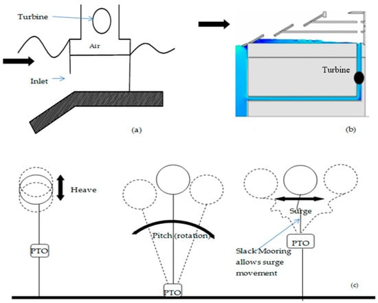
Figure 1.
Classification of wave energy converter (WEC) extraction technologies: (a) oscillating water column, (b) overtopping devices and (c) oscillating bodies [2].
One of the promising methods of wave energy capture is the oscillating body system. One major thing that makes the use of these types of converters attractive is because the amount of the energy absorbed by the body can be improved upon significantly under the same wave conditions when the body is at resonance with the incoming waves as illustrated in Figure 2. In fact, the team that won the prestigious ocean wave energy prize offered by the United States Department of Energy developed their concept and design based on a heavingf oscillating buoy [25]. The Pelamis [26], which is one of the most studied converters, is a pitching (rotating) oscillating converter and is also another type of a wave activated body system.
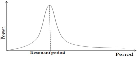
Figure 2.
Illustration of theoretical power capture of oscillating body system converters [1,2].
The hydrodynamics of oscillating body systems including heaving systems were independently solved by [27,28,29], which show the theoretical maximum energy to be captured by an oscillating body system-based wave energy converter. The results confirm that the highest possible capture occurs when the body is at resonance with the incoming waves. This behavior of a floating oscillating body poses a challenge for WEC designers because a typical body has a narrow resonance frequency band, and the body performs poorly outside this band. Hence, one of the many characteristics of a good oscillating WEC design is to make the buoy resonate to the prevailing ocean wave properties [2]. It should be noted that other factors, including survivability and profitability, need to be considered as well when designing a WEC. In order to capture considerable power outside the resonance frequency band, different optimization methods have been proposed and investigated. Some optimization methods include changes made to the shape and dimensions of the buoy [30], while latching and declutching methods [31] are also used in some existing studies. Latching control is achieved by holding the heaving WEC in a fixed position when the velocity is zero and releasing it at the right time so that its velocity can be in phase with the excitation force to achieve resonance [32]. On the other hand, declutching works by alternatively switching the power take off system on and off [31]. Another method is the model predictive control. It is an advanced control strategy [33] compared to the passive control methods, which may employ complex algorithms and simulations to achieve the optimization of power absorption by the WECs. While these methods have theoretical possibilities, there exists very little information reporting their applications in real ocean conditions.
In all these designs and optimization methods, the ocean wave properties have to be properly characterized first in order to have a good and effective WEC design. Although two ocean wave properties (wave height and wave period) guide the estimation of ocean wave resource potential and power capture of a WEC, it is the wave period that determines how the resonance behavior of a floating body will be engineered so it will operate near resonant level with the desired ocean wave period. There are existing studies that focus on general guidelines for designing a WEC. Meanwhile, most available wave condition database or monitoring/forecasting systems are designed for other marine systems instead of WEC design [8,9], so it is important to investigate the possibility of using existing wave condition data on designing a WEC. Instead of optimizing the size of a heaving point absorber WEC, this paper focuses on conducting detailed quantitative analysis on the changes on the power output of a heaving point absorber due to the variation of temporal and spatial resolutions of existing wave condition data. This paper uses available wave condition data from an existing database instead of collecting new wave condition data in the analysis. Section 2 introduces the methodology used including the ocean wave data analysis in the studied regions, the method for estimating the average yearly energy resource potential as well as the design process for the WEC which led to two different WEC designs in terms of dimensions. In Section 3, the annual energy resource potential is estimated under three different scenarios based on existing wave condition data: (1) wave data based on hourly resolution at the selected location in the Gulf of Mexico, (2) wave data based on daily resolution at the selected location in the Gulf of Mexico, and (3) wave data based on hourly resolution in an offshore location in Oregon. The power and annual energy matrices of the two WEC designs based on the hourly and daily resolution data are analyzed in Section 4. The design tailored to the hourly resolution data in the Gulf of Mexico is tested with the hourly data of an offshore location in Oregon, and the results are compared. Section 5 shows the results of a series of statistical hypothesis analysis such as t-test using data obtained from the Gulf of Mexico to determine the significance on the power output by different parameters such as diameter, design and seasonal variation (winter and summer). Section 6 is for discussions and conclusions.
2. Methods
2.1. Ocean Wave Data
Existing default data of significant wave height and dominant wave period over a 9-year period was obtained from a buoy operated by National Data Buoy Center at a location in the Gulf of Mexico (GoM) at coordinates 26.968° N and 96.693° W with sea depth of 84 m in a watch circle of radius 138 m (Figure 3a) [34]. The percentage of occurrences were analyzed for two scenarios in terms of the temporal variation of the collected data: data obtained hourly (Table 1) and data obtained daily (Table 2). The daily and hourly significant wave height data represent the average of the highest one-third of waves in the given period of capture. For both datasets, the wave heights ranged from 1 m to 5 m and wave periods ranging from 3 s to 12 s captured about 99% of all data points. Another set of ocean wave data was obtained from a location in Oregon which is close to the PacWave test site at coordinates 44.667° N and 124.515° W with sea depth of 140 m and a watch circle of radius of 230 m (Figure 3b) [34]. Another reason to choose the Oregon site for comparison is that the Oregon site is considered as high wave energy potential site (Table 3) while the GoM site is normally considered as low wave energy potential site. It should be noted that extreme wave conditions exist with a very small occurrence, such that there are 0.0001% of waves with significant wave height larger than 12 m and dominant wave period higher than 22 s in the GoM. However, we didn’t include these extreme wave conditions in the data tables and power generation estimation, because the focus of this paper is on the power generation, while the proposed WEC will not generate power during the extreme conditions. The extreme conditions will be considered when investigating the structural reliability of the proposed WEC.
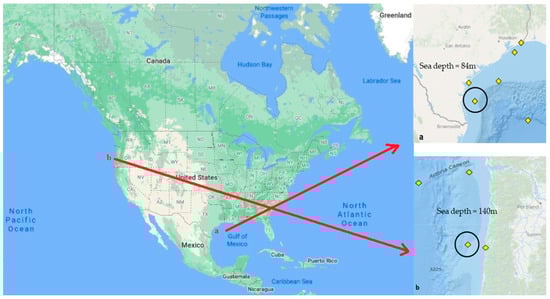
Figure 3.
Studying locations: (a) location 1: Gulf of Mexico, and (b) location 2: Oregon [34].

Table 1.
Percentage of ocean wave height and period occurrence based on hourly wave data (location 1: Gulf of Mexico).
Table 2.
Percentage of ocean wave height and period occurrence based on daily resolution data (location 1: Gulf of Mexico).
Table 3.
Percentage of ocean wave height and period occurrence based on hourly resolution data (location 2: Oregon).
2.2. Design of Heaving WEC Dimensions
The initial dimensions of the proposed WEC (Figure 4) were estimated based on the theoretical hydrodynamics of floating bodies. The hydrodynamics describe the motion of a floating body under the action of external forces. The external forces in this case were mainly generated by the ocean waves. A combination of wave data analysis and the theoretical wave hydrodynamics were used to estimate the diameter of the cylindrical buoy, which is the shape of the proposed WEC device. From the wave data analysis shown in Table 1 and Table 2, the dominant wave period falls between 5 and 6 s with 26.38% occurrence for the hourly data and between 6 and 7 s with 31.38% occurrence for the daily data. The following sets of equations were used to estimate the initial dimensions of the proposed WEC.
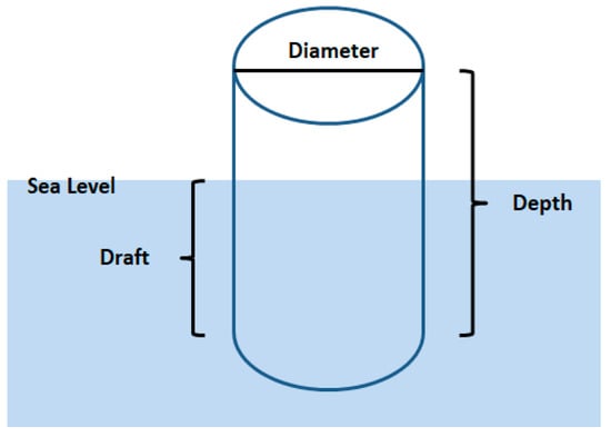
Figure 4.
Schematic design of the proposed WEC buoy.
From previous literature [35],
and as recommended by [36],
where Lmax is Maximum capture width, is wave length, T is dominant wave period, D is buoy diameter, C is captured width ratio and g is gravitational constant. These equations act as a guide to determine the size of a point absorber at the initial stage. It should be noted that Equation (2) is based on approximation made for deep water condition.
Theoretically, the resonance frequency of a submerged body is given by Equation (4) below. This simplified equation can be used at an initial stage to estimate the natural frequency of the point absorber system.
where Aw = water plane area, Mw
is mass of displaced water, a is added mass and
ωn is natural period. Added mass at this
preliminary stage is given as 0.167 ρD3 [36]. The effective drafts for different
diameters of a buoy whose density is equal to the density of water is given in
Table 4. This
application is for floating bodies alone. Steel is chosen as the material for
the buoy in this paper. For the buoy to oscillate freely in seawater, the buoy
must be hollow as the density of steel is greater than that of water. The mass
of the steel buoy should be equal to the mass of the displaced water such that
where, Ms is the mass of the steel cylindrical buoy.
Mw = Ms;
Table 4.
Dimensions of initial designs of the proposed WEC. GoM = Gulf of Mexico.
For any selected diameter and wave period, the corresponding draft and depth under 0.15 m thickness can be obtained in Table 5 and Table 6, respectively. It should be noted that the depth of the buoy (Table 6) must be greater than or equal to the draft (Table 5) for a floating cylinder. Thus, the feasible diameter of the buoy is 5 m and above. According to Equation (4), the resonance period is a function of mass of displaced water, water plain area, etc. Thus, for any thickness, the mass of water displaced and the mass of the cylindrical buoy should be constant when choosing the diameter of the buoy, but the depth of the cylinder will change. Therefore, the impact of the buoy thickness on its performance may be minimal in this research. For the initial design of the buoy in this paper, 8 m was chosen as its diameter with a steel of density 7850 kg/m3. For design 1, whose dimensions were tailored to the most probable wave period of the hourly resolution data in the GoM, the most prevalent wave period lies between 5 and 6 s, so the initial draft and depth of design 1 were 7.3 m and 12.9 m, respectively. Similarly, for design 2, whose dimensions were tailored to the most prevalent wave period between 6 and 7 s of the daily resolution data in the GoM, the initial draft and depth of design 2 were 10.5 m and 18.6 m, respectively. These initial dimensions were further analyzed in ANSYS diffraction module to give more accurate values of the resonance period corresponding to the initial dimensions, which decide the final dimensions used to estimate the power capture of the WEC.
Table 5.
Draft under different diameters and wave periods to achieve resonance (density of material = density of sea water).
Table 6.
Depth under different diameters and wave period to achieve resonance (density of material = density of steel).
A buoy diameter and associated draft used to form initial dimensions were tested using ANSYS/AQWA 18.1 [37]. ANSYS/AQWA is capable of simulating linearized hydrodynamic fluid wave loading on either floating or fixed rigid structures based on potential flow theory. It employs a three-dimensional diffraction theory in regular waves in the frequency domain. Furthermore, real time motion and force responses of bodies operating in regular or irregular waves can be studied. For each prevailing wave period based on the two temporal resolution data, the optimal dimensions (depth and draft to make buoy resonate with the wave period) for the selected diameters were decided after the analysis in ANSYS. AQWA The process is summarized in Figure 5.
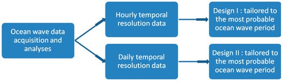
Figure 5.
Design process for arriving at each design.
3. Annual Energy Resource Assessment and Estimation
The ocean wave power density in a location is a function of wave height and wave period given by the relation in Equation (6) based on approximation made for deep water condition.
The annual power density can be estimated if information about the percentage occurrence of the wave height/period in the location is available [2].
where P (KW/m) is power density (power per unit width of wave front), ρ (Kg/m3) is seawater density, g (m/s2) is gravitational acceleration, H (m) is significant wave height and Te (s) is energy wave period. Since the wave period date provided by National Oceanic and Atmospheric Administration (NOAA) is dominant wave period Tp, the energy wave period (Te) is calculated by multiplying a wave period conversion factor α to dominant wave period (Tp). In this study, the wave conversion factor was considered as 0.9, which is the equivalent of JONSWAP software [38] and has been used in the past by different studies [9,20,38].
The potential energy density per year is calculated by multiplying the percentage occurrence in a year, and the results for the three different scenarios are provided in the Table 7, Table 8 and Table 9 below. From Table 7 and Table 8, the hourly resolution data provides annual energy density potential of 105.3 MWh/m, and the daily resolution data provides annual energy density potential of 102 MWh/m. This shows about 3% difference in terms of energy density potential in the same location with different temporal resolution data. This shows that different temporal resolution of the data in same location may not significantly affect the estimation of the total wave energy resource potential present in the location.
Table 7.
Annual energy density potential (kWh/(m∙yr)) based on hourly resolution data (location-1: Gulf of Mexico).
Table 8.
Annual energy density potential (kWh/(m∙yr)) based on daily resolution data (location-1: Gulf of Mexico).
Table 9.
Annual energy resource potential (kWh/(m∙yr)) based on daily resolution data (location-2: Oregon).
Similarly, the resource potential for the location in offshore Oregon is shown in Table 9 above. With a yearly total of about 43,374 MWhr/m of wave energy resource potential, it is confirmed that the location is a high wave energy resource area with resources about 40 times higher than that of the location in the Gulf of Mexico.
4. Power Capture of the WEC
Three scenarios of power capture are examined and compared in this section. After a series of computational fluid dynamics (CFD) diffraction analysis using ANSYS/AQWA suite version 18.1, which is based on potential flow theory, the response amplitude operator (RAO) which gives the motion response of the buoy at different periods is given in Figure 6. The three scenarios and the WEC dimensions are provided in Table 10. Design 1 was tailored to the dominant wave period based on the hourly resolution data while Design 2 dimensions was engineered to capture power optimally at the dominant wave period based on the daily resolution data from location 1 in the Gulf of Mexico. The power capture of design 1 in location 2 in Oregon is also estimated to investigate the impact of different wave conditions on the same WEC design in terms of power capture.
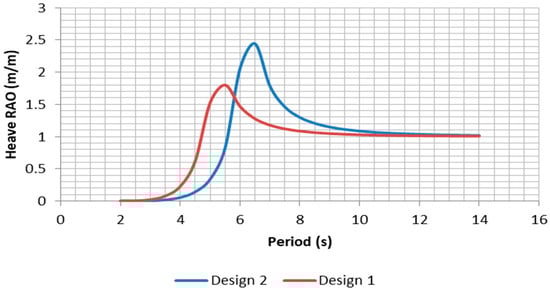
Figure 6.
Heave response amplitude for design 1 and design 2.
Table 10.
Dimension of the final designs used in three scenarios for estimating power capture. RAO = response amplitude operator.
The power take-off in this study was modeled as pure damper which is assumed to be frequency dependent. The motion equation of the heaving point absorber buoy with the power take off (PTO) can be described by Equation (7) below
where , M is mass, A is added mass, x is heave displacements and its derivatives with respect to time; B is damping coefficient and C is hydrostatic force coefficient; F(t) is the external force acting on the buoy while FPTO is the PTO force; and DPTO is the PTO damping coefficient.
The maximum amount of energy captured by the buoy occurs when the PTO damping is equal to the radiation damping of the buoy [39]. Hence the PTO damping will be equal to that of the buoy at resonance. The mean absorbed power by the PTO is given by Equation (8)
where, ω is the angular frequency at resonance.
Using the premises highlighted above, different values of PTO damping were tested on the buoy and the power capture and are shown in Figure 7. The maximum occurred when the damping coefficient was 50 kNm/s for both design 1 and design 2 when the diameter of the buoy was 8 m and 40 kNm/s when the diameter of the buoy was 7 m for both design scenarios.
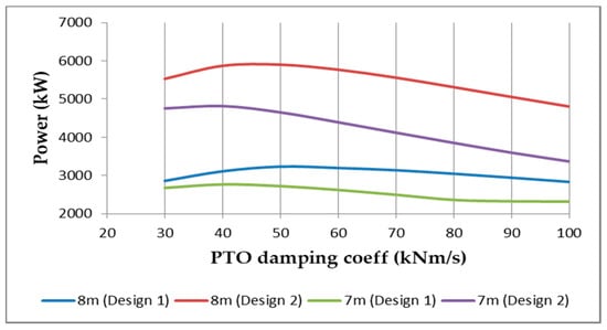
Figure 7.
Power take off (PTO) damping vs. power capture.
For both designs, the heaving oscillatory motion of the buoy was converted to power through a power take off (PTO). For the purpose of this design, a PTO damping of 40 kNm/s and 50 kNm/s was used for the WEC devices when the diameter of the buoy was 7 m and 8 m, respectively. Figure 8 and Figure 9 show the change of the power capture with respect to the wave period and wave height, respectively. The figures show, as expected, the power capture peaks when the wave period is at the resonance period of the buoy. However, the power capture increases almost linearly with wave height increase. Hence, while both wave period and wave height affect the power capture, the relationship between the wave period and power capture of a heaving point absorber is more significant due to the resonant behavior pattern.
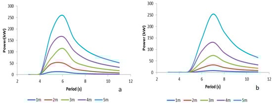
Figure 8.
Period vs. power: (a) hourly resolution power (b) daily resolution power.
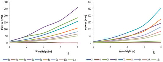
Figure 9.
Wave height vs. power: (a) hourly resolution power (b) daily resolution power.
The annual energy captured in each bivariate wave height-wave period combinations under different scenarios are given in Table 11, Table 12 and Table 13. Table 11 shows the yearly energy that can be harvested using design 1 tailored using the hourly data from the GoM, while Table 12 shows the comparative annual energy based on design 2 tailored using daily resolution data. Table 13 shows the annual energy by design 1 when operated in the Oregon location, an offshore region with over 40 times the wave energy potential compared to location 1 in the GoM. When the wave height-wave period combination did not exist due to physics of wave formation, “NA” is input in the tables, while a “0” in the table means the occurrence of that specific combination was zero in the specific time and location.
Table 11.
Annual energy matrix (Scenario-1: Gulf of Mexico).
Table 12.
Annual energy matrix (Scenario-2: Oregon).
Table 13.
Annual energy matrix (Scenario 3).
The result shows that the total annual energy capture under Scenario 1 was about 212 MWh/yr while Scenario 2 had about 178 MWh/yr. Scenario 3 had about 150 MWh/yr. The results show about 16% difference between Scenarios 1 and 2. It is also interesting to note that the annual energy performance estimation of design 2 was lower than that of that of design 1 even though the dimensions of design 2 were larger. It can be inferred that the temporal resolution of the ocean wave data also significantly affects the overall energy performance of the device in addition to significantly affecting the dimensions of the WEC buoy. When comparing Scenario 1 with Scenario 3, despite the buoys in both scenarios having the same dimensions, the total annual estimated energy capture in Scenario 1 was about 41% greater than that of the Scenario 3 even though the total annual energy theoretical potential in location 2 is over 40 times greater than that of location 1. This reinforces the idea that heaving buoys should be designed and tailored to specific locations. In the next section, the factors involved in the power capture estimation in this paper are further analyzed by conducting detailed statistical analysis.
5. Design Parameters and Their Effects on WEC’s Power Output
Different parameters and their effects on the WEC’s power production are tested using statistical hypothesis testing methods such as t-tests and factorial analysis. These tests have given more insights into the complexities that exist between some of different parameters that contribute to the energy produced by a WEC. Real ocean data of a 7-day period randomly picked from summer (July, 13–19) and winter (Jan, 1–7) in the GoM. One summer week and one winter week wave data are extracted including both hourly resolution (168 data points) and daily resolution (7 data points). The power output of WECs with different design parameters including design types (design 1& design 2) and diameters (7 m & 8 m) are estimated under the two weeks wave data. These estimated power output values are used as samples for the hypothesis testing. For the two-sample two-tailed t-test under hourly and daily data, each sample has 168 and 7 data points, respectively. For the factorial analysis, the estimated power output values are considered as the response/variable, and design type, diameter, and season are considered as factors with each factor having two different levels.
For the hourly resolution data within the week used for design 1, the standard deviations of the wave height and wave period are 0.32 m and 1.03 s for the summer and 0.65 m and 1.05 s for the winter. Similarly, for the daily resolution data used for design 2, the standard deviations of the wave height and wave period are 0.25 m and 0.69 s for the summer and 0.54 m and 0.78 s for the winter. As described in previous sections, design 1 is tailored to capture highest energy between 5–6 s (RAO = 5.5 s), and design 2 is tailored to capture most energy between 6–7 s (RAO = 6 s). So the distribution of wave period within the selected period does influence the results. For the winter season, the wave period falls below 6 s for 95 times out of 168 for the hourly resolution data and 4 times out of 7 times for the daily resolution data. Similarly for the summer season, the wave period falls below 6 s for 23 times for the hourly data and zero time for the daily data. The results of the two-sample two-tailed t-tests are shown in Table 14, where the estimated power outputs are the samples.
Table 14.
Results of Series of t-tests.
From the results, a p-value less than or equal to 5% indicates that the variables (parameters) significantly influenced the power output. First, different designs (design 1 versus design 2) significantly affected the power output irrespective of the season and diameter. Second, for the seasonal variations, most results were significant except for when the diameter was 7 m in design 2. Last, the size of the diameters in most cases significantly affected the power output of the device, except for design 1 during the winter time.
The factorial analysis was performed on the power output with design, diameter and season as the factors. Each factor had two different levels, so a 23 factorial design was formed and tested. The results from the factorial analysis are shown in Table 15. The results show a p-value of less than 5% for all the main effects and interaction between design and season, while the remaining two-way and three-way interactions were not significant.
Table 15.
Results (p-value) of the 23 factorial design analysis.
6. Conclusions
The effects of the spatial and temporal resolution of the ocean wave data on the design of heaving point absorber and its power capture have been analyzed in this study. The effects have been analyzed quantitatively by comparing power capture performance of different designs of heaving point absorber based on different temporal and spatial wave conditions. By applying the normal convention to design the WEC device to resonate, it would capture energy in the most prevalent ocean wave period. The results show that different temporal resolution data lead to different designs, which may capture different amount of energy. However, the difference in temporal resolution of data did not significantly affect the estimation of the ocean wave theoretical power present in a location.
The results confirm the importance of designing a WEC device specific to a location. The WEC device designed to operate in a region in the Gulf of Mexico may generate much less energy in an offshore location in Oregon, even though Oregon location has almost 40 times more ocean wave energy potential than the location in the Gulf of Mexico. Results of these analysis show that the power captured by the same device in the Gulf of Mexico was higher despite having lesser wave energy potential. This is because the WEC was designed to resonate with the prevalent ocean wave condition in the Gulf of Mexico, so its performance was poor in the Oregon location. The influence of the WEC design, diameter and seasonal changes were also examined on the power output of the device. These effects were analyzed using t-tests and factorial analysis. The results show that all the parameters to varying degrees have significant effect on the power output. However, only the interaction between design and season shows significant effect. Furthermore, a linear damper of 40 kNm/s and 50 kNm/s was used in this paper to represent the power take off for the 7 m and 8 m buoy. Future studies will perform sensitivity analysis to determine the optimal damper and its nonlinear behavior.
Studying the complexities that exists in the interaction of WEC devices with the ocean waves will increase the knowledge in the design of more effective devices, which will make the penetration of ocean wave energy increase. The scope of this study deals with only the primary capture of mechanical energy from the ocean waves through the hydrodynamic interaction of the WEC device and is most useful at the feasibility stage of the project. This aspect is only a part of the wave energy process, which includes the hydrodynamic conversion, conversion to electrical energy, and transmission. The wave condition data used in this paper was obtained from NOAA directly, which provides hourly and daily resolution. During the feasibility analysis stage of wave energy harvesting and WEC design, it was possible to directly use existing wave condition data with default temporal resolution as many existing studies did [4,6,8,40,41,42,43,44,45]. Meanwhile, IEC TC114 technical specification recommends 30 min temporal resolution when designing WECs for commercial use. Decision makers and WEC designers should choose the right temporal resolution based on different needs and budget limitations. As the commercialization of WECs draws more attention, it is expected more wave condition data with 30 min temporal resolution may become available, which could reduce the additional cost for collecting wave energy data for WEC designs. In addition, the structural reliability of any WEC devices should also be considered in the design stage, especially their reliability under extreme and hash ocean wave conditions.
Author Contributions
T.A. conducted data collection, product design and data analysis with the suggestions and guidance from H.L. T.A. wrote the initial draft paper under the supervision of H.L. H.L. made major revision on the initial draft paper, and approved the final version to be published. All authors have read and agreed to the published version of the manuscript.
Funding
This research received no external funding.
Acknowledgments
The authors are thankful to the support from Texas A&M University-Kingsville and National Science Foundation (award # EEC-1757812).
Conflicts of Interest
The authors declare no conflict of interest.
References
- Pecher, A.; Kofoed, J.P. Handbook of Ocean Wave Energy; Springer: London, UK, 2017. [Google Scholar]
- Aderinto, T.; Li, H. Ocean wave energy converters: Status and challenges. Energies 2018, 11, 1250. [Google Scholar] [CrossRef]
- Lehmann, M.; Karimpour, F.; Goudey, C.A.; Jacobson, P.T.; Alam, M.R. Ocean wave energy in the United States: Current status and future perspectives. Renew. Sustain. Energy Rev. 2017, 74, 1300–1313. [Google Scholar] [CrossRef]
- Reguero, B.G.; Losada, I.J.; Méndez, F.J. A global wave power resource and its seasonal, interannual and long-term variability. Appl. Energy 2015, 148, 366–380. [Google Scholar] [CrossRef]
- Izadparast, A.H.; Niedzwecki, J.M. Estimating the potential of ocean wave power resources. Ocean Eng. 2011, 38, 177–185. [Google Scholar] [CrossRef]
- Jacobson, P.T.; Hagerman, G.; Scott, G. Mapping and Assessment of the United States Ocean Wave Energy Resource; Electric Power Research Institute: Palo Alto, CA, USA, 2011. [Google Scholar]
- The Crown Estate. UK Wave and Tidal Key Resource Areas Project—Summary Report; WWW Document; The Crown Estate: London, UK, 2012. [Google Scholar]
- Haces-Fernandez, F.; Li, H.; Jin, K. Investigation into the possibility of extracting wave energy from the Texas coast. Int. J. Energy Clean Environ. 2019, 20, 23–41. [Google Scholar] [CrossRef]
- Fernandez, F.H.; Martinez, A.; Ramirez, D.; Li, H. Characterization of wave energy patterns in Gulf of Mexico. In Proceedings of the Institute of Industrial and Systems Engineers Annual Conference, Pittsburgh, PA, USA, 20–23 May 2017; pp. 1532–1537. [Google Scholar]
- Silva, D.; Bento, A.R.; Martinho, P.; Soares, C.G. High resolution local wave energy modelling in the Iberian Peninsula. Energy 2015, 91, 1099–1112. [Google Scholar] [CrossRef]
- Mentaschi, L.; Besio, G.; Cassola, F.; Mazzino, A. Performance evaluation of Wavewatch III in the Mediterranean Sea. Ocean Model. 2015, 90, 82–94. [Google Scholar] [CrossRef]
- Gallagher, S.; Tiron, R.; Whelan, E.; Gleeson, E.; Dias, F.; McGrath, R. The nearshore wind and wave energy potential of Ireland: A high resolution assessment of availability and accessibility. Renew. Energy 2016, 88, 494–516. [Google Scholar] [CrossRef]
- Liang, B.; Shao, Z.; Wu, G.; Shao, M.; Sun, J. New equations of wave energy assessment accounting for the water depth. Appl. Energy 2017, 188, 130–139. [Google Scholar] [CrossRef]
- Chen, X.; Wang, K.; Zhang, Z.; Zeng, Y.; Zhang, Y.; O’Driscoll, K. An assessment of wind and wave climate as potential sources of renewable energy in the nearshore Shenzhen coastal zone of the South China Sea. Energy 2017, 134, 789–801. [Google Scholar] [CrossRef]
- Seemanth, M.; Bhowmick, S.A.; Kumar, R.; Sharma, R. Sensitivity analysis of dissipation parameterizations in a third-generation spectral wave model, WAVEWATCH III for Indian Ocean. Ocean Eng. 2016, 124, 252–273. [Google Scholar] [CrossRef]
- Astariz, S.; Iglesias, G. The economics of wave energy: A review. Renew. Sustain. Energy Rev. 2015, 45, 397–408. [Google Scholar] [CrossRef]
- Witt, M.J.; Sheehan, E.V.; Bearhop, S.; Broderick, A.C.; Conley, D.C.; Cotterell, S.P.; Hosegood, P. Assessing wave energy effects on biodiversity: The Wave Hub experience. Philos. Trans. R. Soc. A 2012, 370, 502–529. [Google Scholar] [CrossRef] [PubMed]
- Elwood, D.; Yim, S.C.; Prudell, J.; Stillinger, C.; Von Jouanne, A.; Brekken, T.; Paasch, R. Design, construction, and ocean testing of a taut-moored dual-body wave energy converter with a linear generator power take-off. Renew. Energy 2010, 35, 348–354. [Google Scholar] [CrossRef]
- Babarit, A. A database of capture width ratio of wave energy converters. Renew. Energy 2015, 80, 610–628. [Google Scholar] [CrossRef]
- Haces-Fernandez, F.; Li, H.; Ramirez, D. Assessment of the potential of energy extracted from waves and wind to supply offshore oil platforms operating in the Gulf of Mexico. Energies 2018, 11, 1084. [Google Scholar] [CrossRef]
- Falnes, J.; Lillebekken, P.M. Budal’s latching-controlled-Buoy TypeWave-power plant. In Proceedings of the 5th European Wave Energy Conference, Cork, UK, 17–20 September 2003. [Google Scholar]
- Waveroller. Available online: http://aw-energy.com/aboutwaveroller/waveroller-concept (accessed on 30 May 2019).
- Al Shami, E.; Zhang, R.; Wang, X. Point absorber wave energy harvesters: A review of recent developments. Energies 2019, 12, 47. [Google Scholar] [CrossRef]
- EMEC. Pelamis Wave Power. Available online: http://www.emec.org.uk/about-us/wave-clients/pelamis-wave-power/ (accessed on 30 May 2019).
- Dallman, A.; Jenne, D.S.; Neary, V.; Driscoll, F.; Thresher, R.; Gunawan, B. Evaluation of performance metrics for the Wave Energy Prize converters tested at 1/20th scale. Renew. Sustain. Energy Rev. 2018, 98, 79–91. [Google Scholar] [CrossRef]
- Thomson, R.C.; Chick, J.P.; Harrison, G.P. An LCA of the Pelamis wave energy converter. Int. J. Life Cycle Assess. 2019, 24, 51–63. [Google Scholar] [CrossRef]
- Evans, D.V. A theory for wave-power absorption by oscillating bodies. J. Fluid Mech. 1976, 77, 1–25. [Google Scholar] [CrossRef]
- Evans, D.V.; Porter, R. Hydrodynamic characteristics of an oscillating water column device. Appl. Ocean Res. 1995, 17, 155–164. [Google Scholar] [CrossRef]
- Mei, C.C. Power extraction from water waves. J. Ship Res. 1976, 20, 63–66. [Google Scholar]
- Shadman, M.; Estefen, S.F.; Rodriguez, C.A.; Nogueira, I.C. A geometrical optimization method applied to a heaving point absorber wave energy converter. Renew. Energy 2018, 115, 533–546. [Google Scholar] [CrossRef]
- Wu, J.; Yao, Y.; Zhou, L.; Göteman, M. Latching and declutching control of the solo duck wave-energy converter with different load types. Energies 2017, 10, 2070. [Google Scholar] [CrossRef]
- Feng, Z.; Kerrigan, E.C. Latching control of wave energy converters using derivative-free optimization. In Proceedings of the 52nd IEEE Conference on Decision and Control, Florence, Italy, 10–13 December 2013; pp. 7474–7479. [Google Scholar]
- Li, G.; Belmont, M.R. Model predictive control of sea wave energy converters–Part I: A convex approach for the case of a single device. Renew. Energy 2014, 69, 453–463. [Google Scholar] [CrossRef]
- National Data Buoy Center. Available online: https://www.ndbc.noaa.gov/ (accessed on 30 May 2019).
- Budar, K.; Falnes, J. A resonant point absorber of ocean-wave power. Nature 1975, 256, 478. [Google Scholar] [CrossRef]
- Hooft, J.P. Oscillatory wave forces on small bodies. Int. Shipbuild. Prog. 1970, 17, 127–135. [Google Scholar] [CrossRef]
- ANSYS AQWA, version v18.1; ANSYS Inc.: Canonsburg, PA, USA, 2018.
- Haces-Fernandez, F.; Li, H.; Ramirez, D. Wave energy characterization and assessment in the US Gulf of Mexico, East and West Coasts with Energy Event concept. Renew. Energy 2018, 123, 312–322. [Google Scholar] [CrossRef]
- Falnes, J.; Perlin, M. Ocean waves and oscillating systems: Linear interactions including wave-energy extraction. Appl. Mech. Rev. 2003, 56, B3. [Google Scholar] [CrossRef]
- Gunn, K.; Stock-Williams, C. Quantifying the global wave power resource. Renew. Energy 2012, 44, 296–304. [Google Scholar] [CrossRef]
- Ahn, S.; Haas, K.A.; Neary, V.S. Wave energy resource classification system for US coastal waters. Renew. Sustain. Energy Rev. 2019, 104, 54–68. [Google Scholar] [CrossRef]
- Robertson, B.; Hiles, C.; Luczko, E.; Buckham, B. Quantifying wave power and wave energy converter array production potential. Int. J. Mar. Energy 2016, 14, 143–160. [Google Scholar] [CrossRef]
- Ferrari, F.; Besio, G.; Cassola, F.; Mazzino, A. Optimized wind and wave energy resource assessment and offshore exploitability in the Mediterranean Sea. Energy 2019, 190, 116447. [Google Scholar] [CrossRef]
- Allahdadi, M.N.; Gunawan, B.; Lai, J.; He, R.; Neary, V.S. Development and validation of a regional-scale high-resolution unstructured model for wave energy resource characterization along the US East Coast. Renew. Energy 2019, 136, 500–511. [Google Scholar] [CrossRef]
- Yang, Z.; Neary, V.S.; Wang, T.; Gunawan, B.; Dallman, A.R.; Wu, W.C. A wave model test bed study for wave energy resource characterization. Renew. Energy 2017, 114, 132–144. [Google Scholar] [CrossRef]
Publisher’s Note: MDPI stays neutral with regard to jurisdictional claims in published maps and institutional affiliations. |
© 2020 by the authors. Licensee MDPI, Basel, Switzerland. This article is an open access article distributed under the terms and conditions of the Creative Commons Attribution (CC BY) license (http://creativecommons.org/licenses/by/4.0/).