The Heterogenous Demand for Urban Parks between Home Buyers and Renters: Evidence from Beijing

Abstract

Many studies have confirmed that there is demand among urban residents and renters for urban parks. Moreover, as renters and home buyers have very different levels of ownership over their housing resources, their demands for amenities can be heterogenous. To discover and identify such heterogeneous demands is worthy of attention. Using the micro-housing resale transactions and listing data for housing leases in Beijing during 2019, this paper explores the difference between the demand for urban parks among home buyers and renters outside the community from the perspective of the internal quality of the community by using the hedonic price model (HPM). Specifically, from the dimension of the property management service fee and greening rate, we find that for home buyers, compared to residents living in relatively poor-quality communities, a better-quality community will reduce the demand for urban parks outside the community. Conversely, for renters, the higher the quality of the community is, the higher the demand for urban parks outside the community will be.

1. Introduction

Realizing the seriousness of the climate change consequences in an urban context, people have begun to attach importance to urban ecosystem functions. Therefore, mitigation and adaptation should be used to maintain the provisions of ecosystem services [1]. As an important part of urban green space, urban parks play an important role in reducing the impact of climate change, especially in urban heat islands [2]. Therefore, estimating the demands of urban residents for urban parks is essential to better identify and understand the benefits of urban parks and promote both demand-oriented planning and the sustainable development of urban parks through market-oriented and more efficient supply.

Using the hedonic price model (HPM), many scholars have identified residents’ willingness to pay for local public goods (such as medical care, education, transportation, and urban parks) through the capitalization effect of local public goods on the housing sales market [3,4,5,6]. Compared to the abundant research on the capitalization effect of green space on housing prices, a small amount of research also confirms the positive impact of green spaces on rent [7,8]. Previous research on the demand for urban parks only confirms that residents have a strong demand for urban parks [9,10,11,12,13]. However, few studies take into account the heterogeneous demands of different residents—that is, the different demands of home buyers (home is a mixture which includes houses, apartments, and flats) and renters for urban parks, which need greater consideration [14].

Home buyers and renters differ greatly in their demands for surrounding public goods [15,16,17]. From a traditional perspective, home buyers enjoy the ownership of their house with a series of additional resources [18]. Therefore, the price that people pay when buying a house also includes the willingness to pay for public goods other than the house itself [19]. As housing prices involve speculation about future capital gains, including investments in surrounding public transport facilities and environmental improvements, using housing price data for evaluation may overestimate the premium yielded by the surrounding public goods [12,20,21]. On the other hand, rent shows the renter’s willingness to pay for the current public goods surrounding the house. Different demands for housing have led renters and home buyers to pay different levels of attention to various factors when conducting housing leasing or buying transactions [14,22]. Home buyers value medical and educational resources, while renters pay more attention to the convenience of transportation and living facilities, such as small convenience stores and vegetable markets, rather than large shopping malls [23,24]. In short, the consumption behavior of renters is stronger, and changes in rent reflect the renter’s living needs, while housing prices reflect the various demands of residents to buy a house. If only the demand of home buyers for urban parks is analyzed, the results cannot fully reflect the demands of the majority of residents in the real estate market (the real estate market includes the housing sales market and the rental market in this paper) [21,22,23,24]. Therefore, accurate identification and understanding of the differences between home buyers and renters in their demand for urban parks is important for the planning and sustainable development of urban parks. To better understand the heterogenous demand for urban parks between home buyers and renters, it is worthwhile to conduct empirical studies based on data covering a longer duration and with enough diversified housing transaction information.

For this reason, the city of Beijing would be a perfect study object considering its diversification of both urban residents and real estate market. Beijing’s real estate market provides a good opportunity to identify the heterogenous demands of home buyers and renters [25,26,27,28]. As the capital city of China, Beijing has excellent public service resources [20], such as employment, medical care, and education, that attract many non-local populations, who account for more than one third of Beijing’s total population. However, this resource attraction alongside the traditional housing consumption culture among Chinese residents has also led to extremely high house price premiums and a relatively cold residential rental market with a lack of cultivation and management [29]. To curb housing prices and stabilize the entire real estate market, the Chinese government focuses on the principles of a “house is for living in, not speculation”, and most Chinese cities, including Beijing, have gradually implemented policy interventions such as home purchasing restrictions and equal rights for home tenants and owners [30,31]. Equal rights for home tenants and owners and other policies promote the development of the residential rental market. The rental population in China’s service rental market has maintained steady growth since 2017, reaching 210 million in 2018. Driven by the pressure of buying houses and the development of the rental market, the sense of identity among house renters is increasing. Renting houses has become the new normal for young people in megacities, and most renters are under the age of 35, among which 21–25-year-olds account for one third of the total. This phenomenon reveals that young people no longer choose to buy a house prematurely but prefer to rent a house. The ages of first-time home buyers are also increasing. In Beijing, the average age of first-time home buyers increased from 26 in 2008 to 32 in 2018 (data source: the real estate data research platform “Beike Research Institute”, https://research.ke.com/). The rapid development of the rental market prevents us from neglecting the demands of renters.

Therefore, the purpose of this study is to explore the heterogeneous demands of home buyers and renters for urban parks considering different community traits through the HPM using the housing resale transaction data and listing housing lease data for 2019 from Beijing’s housing transaction website (the housing resale transactions in Beijing from 2011 to 2019 are about 1.62 million units, calculated based on the data from “Beijing Municipal Commission of Housing and Urban-Rural Development”). The remainder of the article is organized as follows. In the second section, we introduce the real estate market of Beijing in detail. The conceptual framework and research data are provided in the third section. The empirical results and analyses are presented in the fourth section, and the fifth section provides the discussion and conclusions.

2. Real Estate Market in Beijing

2.1. Features of Real Estate Market in Beijing

As China’s political, cultural, international communication, and science and technology innovation center, Beijing’s economic strength and superior resources have attracted a large number of mobile populations. At the end of 2019, the urbanization rate of Beijing reached 86.6%, with a permanent population of 21.536 million and a mobile population of 7.943 million, which accounts for 45.24% of the total population (data source: “Statistical Bulletin on the National Economy and Social Development of Beijing in 2019”). The real estate market is closely related to the livelihood of residents. A healthy real estate market can ease social conflicts and stabilize regional economies [31]. However, the development of Beijing’s real estate market is not balanced. Specifically, the housing sales market is booming, whereas the housing rental market is relatively deserted. The data show that the average price of housing resale transactions in Beijing in 2019 was 63,052 CNY/m² (data source: “Housing Prices of 320 Cities 2019”, https://www.chinadatapay.com/), ranking second in China, while the average rent in Beijing in March 2020 was 81.68 CNY/m²/month. The average house price–rent ratio in Beijing is over 700:1, well above the reasonable international range level of 200:1–300:1, which means that housing prices in Beijing are seriously overestimated [26]. According to previous research, due to the household registration (hukou) system [27], the scarcity of various resources (such as quality education and health care) available after purchasing a house has led to rising housing prices in Beijing, which caused and continues to aggravate the uneven development of the housing sales market and the rental market. Therefore, this policy makes it difficult for foreigners to buy and rent houses in Beijing [14]. In this context, it may be very important to have green resources (green resources in the urban context include urban parks, community greening, and forest landscapes) to enjoy at one’s place of residence.

Buying and renting have their own advantages and disadvantages, and the choice between the two reflects the different preferences of buyers and renters. Compared to purchased housing, despite the lack of some specific resources, renting is a more flexible, convenient, and affordable housing option. Individuals can choose their optimal place of residence according to their own location preferences, location of employment, and payment ability, as well as minimize the cost of commuting [32].

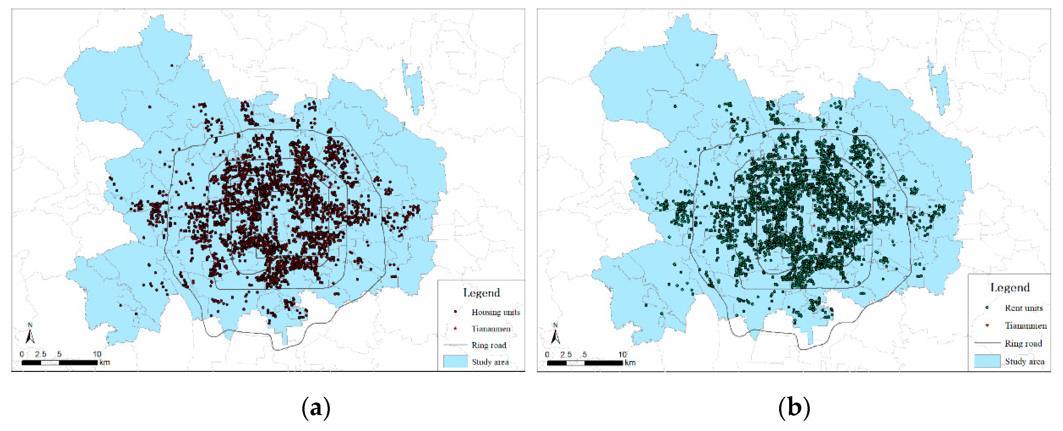
2.2. Distribution of Housing in our Study Area

Our study area includes the six districts (Dongcheng, Xicheng, Chaoyang, Haidian, Fengtai, and Shijingshan) of Beijing. The distribution of housing communities and rental communities in the study area is analogous (Figure 1). The spatial distribution characteristics are such that the phenomena of agglomeration and dispersion exist at the same time, which manifests as the obvious phenomenon of agglomeration in the central urban area. The spatial distribution of housing in Beijing presents the following characteristics: first, there are more houses in the north of Beijing than in the south, and second, there are more houses in the east than in the west. Judging from the distribution of housing estates, Chaoyang, Haidian, and Fengtai contain most of the city’s communities. The distribution density of residential districts in Dongcheng and Xicheng is much higher than that in other districts— that is, the degree of housing concentration in these two districts is high. For the ring road (ring road refers to the eight existing and planned ring highways in Beijing), the distribution density of the second ring to the third ring cell is the highest.

Within our study area, there were 32,884 housing resale transactions distributed among 2894 communities (as shown in Figure 1a) and 48,581 rental listing data distributed among 3069 communities (as shown in Figure 1b). As shown in Figure 1, most of the housing communities are located within the fifth ring road of Beijing.

3. Materials and Methods

3.1. Conceptual Framework

In this study, we adopt the commonly used HPM to measure the demands of home buyers and renters for factors and characteristics that have an impact on housing prices, which include the internal characteristics of the property itself (e.g., its size, appearance, and condition), community characteristics (e.g., if the neighborhood has a high greening rate), and location characteristics, particularly amenities (e.g., if the neighborhood is accessible to schools, hospitals, and subway stations). Our basic unit or sample of empirical analysis is a residential property p or rental property i in a community j that was transacted in month t, and our study period is 2019.

The semi-logarithmic form of the HPM for housing prices is shown in Equation (1), and the HPM for rent is shown in Equation (2):

$${\mathit{LnP}}_{p,t}{=\alpha }_0{+\alpha }_{11}{X}_{h,p}{+\alpha }_{12}{X}_{c,j}{+\alpha }_{13}{X}_{a,j}{+\alpha }_{14}{X}_{g,j}{+\phi }_t{+\phi }_s{+\epsilon }_{p,t}$$

(1)

$${\mathit{LnR}}_{i,t}{=\alpha }_0{+\alpha }_{21}{X}_{h,i}{+\alpha }_{22}{X}_{c,j}{+\alpha }_{23}{X}_{a,j}{+\alpha }_{24}{X}_{g,j}{+\phi }_t{+\phi }_s{+\epsilon }_{i,t}$$

(2)

where ${\mathit{LnP}}_{p,t}$ is the natural logarithm of housing prices for housing unit p, and ${\mathit{LnP}}_{i,t}$ is the natural logarithm of rent for housing unit i. In the above two equations, α₀ is the constant term, and ${\epsilon }_{p,t}$ and ${\epsilon }_{i,t}$ are the error terms. X_h,p/X_h,i is the physical characteristics of the housing unit p/i, X_c,j is the community characteristics of the community j, X_a,j represents the other amenities besides the urban parks of the community j, and X_g,j is the accessibility to parks for the community j. The coefficients of ${\alpha }_{11}$, ${\alpha }_{12}$, ${\alpha }_{13}$, and ${\alpha }_{14}$ to be estimated represent the contributions of X_h,p, X_c,j, X_a,j, and X_g,j to housing prices, and the coefficients of ${\alpha }_{21}$, ${\alpha }_{22}$, ${\alpha }_{23}$, and ${\alpha }_{24}$ to be estimated represent the contributions of X_h,i, X_c,j, X_a,j, and X_g,j to rent. ${\phi }_t$ controls for year-fixed effects, and ${\phi }_s$ captures jiedao-fixed effects (jiedao is the sub-district and basic administrative management unit of China). We introduce a combination of both spatial and temporal fixed effects into the HPM to deal with potentially missing variables [3]. The spatial fixed effect in this paper is controlled for each jidao, which is a basic administrative management unit of Beijing. There are 101 jiedaos in our study area, with an average area of 13.7 km² and an average population of 113,753 people (calculated based on the number of jiedao, the population, and the total area of our study area in Beijing). The temporal fixed effect for each month captures the potential changes in housing prices and rent over time in 2019.

To identify the heterogeneous demand for urban parks among homebuyers and renters caused by divergent community traits, we classify communities according to their property management service fee levels and greening rate (the green rate is calculated by the ratio of green land area to total area) levels and perform group regression based on Equations (1) and (2). If the property management (PM) fee of the community is lower than the median of all samples, it is marked as PM = 0. Otherwise, it is marked as PM = 1. By controlling other features, we introduce an interaction term of the park variable and the property management service fee variable (PM × Park) for housing price in Equation (3) and rent in Equation (4) to identify whether home buyer and renter demands for the park will be affected by the level of property management service fees in the community. Thus, the coefficient ${\alpha }_{13}$ represents the demand for parks among home buyers under the influence of relatively high property management service fees compared to communities with relatively low property management service fees, and the coefficients of ${\alpha }_{23}$ characterize the demand for parks among renters under the influence of relatively high property management service fees compared to communities with relatively low property management service fees. If the estimated coefficients of the interaction term in Equations (2) and (3) are significantly positive, we can infer that the demand of residents in communities with high property management service fees is higher than the demand in areas with low property management service fees, and vice versa.

$${\mathit{LnPPM}}_{p,t}{=\alpha }_0{+\alpha }_{11}{\mathit{Park}+\alpha }_{12}{\mathit{PM}+\alpha }_{13}{\mathit{PM}\times \mathit{Park}+\alpha }_{14}{X}_{a,j}{+\alpha }_i{X}_p{+\phi }_t{+\phi }_s{+\epsilon }_{p,t}$$

(3)

$${\mathit{LnRPM}}_{I,t}{=\alpha }_0{+\alpha }_{21}{\mathit{Park}+\alpha }_{22}{\mathit{PM}+\alpha }_{23}{\mathit{PM}\times \mathit{Park}+\alpha }_{24}{X}_{a,j}{+\alpha }_i{X}_i{+\phi }_t{+\phi }_s{+\epsilon }_{p,t}$$

(4)

Based on different greening rates, we divide the community sample into two sub-sample groups: a relatively high greening rate community and a relatively low greening rate community. If the greening rate of a community is higher than the median greening rate of the community sample, it will be marked as a relatively high greening rate community (Green = 1). If the greening rate of a community is lower than the median greening rate of the community sample, it will be marked as a relatively low greening rate community (Green = 0). We also introduce an interaction term of the park variable and the greening rate variable (Green × Park) for housing price in Equation (5) and rent in Equation (6) to analyze the difference between the demands of home buyers and renters for urban parks with high and low greening rates. The coefficients of ${\alpha }_{13}$ in Equation (5) and ${\alpha }_{23}$ in Equation (6) characterize the demand for parks among home buyers and renters under the influence of a relatively high greening rate compared to communities with a relatively low greening rate, respectively. If the estimated coefficients of the interaction term in Equations (2) and (3) are significantly positive, then the demand of the residents in communities with a high greening rate is higher than the demand in areas with a low greening rate, and vice versa.

$${\mathit{LnpGreen}}_{p,t}{=\alpha }_0{+\alpha }_{11}{\mathit{Park}+\alpha }_{12}{\mathit{Green}+\alpha }_{13}{\mathit{Green}\times \mathit{Park}+\alpha }_{14}{X}_{a,j}{+\alpha }_i{X}_p{+\phi }_t{+\phi }_s{+\epsilon }_{p,t}$$

(5)

$$\mathit{Ln}I{=\alpha }_0{+\alpha }_{21}{\mathit{Park}+\alpha }_{22}{\mathit{Green}+\alpha }_{23}{\mathit{Green}\times \mathit{Park}+\alpha }_{24}{X}_{a,j}{+\alpha }_i{X}_i{+\phi }_t{+\phi }_s{+\epsilon }_{p,t}$$

(6)

3.2. Definition of Variables and Basic Descriptive Statistics

Our dataset includes the physical characteristics of each house, the basic information of the community, GIS-based amenity variables, and accessibility from a community to nearby urban parks.

First, for the physical characteristics of each house, we apply seven variables: floor area (Area), age (Age), number of bedrooms (Bedroom) and living rooms (Livingroom), orientation status (Orient), floor (Floor), and degree of decoration (Decoration). Second, for the characteristics of the community in which the house is located, we consider five main variables: property management costs (Property costs), which represent the quality of community property management services and thus may reflect the quality of the community (we expect the estimated coefficient of this variable to be positive). We also consider the plot ratio (Plot ratio) and greening rate (Green rate), which, respectively, reflect the level of living comfort and greening conditions in a community. Lastly, for the locational amenities of a community besides accessibility to urban parks, we apply five variables: distance to the city center “Tiananmen Square”, which is also the employment center of Beijing (Dis_tam); distance to the to the nearest city employment sub-center of Zhongguancun, Wangjing, Guomao, Yayuncun, Jinrongjie, Shangdi, and Yizhuang (Dis_job); in a metropolis like Beijing, the convenience of the subway makes many people prefer the subway, so the influence of subway stations is wider than that of schools and hospitals. Therefore, we choose the number of subway stations within 1000 m of the community (Subway); and the presence of top-quality hospitals (Hospital) and key primary schools (Education) within 500 m of the community to represent the level of the location amenities. Locational amenities reflect the accessibility to different types of public service facilities around residential communities, which residents have a positive demand for. Detailed definitions and descriptive statistics of the variables are presented in

Table 1. Variable definitions and descriptive statistics.

Variable	Definition	Housing Price		Rent
		Mean	SD	Mean	SD
LnPrice/LnRent	Natural logarithm of housing price/rent	11.133	0.288	4.774	0.324
Physical Characteristics of Housing		N = 32884		N = 48581
Area	Total floor area of the house (m2)	79.513	36.178	65.947	38.794
Age	The age of the house (year)	22.670	10.418	24.147	12.009
Bedroom	Number of bedrooms in the house	2.019	0.744	2.095	0.934
Livingroom	Number of living rooms in a house	1.088	0.414	0.844	0.535
Orient_a	Orientation of a house, a series of dummy variables, a = [east, south, west, north, northeast, southeast, northwest, southwest], yes is 1, no is 0	-	-	-	-
Floor_a	Floor of the house, a series of dummy variables, a = [basement, ground floor, low floor, middle floor, high floor, top floor], yes is 1, no is 0	-	-	-	-
Decoration_a	The decoration status of the house, a series of dummy variables, a = [rough, sample, luxury, other], yes is 1, no is 0	-	-	-	-
Community Characteristics		N = 2894		N = 3069
Property costs	Property management service fees (CNY/month/m2)	1.899	1.429	2.125752	1.610
PM	Dummy variable, 1 = community with high property management service fees, 0 = otherwise	0.453	0.498	0.489	0.500
Green rate	The greening rate of the community	0.314	0.071	0.311	0.075
Green	Dummy variable, 1 = community with high greening rate, 0 = otherwise	0.865	0.341	0.844	0.363
Plot ratio	The ratio of the building floor area to the land area in a given territory	2.468	1.327	2.664	1.276
Park Accessibility		N = 2894		N = 3069
Dis_park	The distance from the community to the nearest park (m)	0.805	0.427	0.791	0.420
Park	Dummy variable, whether there is a park within 500 m of the community, yes is 1; no is 0.	0.132	0.340	0.307	0.461
Other Locational Amenities		N = 2894		N = 3069
Dis_tam	The distance from the community to the city center, Tiananmen Square (km)	9.308	3.982	8.864	3.872
Dis_job	The distance from the community to the nearest city employment sub-center (km): Zhongguancun, Wangjing, Guomao, Yayuncun, Jinrongjie, Shangdi, Yizhuang	5.296	3.398	4.773	3.193
Subway	Number of subway stations within 1000 m of the community	0.772	0.420	0.112	0.316
Education	Whether there is a key elementary school within 500 m of the community: yes is 1, no is 0	0.091	0.288	0.059	0.235
Hospital	Whether there is a top-quality hospital within 500 m of the community: yes is 1, no is 0	0.06	0.24	1.199	0.637

.

For the park variables, we measure the accessibility from a community to urban parks in two ways. On the one hand, a dummy variable is used to determine whether a park exists in the community within 500 m (Park). We expect that these variables will be significantly positive, reflecting urban residents’ strong demands. On the other hand, we also calculate the straight-line distance from a community to its nearest urban park (Dis_park).

3.3. Descriptive Statistics of the Park Accessibility in the Housing Samples and Rent Samples

Further, by grouping the greening rate and park accessibility according to the median of the housing samples and rent samples, we identified the differences in the internal greening rate and accessibility of external parks between the housing and rent samples (shown in

Table 2. The difference in internal greening rate and accessibility of external parks between the housing and rent samples.

	Dis_Park	Housing Samples		Rent Samples
Greening Rate		0–800 m	Greater Than 800 m	0–800 m	Greater Than 800 m
0–30%		0.289	0.272	0.316	0.259
Greater than 30%		0.224	0.215	0.218	0.206

). The median of Dis_park is 800 m, and the median of the greening rate in the community is 30%. In both the housing samples and the rent samples, the samples with a lower internal greening rate (Greening rate lower than 30%) and better external park accessibility (Dis_park lower than 800 m) account for the largest proportion, while the samples with the higher internal greening rate level (Greening rate higher than 30%) and higher external park accessibility (Dis_park lower than 800 m) account for the smallest proportion. Based on a comparison of the greening rate within the community, the proportion of communities with a high greening rate (Greening rate higher than 30%) in the samples of those buying a house is greater than that in the samples of those renting a house. From the comparison of the accessibility of parks, the proportion of communities with good park accessibility (Dis_park lower than 800 m) in the samples of those renting a house is greater than that in the samples of those buying a house.

From the perspective of property management service fees, we compare the difference between the community’s internal property management service fees and external park accessibility (as shown in

Table 3. The differences in internal property management service fees and the accessibility to external parks between the housing and rent samples.

	Dis_Park	Housing Samples		Rent Samples
PM Fee		0–800 m	Greater Than 800 m	0–800 m	Greater Than 800 m
0–1.65		0.280	0.237	0.267	0.223
Greater than 1.65		0.228	0.255	0.259	0.251

). Judging from the comparison results, the proportion of houses with lower property management service fees and better park accessibility accounts for the largest proportion in both the buying samples and the renting samples. Based on a comparison of the property management service fees in the community, the proportion of communities with high property management service fees (property management service fees greater than 1.65 CNY/m²/month) in the samples of those buying a house is greater than that among the renting samples. The accessibility to parks among the renting samples is also better than that of the housing samples.

4. Empirical Results

In this section, we introduce the main empirical findings of this paper from the following three perspectives. First, we compare the differences between home buyers and renters in their demands for various features and amenities, especially urban parks. Then, the community property management service fees and greening rates are used to characterize the two dimensions of community quality. The second part and the third part, respectively, compare the heterogeneous demands of residents and renters for urban parks with the two dimensions of the property management service fee and the greening rate.

4.1. Overall Different Demands between Homebuyers and Renters

The regression results of the HPM based on time and spatial fixed effects are shown in

Table 4. Housing price and rent hedonic regressions.

	Ln_Price			Ln_Rent
	(1)	(2)	(3)	(4)	(5)	(6)
Dis_Park			−0.0253 ***			−0.0220 ***
			(−10.665)			(−8.239)
Age	−0.0033 ***	−0.0074 ***	−0.0074 ***	−0.0028 ***	−0.0118 ***	−0.0119 ***
	(−22.635)	(−19.415)	(−19.496)	(−22.526)	(−27.798)	(−27.969)
Age2		0.0001 ***	0.0001 ***		0.0002 ***	0.0002 ***
		(13.552)	(13.464)		(23.243)	(23.418)
Area	−0.0015 ***	−0.0016 ***	−0.0016 ***	−0.0034 ***	−0.0035 ***	−0.0035 ***
	(−23.854)	(−25.055)	(−25.191)	(−35.748)	(−36.721)	(−36.952)
Bedroom	0.0202 ***	0.0218 ***	0.0221 ***	0.0595 ***	0.0603 ***	0.0603 ***
	(9.716)	(10.475)	(10.589)	(37.265)	(38.051)	(38.084)
Livingroom	0.0413 ***	0.0417 ***	0.0416 ***	−0.0385 ***	−0.0346 ***	−0.0347 ***
	(14.936)	(15.133)	(15.159)	(−12.076)	(−11.018)	(−11.078)
Propertycosts	0.0229 ***	0.0411 ***	0.0407 ***	0.0463 ***	0.0563 ***	0.0564 ***
	(19.783)	(24.772)	(24.578)	(45.113)	(29.945)	(30.003)
Propertycosts2		−0.0022 ***	−0.0022 ***		−0.0014 ***	−0.0013 ***
		(−12.892)	(−12.828)		(−7.504)	(−7.402)
Plotratio	−0.0170 ***	−0.0175 ***	−0.0174 ***	−0.0032 ***	−0.0042 ***	−0.0041 ***
	(−21.016)	(−21.777)	(−21.765)	(−3.997)	(−5.289)	(−5.201)
Greenrate	0.0168 ***	0.0174 ***	0.0170 ***	0.0191 ***	0.0189 ***	0.0185 ***
	(1.666)	(1.721)	(1.678)	(1.354)	(1.354)	(1.317)
Dis_tam	−0.0328 ***	−0.0170 ***	−0.0172 ***	−0.0237 ***	−0.0274 ***	−0.0240 ***
	(−28.388)	(−5.497)	(−5.534)	(−20.963)	(−8.258)	(−7.209)
Dis_job	−0.0012 ***	−0.0012 ***	−0.0013 ***	−0.0129 ***	−0.0131 ***	−0.0134 ***
	(−4.134)	(−4.175)	(−4.451)	(−13.034)	(−13.190)	(−13.496)
Subway	0.0400 ***	0.0404 ***	0.0417 ***	0.0621 ***	0.0610 ***	0.0609 ***
	(16.276)	(16.607)	(17.029)	(22.700)	(22.442)	(22.411)
Education	0.018 ***	0.020 ***	0.020 ***	0.0207 ***	0.0184 ***	0.0191 ***
	(7.531)	(8.372)	(8.982)	(7.208)	(6.448)	(6.667)
Hospital	0.0146 ***	0.0171 ***	0.0181 ***	0.0435 ***	0.0501 ***	0.0492 ***
	(3.848)	(4.577)	(4.859)	(9.548)	(10.952)	(10.827)
Constant	11.1397 ***	11.0731 ***	11.1122 ***	4.648 ***	4.727 ***	4.735 ***
	(442.141)	(374.400)	(356.278)	(244.539)	(180.690)	(166.449)
Year-fixed effect	Yes	Yes	Yes	Yes	Yes	Yes
Jiedao-fixed effect	Yes	Yes	Yes	Yes	Yes	Yes
N	32884	32884	32884	48581	48581	48581
R2	0.758	0.763	0.764	0.641	0.647	0.647

Note: (1) as there are too many variables, this table reports only the most important variables in this study. (2) *** p < 0.01. (3) The numbers in parentheses represent the robust t-statistics.

, with robust t-statistics in parentheses. Among them, the dependent variable in columns (1)-(3) is the housing price, and the dependent variable in columns (4) and (5) is rent. Both the HPM for housing price and the HPM for rent are controlled by variables of the physical characteristics of housing, community characteristics, and other location amenities. We also introduce “Dis_park” as the key variable for identifying the demand for urban parks in column (3) and column (6). The R² in the HPM for housing price is about 0.76, and that in the HPM for rent is about 0.65, indicating that our model can explain about 76% of the spatial variation in housing prices and 65% of the spatial variation in rent. Overall, the empirical results of the main control variables are in line with expectations.

According to the HPM for housing prices in column (1), among the physical characteristics of housing, variables such as “Age”, “Area”, “Bedroom”, “Livingroom”, “Propertycosts”, “Plotratio”, and “Greenrate” have significant effects on housing prices. Among them, the “Age” and “Area” coefficients are estimated to have negative signs, and “Bedroom” and “Livingroom” coefficients are estimated to be positive. Home buyers prefer new houses with smaller areas and more rooms and living rooms. The plot ratio and green rate reflect the building density and greening of the community, respectively. The plot ratio coefficient is estimated to be −0.0170, and the coefficient of the green rate is estimated to be 0.0168—that is, the higher the plot ratio of the community is, the lower the housing price will be. Conversely, the higher the green rate of the community is, the higher the housing price will be, indicating that residents prefer low building density and residential areas with a better green environment when buying a house. Column (2) shows that the coefficient of “Propertycosts” is 0.0411, and the estimated result of the quadratic term “Propertycosts²” is −0.0022. The relationship between the housing price and the property management service fee has an inverted U-shape and an extreme value of 9.341. When the community’s property management service fee is lower than 9.341 CNY/m², the housing price increases as the property management service fee increases. When the community’s property management service fee is higher than 9.341 CNY/m², the higher the property management fee is, the lower the housing price will be. For the other location amenities, the coefficient of “Dis_tam” is estimated to be −0.0170, which is significant at a statistical level of 1%—that is, every 1 km decrease in distance to an employment center will yield a 1.7% increase in housing prices. The employment sub-center also has a greater impact on housing prices: every 1 km from the nearest employment sub-center will yield about a 0.12% increase in housing prices. The coefficients of the “Subway”, “Education”, and “Hospital” variables are estimated to be significantly positive; that is, the proximity to these amenities has a positive impact on housing prices, reflecting home buyers’ significant demands for public transportation, education, and medical amenities.

Renters’ preferences for most features are similar to those of home buyers, but there are differences in their specific preferences. According to column (4), in the physical characteristics of housing, the coefficients of the variables “Bedroom” and “Livingroom” are estimated to be 0.0603 and −0.0346. The impact of the number of living rooms on the rent is negative. Since most rented houses take the form of shared rents, renters prefer practical bedrooms relative to public living rooms. Like home buyers, the coefficient of “Propertycosts” in the HPM for rent is positive; the estimated coefficient is 0.0563, the estimated coefficient of the quadratic term is −0.0014, and the calculated extreme point is 20.107. Thus, when the property management service fee is greater than 20.107 CNY/m², the higher the property management service fee is, the higher the rent will be. Among the other location amenities, “Dis_tam” and “Dis_job” have a great impact on rent. Each 1 km of additional distance to an employment center and employment sub-center yields a decrease of 2.37% and 1.29% in rent, respectively. The estimated coefficients of the variables of “Subway”, “Education”, and “Hospital” are 0.0610, 0.0184, and 0.0501, which are significant at a statistical level of 1%, indicating that renters attach importance to public amenities like transportation, education, and medical, especially transportation.

Regarding the demand for urban parks, both home buyers and renters have a demand for parks and care about the distance of the residential area to a park in column (3) and column (6). The coefficient results of “Dis_park” in the HPM for housing price and rent are −0.0253 and −0.0220, respectively, which are significant at a statistical level of 1%, indicating that residents pay attention to the accessibility of the parks around the residential area when buying or renting a house. In comparison, the home buyers’ demands for parks around the community are greater than those of the renters.

In short, the difference between home buyers and renters are reflected in the three physical characteristics of housing, community characteristics, and location amenities. Compared to home buyers, renters care more about private room space and are more sensitive to the location and traffic conditions of the house. Moreover, the demand for parks around the community of home buyers is greater than renters.

4.2. Heterogeneous Demand for Urban Parks by Urban Residents with Different Community Traits

This section divides the community into two primary dimensions and analyzes the different demands of home buyers and renters for urban parks based on different community traits. One is from the perspective of community property management service fees, to analyze the difference between the demands of urban residents for urban parks in communities with high and low property management service fees; the second is from the perspective of the internal greening rate of the community, to compare the differences between the demands of urban residents for urban parks in communities with high and low greening rates.

4.2.1. Heterogeneous Demand for Urban Parks by Urban Residents in Communities with Different Property Management Service Fees

The regression results for the heterogeneous demand for urban parks by urban residents in communities with different levels of property management service fees are shown in

Table 5. Heterogeneous demand for urban parks by urban residents in communities with different property management service fees.

	(1)	(2)	(3)	(4)
	Ln_Price	Ln_Price	Ln_Rent	Ln_Rent
Park	0.0067 **	0.0214 ***	0.0162 ***	0.0098 ***
	(2.155)	(5.413)	(7.406)	(3.655)
PM	0.0565 ***	0.0532 ***	0.0323 ***	0.0285 ***
	(27.363)	(24.106)	(14.224)	(10.952)
PM × Park		−0.0307 ***		0.0130 ***
		(−5.631)		(3.232)
Constant	11.1781 ***	11.2051 ***	4.9784 ***	4.9802 ***
	(426.818)	(356.268)	(180.539)	(180.115)
Year-fixed effect	Yes	Yes	Yes	Yes
Jiedao-fixed effect	Yes	Yes	Yes	Yes
Other control variables	Yes	Yes	Yes	Yes
N	32884	32884	48581	48581
R2	0.754	0.756	0.623	0.623

Note: (1) ** p < 0.05; *** p < 0.01. (2) The numbers in parentheses represent the robust t-statistics.

, with robust t-statistics in parentheses. Columns (1) and (2) apply to home buyers, and columns (3) and (4) are used for renters. The R² indicates that our model can explain about 76% and 62% of the spatial variation in housing prices and rents. According to the comparative analysis of the regression results, we can draw the following conclusions.

Home buyers living in communities with high levels of property management costs will pay less attention to the urban parks around the community. Column (1) estimates whether there are parks within 500 m of the community with “Park” and whether high property management service fees (“PM”) affect the housing prices. The results show that a park within 500 m of a community can yield a 0.67% increase in housing prices. If the community has a property management service fee, and that property management service fee is high, housing prices can increase by 5.65%. In column (2), the interaction term variable “PM × Park”, which characterizes the impact of a higher community property management service fee on parks around the community, has an estimated coefficient of −0.0307, which is statistically significant at the 1% level. This shows that the home buyers in communities with low property management service fees have higher demands for urban parks than those in communities with high property management service fees.

Contrary to the preferences of home buyers, renters who live in communities with high property management service fees have a positive demand for parks around the community. From column (3), we can see that when there is a park within 500 m of the community, the rent will increase by 1.62%, and when the property management service fee in the community is high, the rent will increase by 3.23%. In column (4), the estimated coefficient of the interaction term “PM × Park” between “Park” and “PM” is 0.013, which is statistically significant at the 1% level. The results show that the house renters in communities with high property management service fees have higher demands for urban parks than those in communities with low property management service fees.

4.2.2. Heterogeneous Demands for Urban Parks by Urban Residents in Communities with Different Greening Rates

The regression results for the heterogeneous demand for urban parks by urban residents in communities with high and low greening rates are shown in

Table 6. Heterogeneous demand for urban parks by urban residents in communities with different greening rates.

	(1)	(2)	(3)	(4)
	Ln_Price	Ln_Price	Ln_Rent	Ln_Rent
Park	0.0004	0.0245 ***	0.0139 ***	0.0174 ***
	(0.112)	(3.106)	(6.479)	(3.815)
Green	0.0174 ***	0.0170 ***	0.0261 ***	0.0133 ***
	(5.106)	(4.885)	(10.370)	(4.290)
Green × Park		−0.0269 ***		0.0376 ***
		(−3.312)		(7.536)
Constant	11.1490 ***	11.1647 ***	4.7817 ***	4.8042 ***
	(429.762)	(357.689)	(182.684)	(182.606)
Month-fixed effect	Yes	Yes	Yes	Yes
Jiedao-fixed effect	Yes	Yes	Yes	Yes
Other control variables	Yes	Yes	Yes	Yes
N	32884	32884	48581	48581
R2	0.756	0.758	0.647	0.648

Note: (1) *** p < 0.01. (2) The numbers in parentheses represent the robust t-statistics.

, with robust t-statistics in parentheses. Here, the dependent variable in column (1) and column (2) is housing price and the dependent variable in column (3) and column (4) is rent. The R² indicates that our model can explain about 76% and 65% of the spatial variation in housing prices and rents.

According to the comparative analysis of the regression results, we can see that home buyers living in communities with high greening rates will pay less attention to the urban parks around the community. Column (1) estimates whether there are parks within 500 m of the community (“Park”) and whether a high greening rate (“Green”) affects the housing prices. A high greening rate in a community can increase housing prices by 1.74%. In column (2), the interaction term variable “Green*Park”, which characterizes the impact of a higher community greening rate on parks around the community, has an estimated coefficient of −0.0269, which is statistically significant at the 1% level. This shows that the home buyers in communities with low greening rates have higher demands for urban parks than those in the communities with high greening rates.

However, renters who live in communities with high greening rates have a positive demand for parks around the community (different from the preferences of home buyers). In column (3), we can see that when there is a park within 500 m of the community, the rent will increase by 1.39%, and when the property management service fee in the community is high, the rent will increase by 2.61%. In column (4), the estimated coefficient of the interaction term “Green* Park” between “Park” and “Green” is 0.0376, which is statistically significant at the 1% level. This indicates that the house renters in communities with high greening rates have higher demands for urban parks than those in communities with low greening rates.

In this section, we verify the hypotheses of the heterogeneous demand for urban parks by home buyers and renters with different community traits. The home buyers in communities with high property management service fees and greening rate levels have lower demands for urban parks than those in communities with low property management service fees and greening rate levels, while the house renters in communities with high property management service fees and greening rate levels have higher demands for urban parks than those in communities with low property management service fees and greening rate levels.

5. Discussion and Conclusions

5.1. Discussion

Although previous research on home buyers and renters has shown that home buyers pay attention to various kinds of amenities around the house, renters are most affected by traffic [32,33,34]. With an increase in income, residents are continuously pursuing a better quality of life [13,35,36], so the degree of importance attached to the surrounding amenities by home buyers and renters will also change. Using micro-housing resale transactions and listing housing lease data of Beijing in 2019, we explored the differences between the demands of home buyers and renters for urban parks outside the community from the perspective of the internal quality of the community, specifically from the dimension of the property management service fee and greening rate. Several key conclusions related to the basic and heterogenous demands can be drawn from our empirical study.

First, we identified the heterogeneous demands between home buyers and renters for three factors: the physical characteristics of the housing, the community characteristics, and the location’s amenities. In terms of the physical characteristics of housing, the most significant difference in preferences between home buyers and renters is the layout of the house. Compared to home buyers, renters prefer private bedrooms and not public living rooms. Moreover, both home buyers and renters pursue a better quality of community, including higher property management service fees, higher greening rates, and lower plot ratios. Further, the level of the property management service fee has a greater impact on renters. Under the condition that the other influencing factors remain unchanged, each additional unit of the property management service fee will yield a 4.1% increase in housing prices and a 5.6% increase in rent. From the perspective of location amenities, similar to previous research, renters pay more attention to the convenience of public transportation [22,37].

We also confirmed the positive willingness of home buyers and renters to pay for urban parks in Beijing. Each 1 km of proximity to urban parks will result in about a 2.53% increase in housing prices and a 2.20% increase in rents. Based on the overall comparison, there is a slight difference in demand for urban parks between the home buyers and renters.

Further, we identified the heterogeneous demand for urban parks between home buyers and renters in two subdivision dimensions of community quality. Overall, for home buyers, better quality within the community will reduce the demand for urban parks outside the community. Conversely, for renters, the higher the quality of the community is, the higher the demand for urban parks outside the community will be.

On one hand, from the perspective of property management service fees, after introducing an interaction term with the property management service fee variable and park accessibility in the benchmark hedonic regression, we found that home buyers who live in communities with relatively high property management service fees pay less attention to urban parks around the community compared to home buyers who live in communities with relatively low property management service fees, while renters who live in communities with high property management service fees have a higher demand for parks around the community than those in communities with relatively low property management service fees. On the other hand, similar comparison results to those of the property management service fee were observed from the perspective of the greening rate. Renters living in communities with relatively high greening rates have a higher demand for urban parks than those in communities with relatively low greening rates, while home buyers living in communities with relatively high greening rates have less demand than those in communities with lower greening rates.

According to the traditional view, renting a house seems to be transient and unstable, as most people rent a house only in the transitional period before buying a house or as a temporary residence for work [38,39]. To reduce the cost of renting houses as much as possible, renters may not care much about the urban parks around the community. Our study found that renters living in relatively high quality communities will pay more attention to the accessibility of urban parks around the community [24,40,41]. The performance of home buyers was the opposite, for whom a better internal quality of the community will replace the demand for urban parks outside the community. Ownership of a house gives the buyer a stronger sense of belonging to the residence, so the internal quality of the community has a substitution effect on the external environment [42,43]. However, renters pay more attention to the convenience of the surrounding amenities, and the diversity of the land use will increase rents. With an increase in income, renters are gradually attaching more importance to the quality of life in their rented houses. As renters become more willing to pay higher rents for higher-quality communities, they also express their willingness to pay for better accessibility to amenities around the community [13]. Therefore, as people’s recognition of renting houses increases and renters pay more attention to improving the living conditions of their rented houses, the government should pay attention to the protection of renters’ rights and the satisfaction of their demands when formulating policies and implementing plans.

5.2. Policy Implications

The empirical results of this paper not only serve to deepen our understanding of urban residents’ demands for urban parks but also provide a reference for policymaking. In a megacity like Beijing, the concentration of the population gives rise to a series of social, economic, and environmental concerns [44,45]. As an important part of urban green space, urban parks can alleviate the negative impact of urban climate change. Therefore, urban green infrastructures have to be adapted to the changing demands of urban residents and climate change [25]. Since the accessibility of urban parks is important to human health and settlements, a reduction in the uneven distribution of urban parks in cities (especially in megacities) and the relative disparities in access to urban parks must be key objectives for sustainable planning. Specifically, urban planning should ensure the accessibility of local and neighborhood green spaces located within walking distance for residents [46].

The planning of urban parks should maximize social benefits based on a convergence of human interests, considering equity and disparity among the current residents [46]. In particular, many people in megacities prefer to rent houses, and the renter’s demands for urban parks have become an important factor that cannot be ignored in the planning and management of urban parks. Therefore, the local government should not only consider the impact of the accessibility of parks on the surrounding homeowners but also take into account the renter’s demands for parks [47]. Moreover, local governments could also adopt different charging strategies according to the characteristics of the communities around the park to ensure the economic feasibility of infrastructure supply [16].

Urban parks play a key role in reducing the effects of climate change by the regulation of the microclimate and urban heat islands, as well as contributing to urban residents by providing physical and psychological benefits. To better plan and manage urban parks, this paper reveals the preferences of home buyers and renters for urban parks, reminding us that correctly identifying the expectations and demands of home buyers and renters is a problem that must be considered when planning and managing urban parks in cities.

Moreover, while this study has estimated the heterogeneous demand of urban residents for urban parks, the study area is only limited to metropolises like Beijing, and the results are not applicable to general cities. Therefore, more evidence from different regions needs to be provided to determine the preferences of home buyers and renters in different real estate markets. Meanwhile, this study only focuses on the market demand of urban parks and ignores social problems such as unbalanced green space. We hope that we will be able to tackle this challenge in a future study.

References

- La Rosa, D.; Privitera, R. Characterization of non-urbanized areas for land-use planning of agricultural and green infrastructure in urban contexts. Landsc. Urban Plan. 2013, 109, 94–106. [Google Scholar] [CrossRef]
- Privitera, R.; La Rosa, D. Reducing Seismic Vulnerability and Energy Demand of Cities through Green Infrastructure. Sustainability 2018, 10, 2591. [Google Scholar] [CrossRef]
- Kuminoff, N.V.; Parmeter, C.F.; Pope, J.C. Which hedonic models can we trust to recover the marginal willingness to pay for environmental amenities? J. Environ. Econ. Manag. 2010, 60, 145–160. [Google Scholar] [CrossRef]
- Riddel, M. A dynamic approach to estimating hedonic prices for environmental goods: An application to open space purchase. Land Econ. 2001, 77, 494–512. [Google Scholar] [CrossRef]
- Chen, W.Y.; Li, X.; Hua, J. Environmental amenities of urban rivers and residential property values: A global meta-analysis. Sci. Total Environ. 2019, 693, 133628. [Google Scholar] [CrossRef] [PubMed]
- Saphores, J.-D.; Li, W. Estimating the value of urban green areas: A hedonic pricing analysis of the single family housing market in Los Angeles, CA. Landsc. Urban Plan. 2012, 104, 373–387. [Google Scholar] [CrossRef]
- Ichihara, K.; Cohen, J.P. New York City property values: What is the impact of green roofs on rental pricing? Lett. Spat. Resour. Sci. 2010, 4, 21–30. [Google Scholar] [CrossRef]
- Schläpfer, F.; Waltert, F.; Segura, L.; Kienast, F. Valuation of landscape amenities: A hedonic pricing analysis of housing rents in urban, suburban and periurban Switzerland. Landsc. Urban Plan. 2015, 141, 24–40. [Google Scholar] [CrossRef]
- Bates, L.J.; Santerre, R.E. The public demand for open space: The case of Connecticut communities. J. Urban Econ. 2001, 50, 97–111. [Google Scholar] [CrossRef]
- Lopez-Mosquera, N.; Garcia, T.; Barrena, R. An extension of the theory of planned behavior to predict willingness to pay for the conservation of an urban park. J. Environ. Manag. 2014, 135, 91–99. [Google Scholar] [CrossRef]
- Xiao, Y.; Wang, D.; Fang, J. Exploring the disparities in park access through mobile phone data: Evidence from Shanghai, China. Landsc. Urban Plan. 2019, 181, 80–91. [Google Scholar] [CrossRef]
- Wang, Y.; Feng, S.; Deng, Z.; Cheng, S. Transit premium and rent segmentation: A spatial quantile hedonic analysis of Shanghai Metro. Transp. Policy 2016, 51, 61–69. [Google Scholar] [CrossRef]
- Łaszkiewicz, E.; Czembrowski, P.; Kronenberg, J. Can proximity to urban green spaces be considered a luxury? Classifying a non-tradable good with the use of hedonic pricing method. Ecol. Econ. 2019, 161, 237–247. [Google Scholar] [CrossRef]
- Zheng, S.; Hu, W.; Wang, R. How much is a good school worth in Beijing? Identifying price premium with paired resale and rental data. J. Real Estate Financ. Econ. 2015, 53, 184–199. [Google Scholar] [CrossRef]
- Lee, C.; Liang, C.; Liu, Y. A comparison of the predictive powers of tenure choices between property ownership and renting. Int. J. Strateg. Prop. Manag. 2019, 23, 130–141. [Google Scholar] [CrossRef]
- Diamond, R. Housing supply elasticity and rent extraction by state and local governments. Am. Econ. J. Econ. Policy 2017, 9, 74–111. [Google Scholar] [CrossRef][Green Version]
- Roback, J. Wages, rents, and amenities: Differences among workers and regions. Econ. Inq. 1988, 26, 23–41. [Google Scholar] [CrossRef]
- Bourassa, S.C. A model of housing tenure choice in Australia. J. Urban Econ. 1995, 37, 161–175. [Google Scholar] [CrossRef]
- Hill, R.J.; Syed, I.A. Hedonic price–rent ratios, user cost, and departures from equilibrium in the housing market. Reg. Sci. Urban Econ. 2016, 56, 60–72. [Google Scholar] [CrossRef]
- Zhang, L.; Yi, Y. What contributes to the rising house prices in Beijing? A decomposition approach. J. Hous. Econ. 2018, 41, 72–84. [Google Scholar] [CrossRef]
- Ma, S.; Li, A. House price and its determinations in Beijing based on hedonic model. J. Civ. Eng. 2003, 36, 59–64. [Google Scholar]
- Kim, D.; Jin, J. The effect of land use on housing price and rent: Empirical evidence of job accessibility and mixed land use. Sustainability 2019, 11, 938. [Google Scholar] [CrossRef]
- Egner, B.; Grabietz, K.J. In search of determinants for quoted housing rents: Empirical evidence from major German cities. Urban Res. Pract. 2018, 11, 460–477. [Google Scholar] [CrossRef]
- Krupka, D.J.; Donaldson, K.N. Wages, rents, and heterogeneous moving costs. Econ. Inq. 2013, 51, 844–864. [Google Scholar] [CrossRef]
- Wang, Y.; Otsuki, T. Do institutional factors influence housing decision of young generation in urban China: Based on a study on determinants of residential choice in Beijing. Habitat Int. 2015, 49, 508–515. [Google Scholar] [CrossRef]
- Han, B.; Han, L.; Zhu, G. Housing Price and Fundamentals in a Transition Economy: The Case of the Beijing Market. Int. Econ. Rev. 2018, 59, 1653–1677. [Google Scholar] [CrossRef]
- Huang, Y.; Jiang, L. Housing Inequality in Transitional Beijing. Int. J. Urban Reg. Res. 2009, 33, 936–956. [Google Scholar] [CrossRef]
- Chen, G. The heterogeneity of housing-tenure choice in urban China: A case study based in Guangzhou. Urban Stud. 2016, 53, 957–977. [Google Scholar] [CrossRef]
- Shi, W.; Chen, J.; Wang, H. Affordable housing policy in China: New developments and new challenges. Habitat Int. 2016, 54, 224–233. [Google Scholar] [CrossRef]
- Sun, W.; Zheng, S.; Geltner, D.M.; Wang, R. The Housing Market Effects of Local Home Purchase Restrictions: Evidence from Beijing. J. Real Estate Financ. Econ. 2016, 55, 288–312. [Google Scholar] [CrossRef]
- Zhang, D.; Liu, Z.; Fan, G.-Z.; Horsewood, N. Price bubbles and policy interventions in the Chinese housing market. J. Hous. Built Environ. 2016, 32, 133–155. [Google Scholar] [CrossRef]
- Kim, A.M. The extreme primacy of location: Beijing’s underground rental housing market. Cities 2016, 52, 148–158. [Google Scholar] [CrossRef]
- Albouy, D. What are cities worth? Land rents, local productivity, and the total value of amenities. Rev. Econ. Stat. 2016, 98, 477–487. [Google Scholar] [CrossRef]
- Anderson, J.E. On testing the convexity of hedonic price functions. J. Urban Econ. 1985, 18, 334–337. [Google Scholar] [CrossRef]
- Cloutier, S.; Larson, L.; Jambeck, J. Are sustainable cities “happy” cities? Associations between sustainable development and human well-being in urban areas of the United States. Environ. Dev. Sustain. 2013, 16, 633–647. [Google Scholar] [CrossRef]
- Roback, J. Wages, rents, and the quality of life. J. Political Econ. 1982, 90, 1257–1278. [Google Scholar] [CrossRef]
- Sirmans, G.S.; Macpherson, D.A.; Zietz, E.N. The composition of hedonic pricing models. J. Real Estate Lit. 2009, 13, 3. [Google Scholar]
- Sinai, T.M.; Souleles, N.S. Owner-occupied housing as a hedge against rent risk. Q. J. Econ. 2005, 120, 763–789. [Google Scholar]
- Morancho, A.B. A hedonic valuation of urban green areas. Landsc. Urban Plan. 2003, 66, 35–41. [Google Scholar] [CrossRef]
- Banzhaf, H.S.; Walsh, R.P. Do people vote with their feet? An empirical test of Tiebout. Am. Econ. Rev. 2008, 98, 843–863. [Google Scholar] [CrossRef]
- Tiebout, C.M. A pure theory of local expenditures. J. Polit. Econ. 1956, 64, 416–424. [Google Scholar] [CrossRef]
- Wu, C.; Ren, F.; Hu, W.; Du, Q. Multiscale geographically and temporally weighted regression: Exploring the spatiotemporal determinants of housing prices. Int. J. Geogr. Inf. Sci. 2019, 33, 489–511. [Google Scholar] [CrossRef]
- Trojanek, R.; Gluszak, M.; Tanas, J. The effect of urban green spaces on house prices in Warsaw. Int. J. Strateg. Prop. Manag. 2018, 22, 358–371. [Google Scholar] [CrossRef]
- Xu, C.; Dong, L.; Yu, C.; Zhang, Y.; Cheng, B. Can forest city construction affect urban air quality? The evidence from the Beijing-Tianjin-Hebei urban agglomeration of China. J. Clean. Prod. 2020, 264, 121607. [Google Scholar] [CrossRef]
- Zhang, F.; Cai, J.; Liu, G.J. How Urban Agriculture is Reshaping Peri-Urban Beijing; Open House International: Gateshead, UK, 2009; Volume 34. [Google Scholar]
- La Rosa, D.; Takatori, C.; Shimizu, H.; Privitera, R. A planning framework to evaluate demands and preferences by different social groups for accessibility to urban greenspaces. Sustain. Cities Soc. 2018, 36, 346–362. [Google Scholar] [CrossRef]
- La Greca, P.; La Rosa, D.; Martinico, F.; Privitera, R. Agricultural and green infrastructures: The role of non-urbanised areas for eco-sustainable planning in a metropolitan region. Environ. Pollut. 2011, 159, 2193–2202. [Google Scholar] [CrossRef]