A Causal Model of the Sustainable Use of Resources: A Case Study on a Woodworking Process


Abstract
1. Introduction
Research Questions
2. Literature Review
Principle of Milling
3. Materials and Methods
3.1. System Concept of the Functioning of Sustainable Development in Terms of CO2 Balance in the Atmosphere
3.2. Input–Output Model in the Case of a Stable Condition
3.3. Energy Optimisation of Milling (with the Economic Limitation of Profitability of Production)
4. Results
5. Discussion
- Workpiece speed: 2 rpm;
- Cutting speed: 1500 rpm;
- Axial speed: 0.5 mmpsec.
6. Conclusions
Author Contributions
Funding
Acknowledgments
Conflicts of Interest
References
- Mori, M.; Fujishima, M.; Inamasu, Y.; Oda, Y. A study on energy efficiency improvement for machine tools. CIRP Ann. Manuf. Technol. 2011, 60, 145–148. [Google Scholar] [CrossRef]
- Peng, B.; Tong, X.; Cao, S.; Li, W.; Xu, G. Carbon Emission Calculation Method and Low-Carbon Technology for Use in Expressway Construction. Sustainability 2020, 12, 3219. [Google Scholar] [CrossRef]
- Kong, D.; Choi, S.; Yasui, Y.; Pavanaskar, S.; Dornfeld, D.; Wright, P. Softwarebased tool path evaluation for environmental sustainability. J. Manuf. Syst. 2011, 30, 241–247. [Google Scholar] [CrossRef]
- Moradzadeh, A.; Sadeghian, O.; Pourhossein, K.; Moghaddam, A.A. Residential load disaggregation for sustainable development of energy via principal component analysis. Sustainability 2020, 12, 3158. [Google Scholar] [CrossRef]
- Noah Kittner, N.; Lill, F.; Kammen, D.M. Energy storage deployment and innovation for the clean energy transition. Nat. Energy 2017, 2, 17125. [Google Scholar] [CrossRef]
- Camposeco-Negrete, C. Optimization of cutting parameters for minimizing energy consumption in turning of AISI 6061 T6 using Taguchi methodology and ANOVA. J. Clean. Prod. 2013, 53, 195–203. [Google Scholar] [CrossRef]
- Cillis, G.; Statuto, D.; Picuno, P. Vernacular farm buildings and rural landscape: A geospatial approach for their integrated management. Sustainability 2020, 12, 4. [Google Scholar] [CrossRef]
- Haidl, P.; Buchroithner, A.; Schweighofer, B.; Bader, M.; Wegleiter, H. Lifetime analysis of energy storage systems for sustainable transportation. Sustainability 2019, 11, 6731. [Google Scholar] [CrossRef]
- Zhang, Y.G.; Pagani, M.; Liu, Z.; Bohaty, S.M.; DeConto, R. A 40-million-year history of atmospheric CO2. Philos. Trans. R. Soc. A Math. Phys. Eng. Sci. 2013, 371, 20130096. [Google Scholar] [CrossRef]
- Churc, J.; Clark, P.; Cazenave, A.; Gregory, J.; Jevrejeva, S.; Levermann, A.; Merrifield, M.; Milne, G.; Nerem, S.R.; Nunn, P.; et al. IPCC: Summary for Policy makers: Climate change 2013: The physical science basis. In Contribution of Working Group I to the Fifth Assessment Report of the Intergovernmental Panel on Climate Change; Cambridge University Press: Cambridge, UK, 2013. [Google Scholar]
- NASA. Global Climate Change: Vital Signs of the Planet 2014. Available online: https://climate.nasa.gov/blog/?m_y=10-2014 (accessed on 23 October 2014).
- Arndal, M.F.; Schmidt, I.K.; Kongstad, J.; Beier, C.; Michelsen, A. Root growth and N dynamics in response to multi-year experimental warming, summer drought and elevated CO2 in a mixed heathland-grass ecosystem. Funct. Plant Biol. 2014, 41, 1–10. [Google Scholar] [CrossRef]
- Han, Q.; Liu, R. Theoretical model for CNC whirling of screw shafts using standard cutters. Int. J. Adv. Manuf. Technol. 2013, 69, 2437–2444. [Google Scholar] [CrossRef]
- Markard, J. The next phase of the energy transition and its implications for research and policy. Nat. Energy 2018, 3, 628–633. [Google Scholar] [CrossRef]
- Paul, S.; Bandyopadhyay, P.P.; Paul, S. Minimisation of specific cutting energy and back force in turning of AISI 1060 steel. Proc. Inst. Mech. Eng. Part B J. Eng. Manuf. 2017, 232, 2019–2029. [Google Scholar] [CrossRef]
- EUROSTAT. Statistics Explained—Consumption of Energy; European Commision: Luxembourg, 2015.
- Hauschild, M.; Jeswiet, J.; Alting, L. From life cycle assessment to sustainable production: Status and perspectives. CIRP Ann. 2005, 54, 1–21. [Google Scholar] [CrossRef]
- International Energy Agency (IEA). Tracking Industrial Energy Efficiency and CO2 Emissions; ISO 50001; Energy Management System the International Energy Agency: Paris, France, 2011. [Google Scholar]
- Jausovec, M.; Sitar, M. Comparative evaluation model framework for cost-optimal evaluation of prefabricated lightweight system envelopes in the early design phase. Sustainability 2019, 11, 5106. [Google Scholar] [CrossRef]
- Collot, Giovanni. EN 16231. Energy Efficiency Benchmarking Methodology; CEN-CENELEC Management Centre: Brussels, Belgium, 2012. [Google Scholar]
- Gontarz, A.; Schudeleit, T.; Wegener, K. Framework of a machine tool configurator for energy efficiency. Procedia CIRP 2015, 26, 706–711. [Google Scholar] [CrossRef][Green Version]
- Zein, A. Transition Towards Energy Efficient Machine Tools; Springer: Berlin/Heidelberg, Germany, 2012; ISBN 978-364-23-22464. [Google Scholar]
- He, Y.; Liu, F.; Wu, T.; Zhong, F.-P.; Peng, B. Analysis and estimation of energy consumption for numerical control machining. Proc. Inst. Mech. Eng. Part B J. Eng. Manuf. 2011, 226, 255–266. [Google Scholar] [CrossRef]
- Lee, M.; Kang, D.; Son, S.; Ahn, J. Investigation of cutting characteristics for worm machining on automatic lathe—Comparison of planetary milling and side milling. J. Mech. Sci. Technol. 2014, 22, 2454–2463. [Google Scholar] [CrossRef]
- Neugebauer, R.; Wabner, M.; Rentzsch, H.; Ihlenfeldt, S. Structure principles of energy efficient machine tools CIRP. J. Manuf. Sci. Technol. 2011, 4, 136–147. [Google Scholar] [CrossRef]
- Kroll, L.; Blau, P.; Wabner, M.; Frieß, U.; Eulitz, J.; Klärner, M. Lightweight components for energy-efficient machine tools CIRP. J. Manuf. Sci. Technol. 2011, 4, 148–160. [Google Scholar] [CrossRef]
- Ahmed, S.U.; Arora, R. Quality characteristics optimization in CNC end milling of A36 K02600 using Taguchi’s approach coupled with artificial neural network and genetic algorithm. Int. J. Syst. Assur. Eng. Manag. 2019, 10, 676–695. [Google Scholar] [CrossRef]
- Shin, S.-J.; Woo, J.; Rachuri, S. Predictive analytics model for power consumption in manufacturing. Procedia CIRP 2014, 15, 153–158. [Google Scholar] [CrossRef]
- Sealy, M.; Liu, Z.; Guo, Y.B.; Liu, Z. Energy based process signature for surface integrity in hard milling. J. Mater. Process. Technol. 2016, 238, 284–289. [Google Scholar] [CrossRef]
- Aramcharoen, A.; Mativenga, P.T. Critical factors in energy demand modelling for CNC milling and impact of toolpath strategy. J. Clean. Prod. 2014, 78, 63–74. [Google Scholar] [CrossRef]
- Wang, B.; Liu, Z.; Song, Q.; Wan, Y.; Shi, Z. Proper selection of cutting parameters and cutting tool angle to lower the specific cutting energy during high speed machining of 7050-T7451 aluminum alloy. J. Clean. Prod. 2016, 129, 292–304. [Google Scholar] [CrossRef]
- Rangarajan, A.; Dornfeld, D. Efficient tool paths and part orientation for face milling. CIRP Ann. 2004, 53, 73–76. [Google Scholar] [CrossRef]
- Pawade, R.S.; Sonawane, H.A.; Joshi, S.S. An analytical model to predict specific heat energy in high-speed turning of Inconel 718. Int. J. Mach. Tools 2009, 49, 979–990. [Google Scholar] [CrossRef]
- Salahi, N.; Jafari, M.A. Energy-performance as a driver for optimal production planning. Appl. Energy 2016, 174, 88–100. [Google Scholar] [CrossRef]
- Eberspächera, P.; Schraml, P.; Schlechtendahl, J.; Verl, A.; Abele, E. A model- and signal-based power consumption monitoring concept for energetic optimization of machine tools. Procedia CIRP 2014, 15, 44–49. [Google Scholar] [CrossRef]
- Altintas, Y. Manufacturing Automation: Metal Cutting Mechanics, Machine Tool Vibrations, and CNC Design, 2nd ed.; Cambridge University Press: Cambridge, NY, USA, 2012. [Google Scholar]
- Balogun, V.A.; Heng, G.; Mativenga, P.T. Improving the integrity of specific cutting energy coefficients for energy demand modelling. Proc. Inst. Mech. Eng. B J. Eng. Manuf. 2015, 229, 2109–2117. [Google Scholar] [CrossRef]
- Yoon, H.-S.; Lee, J.-Y.; Kim, M.-S.; Ahn, S.-H. Empirical power-consumption model for material removal in three-axis milling. J. Clean. Prod. 2014, 78, 54–62. [Google Scholar] [CrossRef]
- Zanger, F.; Sellmeier, V.; Klose, J.; Bartkowiak, M.; Schulze, V. Comparison of modeling methods to determine cutting tool profile for conventional and synchronized whirling. Procedia CIRP 2017, 58, 222–227. [Google Scholar] [CrossRef]
- Hu, S.; Liu, F.; He, Y.; Hu, T. An on-line approach for energy efficiency monitoring of machine tools. J. Clean. Prod. 2012, 27, 133–140. [Google Scholar] [CrossRef]
- Guo, Y.; Duflou, J.; Qian, J.; Tang, H.; Lauwers, B. An operation-mode based simulation approach to enhance the energy conservation of machine tools. J. Clean. Prod. 2015, 101, 348–359. [Google Scholar] [CrossRef]
- Montgomery, D.C. Design and Analysis of Experiments; Wiley Publishing: Hoboken, NJ, USA, 2012; ISBN 978-1-118-14692-7. [Google Scholar]
- Toth, D.; Maitah, M.; Maitah, K. Development and forecast of employment in forestry in the Czech Republic. Sustainability 2019, 11, 6901. [Google Scholar] [CrossRef]
- Li, J.; Ma, J.; Wei, W. Analysis and evaluation of the regional characteristics of carbon emission efficiency for China. Sustainability 2020, 12, 3138. [Google Scholar] [CrossRef]


| Electrical Variable | Unit | Average Response Tool: Glocken Messer ADE-06  | Average Response Tool: Milling Cutter MKS-V25  |
|---|---|---|---|
| Phase current (IL) | kWsec | 2.59 | 2.42 |
| Mechanical power of the engine (PM) | W | 1646 | 1767 |
| Electrical input power (PE) | W | 2352 | 2291 |
| Energy consumed per four products produced (Wc) | kWsec | 2893 | 1710 |
| Time | s | 1150 | 750 |
| Spindle torque (M) | Nm | 65.8 | 62.4 |
| Revolution (f) | min−1 | 1500 | 1700 |
| Energy efficiency of power input (η) | % | 69.9 | 77.1 |
| Process Parameter | Unit | Low Setting | High Setting | Low Setting (Coded Units) | High Setting (Coded Units) |
|---|---|---|---|---|---|
| Axial speed (vf) | mmpsec | 0.5 | 2.0 | −1 | +1 |
| Workpiece speed (nw) | rpm | 2 | 8 | −1 | +1 |
| Cutting speed (nt) | rpm | 150 | 200 | −1 | +1 |
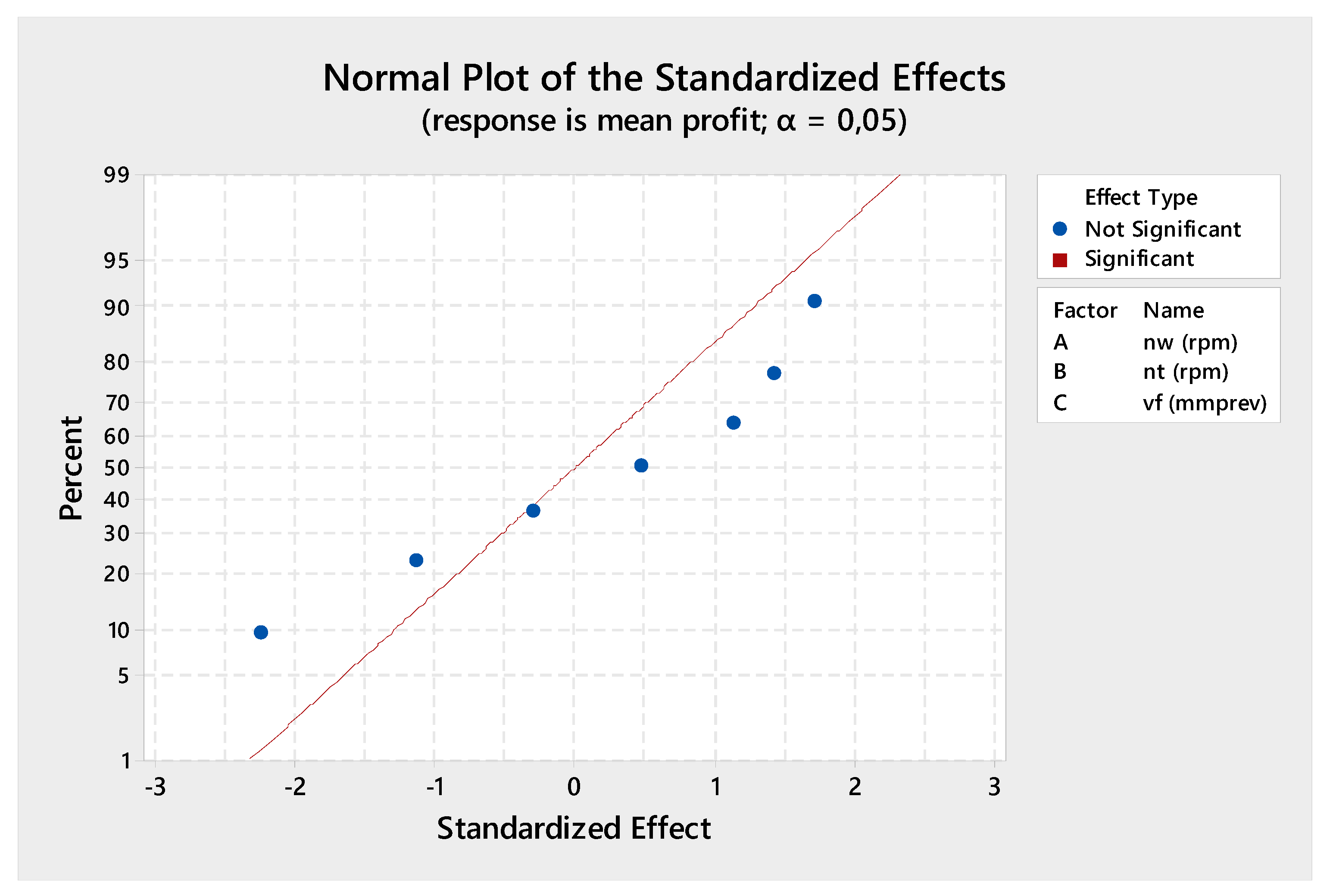
| Term | Effect | Coef. | SE Coef. | t-Value | p-Value | VIF |
|---|---|---|---|---|---|---|
| Constant | 3.064 | 0.118 | 26.02 | 0.024 | ||
| nw (rpm) | −0.155 | −0.078 | 0.118 | −0.66 | 0.629 | 1.00 |
| nt (rpm) | −0.038 | −0.019 | 0.118 | -0.16 | 0.897 | 1.00 |
| vf (mmprev) | −0.094 | −0.047 | 0.118 | −0.40 | 0.758 | 1.00 |
| nw (rpm) × nt (rpm) | 0.154 | 0.077 | 0.118 | 0.65 | 0.631 | 1.00 |
| nw (rpm) × vf (mmprev) | 0.195 | 0.098 | 0.118 | 0.83 | 0.559 | 1.00 |
| nt (rpm) × vf (mmprev) | 0.175 | 0.088 | 0.118 | 0.74 | 0.593 | 1.00 |
| Model Summary | ||||||
| S | R-sq | |||||
| 0.33304 | 79.59% | |||||
| Regression Equation in Uncoded Units | ||||||
| Mean profit = 3038 − 0.1287 nw + 0.007000 nt − 0.09825 vf + 0.1283 nw × nt + 0.1715 nw × vf + 0.1387 nt × vf − 0.1915 nw × nt × vf | ||||||
| Term | Effect | Coef. | SE Coef. | t-Value | p-Value | VIF |
|---|---|---|---|---|---|---|
| Constant | 0.89313 | 0.00312 | 285.80 | 0.000 | ||
| nw (rpm) | −0.01625 | −0.00813 | 0.00312 | −2.60 | 0.032 | 1.00 |
| nt (rpm) | −0.00125 | −0.00062 | 0.00312 | −0.20 | 0.846 | 1.00 |
| vf (mmprev) | −0.01625 | −0.00813 | 0.00312 | −2.60 | 0.032 | 1.00 |
| nw (rpm) × nt (rpm) | 0.00125 | 0.00062 | 0.00312 | 0.20 | 0.846 | 1.00 |
| nw (rpm) × vf (mmprev) | 0.00625 | 0.00312 | 0.00312 | 1.00 | 0.347 | 1.00 |
| nt (rpm) × vf (mmprev) | −0.00875 | −0.00438 | 0.00312 | −1.40 | 0.199 | 1.00 |
| nw (rpm) × nt (rpm) × vf (mmprev) | −0.01125 | −0.00562 | 0.00312 | −1.80 | 0.110 | 1.00 |
| Regression Equation in Uncoded Units | ||||||
| r = 0.89313 − 0.00813 nw (rpm) − 0.00062 nt (rpm) − 0.00813 vf (mmprev)+ 0.00062 nw (rpm) × nt (rpm) + 0.00312 nw (rpm) × vf (mmprev) − 0.00438 nt (rpm) × vf (mmprev) − 0.00562 nw (rpm) × nt (rpm) × vf (mmprev) | ||||||
| Model Summary | ||||||
| S | R-sq | |||||
| 0.44874 | 87.31% | |||||
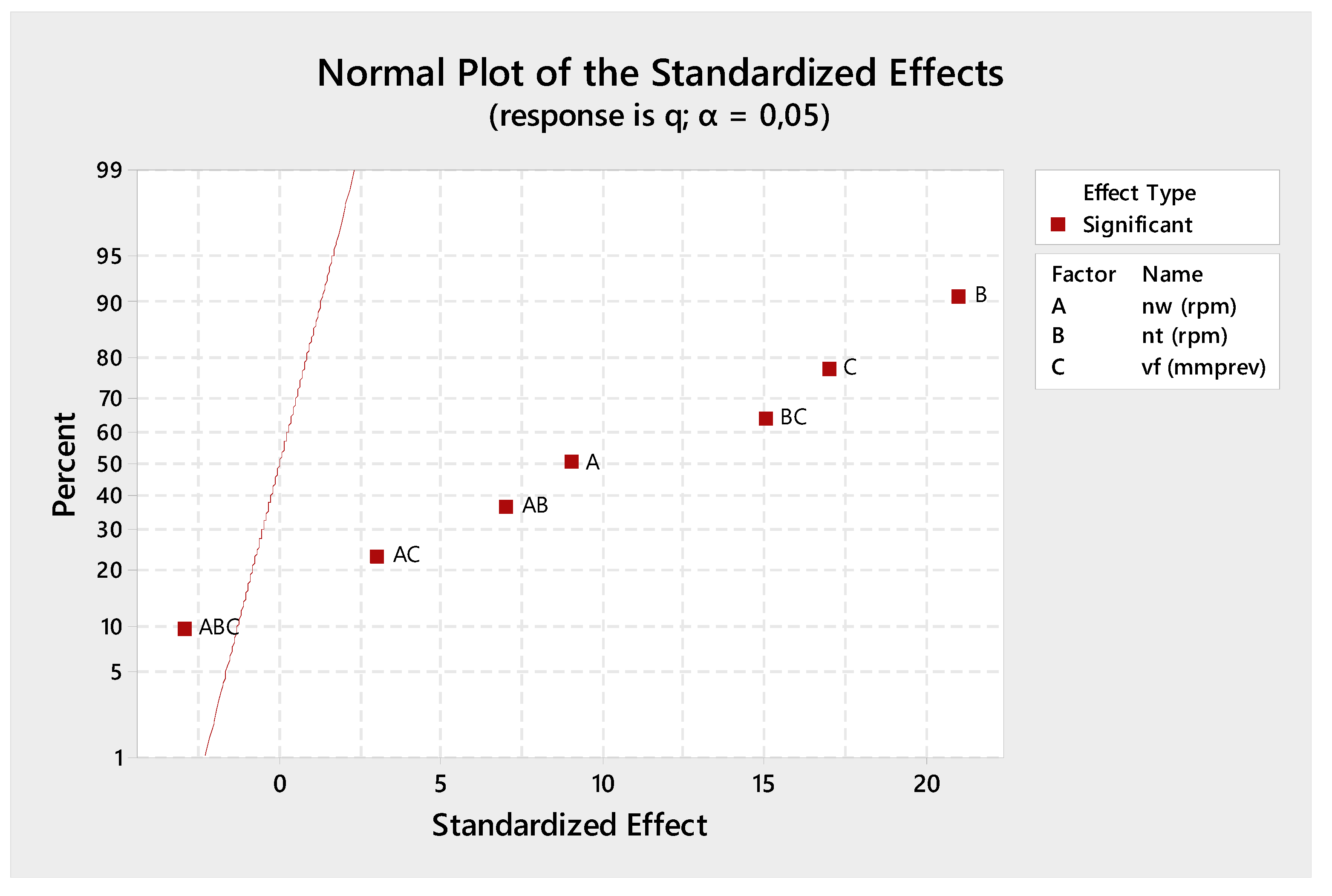
| Term | Effect | Coef. | SE Coef. | t-Value | p-Value | VIF |
|---|---|---|---|---|---|---|
| Constant | 65,700 | 300 | 219.00 | 0.000 | ||
| nw (rpm) | 5400 | 2700 | 300 | 9.00 | 0.000 | 1.00 |
| nt (rpm) | 12,600 | 6300 | 300 | 21.00 | 0.000 | 1.00 |
| vf (mmprev) | 10,200 | 5100 | 300 | 17.00 | 0.000 | 1.00 |
| nw (rpm) × nt (rpm) | 4200 | 2100 | 300 | 7.00 | 0.000 | 1.00 |
| nw (rpm) × vf (mmprev) | 1800 | 900 | 300 | 3.00 | 0.017 | 1.00 |
| nt (rpm) × vf (mmprev) | 9000 | 4500 | 300 | 15.00 | 0.000 | 1.00 |
| nw (rpm) × nt (rpm) × vf (mmprev) | −1800 | −900 | 300 | −3.00 | 0.017 | 1.00 |
| Regression Equation in Uncoded Units. | ||||||
| q = 65,700 + 2700 nw (rpm) + 6300 nt (rpm) + 5100 vf (mmprev) + 2100 nw (rpm) × nt (rpm)+ 900 nw (rpm) × vf (mmprev) + 4500 nt (rpm) × vf (mmprev) − 900 nw (rpm) × nt (rpm) × vf (mmprev) | ||||||
| Model Summary | ||||||
| S | R-sq | |||||
| 0.39170 | 82.58% | |||||
Publisher’s Note: MDPI stays neutral with regard to jurisdictional claims in published maps and institutional affiliations. |
© 2020 by the authors. Licensee MDPI, Basel, Switzerland. This article is an open access article distributed under the terms and conditions of the Creative Commons Attribution (CC BY) license (http://creativecommons.org/licenses/by/4.0/).
Share and Cite
Macak, T.; Hron, J.; Stusek, J. A Causal Model of the Sustainable Use of Resources: A Case Study on a Woodworking Process. Sustainability 2020, 12, 9057. https://doi.org/10.3390/su12219057
Macak T, Hron J, Stusek J. A Causal Model of the Sustainable Use of Resources: A Case Study on a Woodworking Process. Sustainability. 2020; 12(21):9057. https://doi.org/10.3390/su12219057
Chicago/Turabian StyleMacak, Tomas, Jan Hron, and Jaromir Stusek. 2020. "A Causal Model of the Sustainable Use of Resources: A Case Study on a Woodworking Process" Sustainability 12, no. 21: 9057. https://doi.org/10.3390/su12219057
APA StyleMacak, T., Hron, J., & Stusek, J. (2020). A Causal Model of the Sustainable Use of Resources: A Case Study on a Woodworking Process. Sustainability, 12(21), 9057. https://doi.org/10.3390/su12219057