Ageing and Cooling of Hot-Mix-Asphalt during Hauling and Paving—A Laboratory and Site Study


Abstract
1. Introduction
2. Objectives and Experimental Program
2.1. Research Purposes
- (1)
- investigating the ageing that happens during HMA hauling as a function of time and type of truck and
- (2)
- highlighting the issues related to temperature segregation of HMA during paving operations.
2.2. Test Methods
2.2.1. Volumetric Analysis
2.2.2. Indirect Tensile Stiffness Modulus Test
2.2.3. Temperature Monitoring
2.2.4. Indirect Tensile Strength Test
2.2.5. Determination of Cracking Tolerance Index
3. Effect of Conditioning Time in the Oven on Lab-Mixed HMA
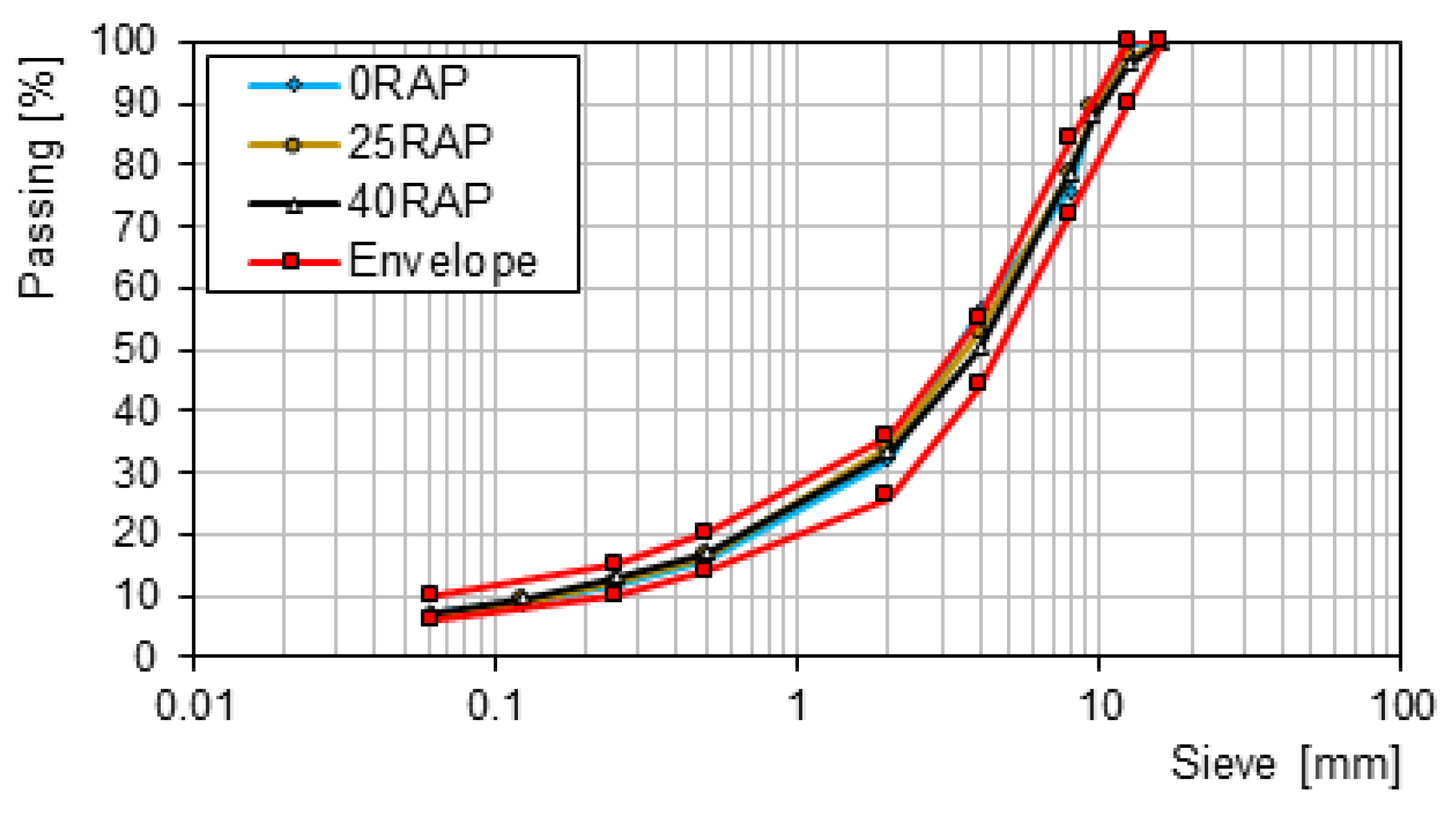
3.1. Materials and Specimen Preparation
3.2. Results and Discussion from the Lab Investigation
4. Effect of Hauling Time and Truck Type on Plant-Mixed HMA
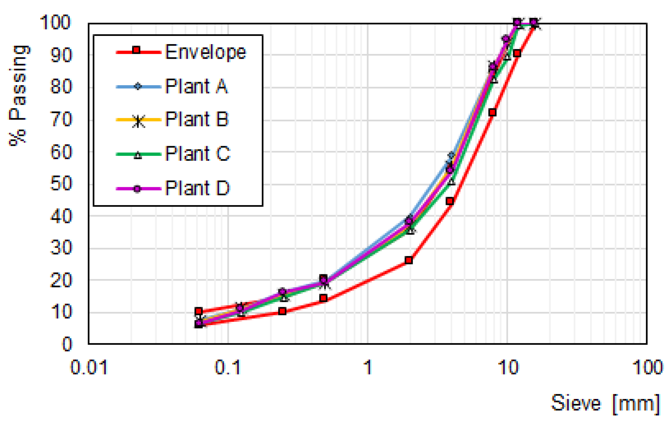
4.1. Mix Properties
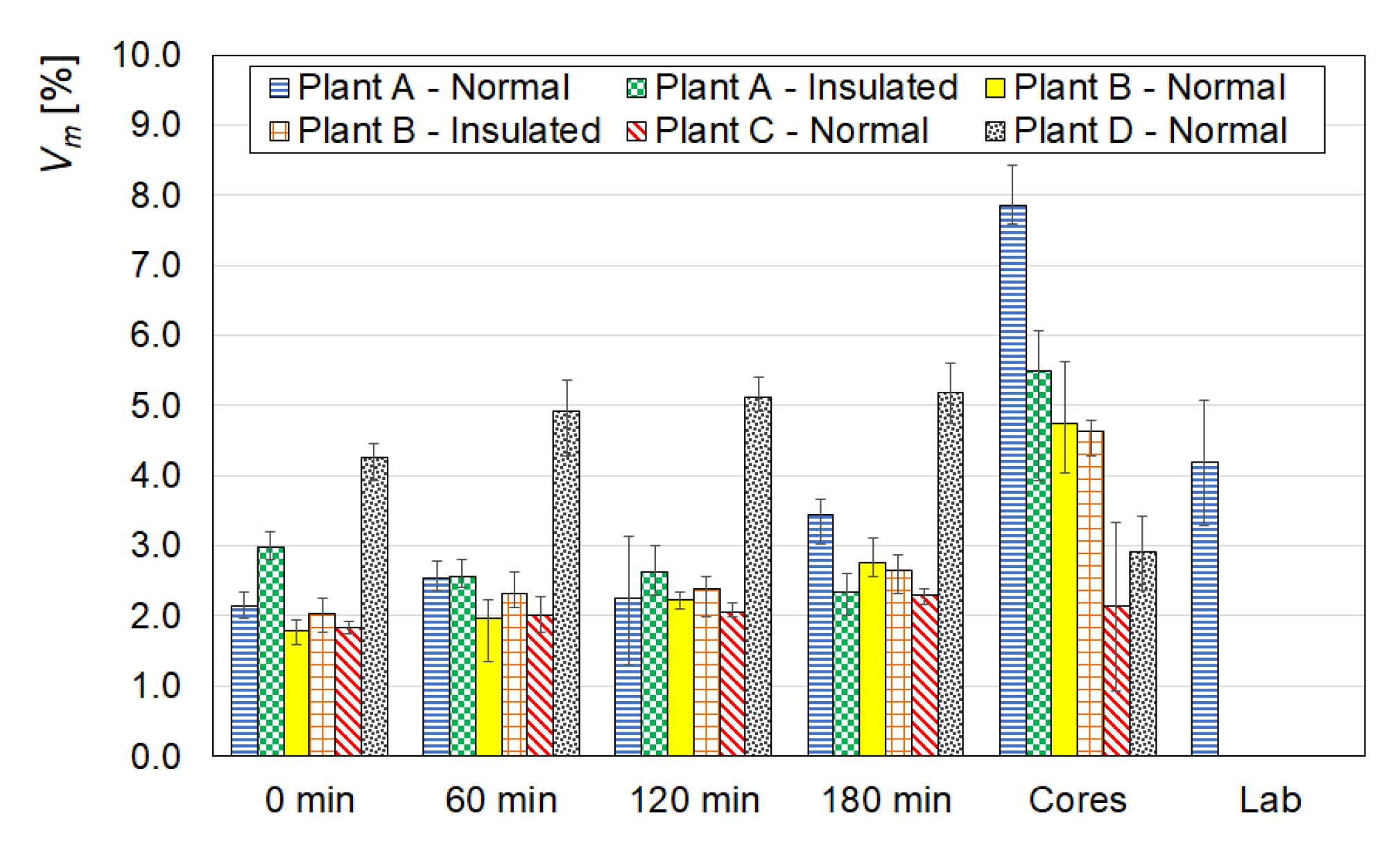
4.2. Result and Discussion from the Site Investigation
4.2.1. Evaluation of Temperatures during Hauling and Paving
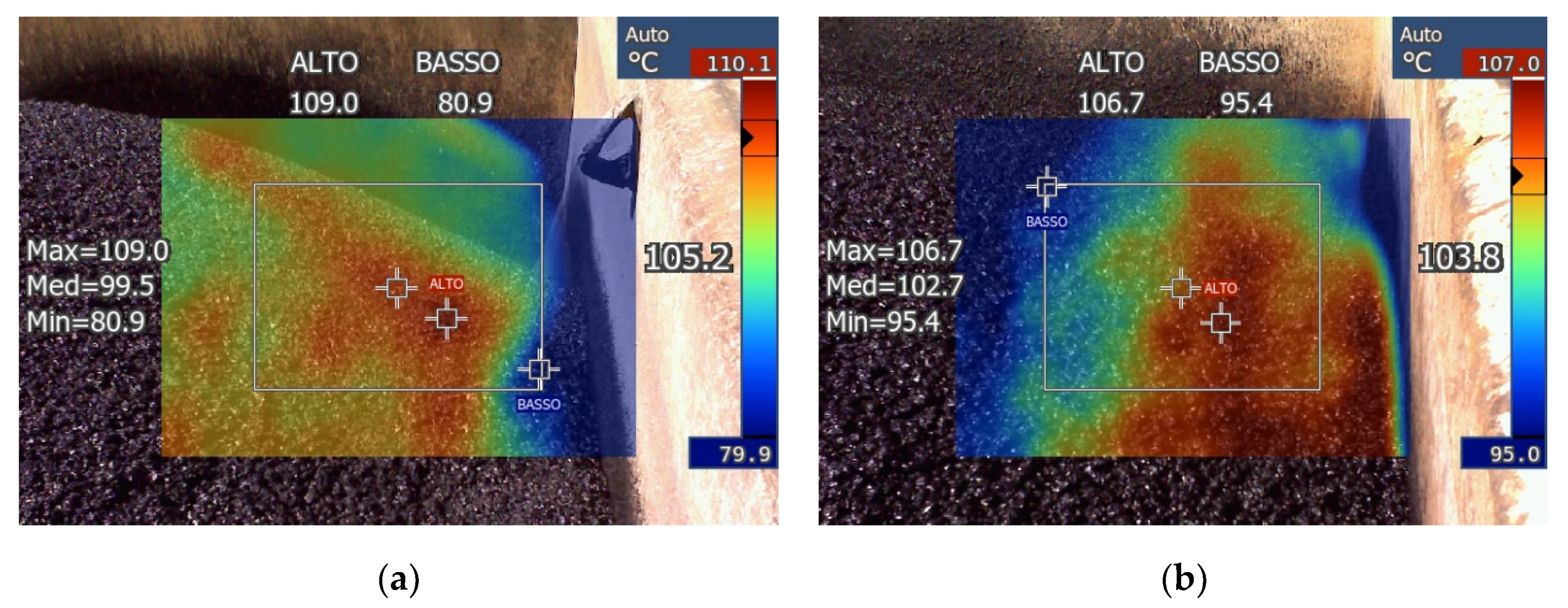
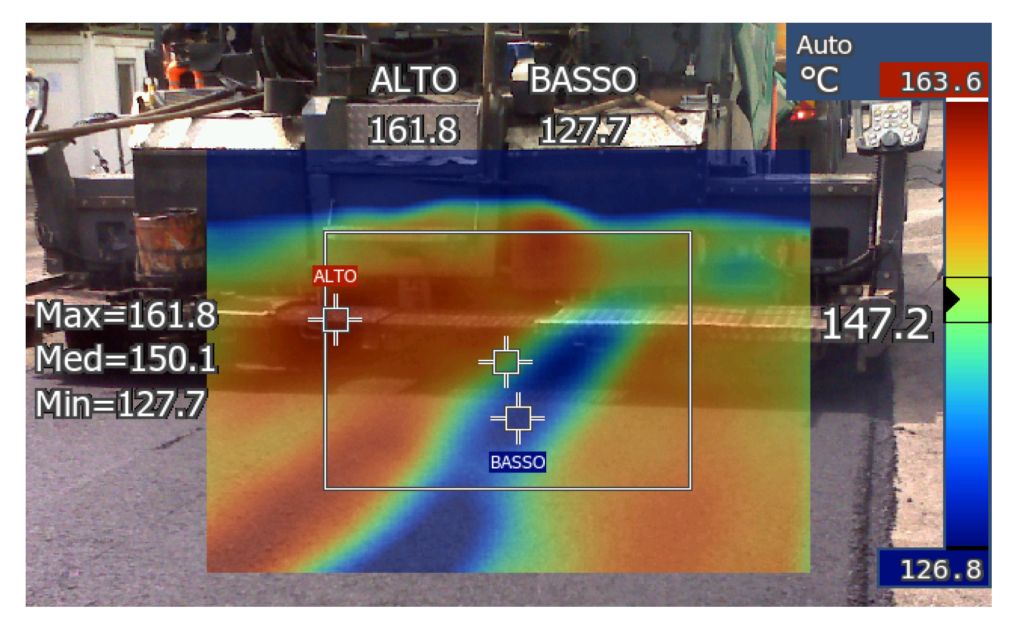
4.2.2. Thermal Image Analysis
4.2.3. Laboratory Tests
5. Conclusions
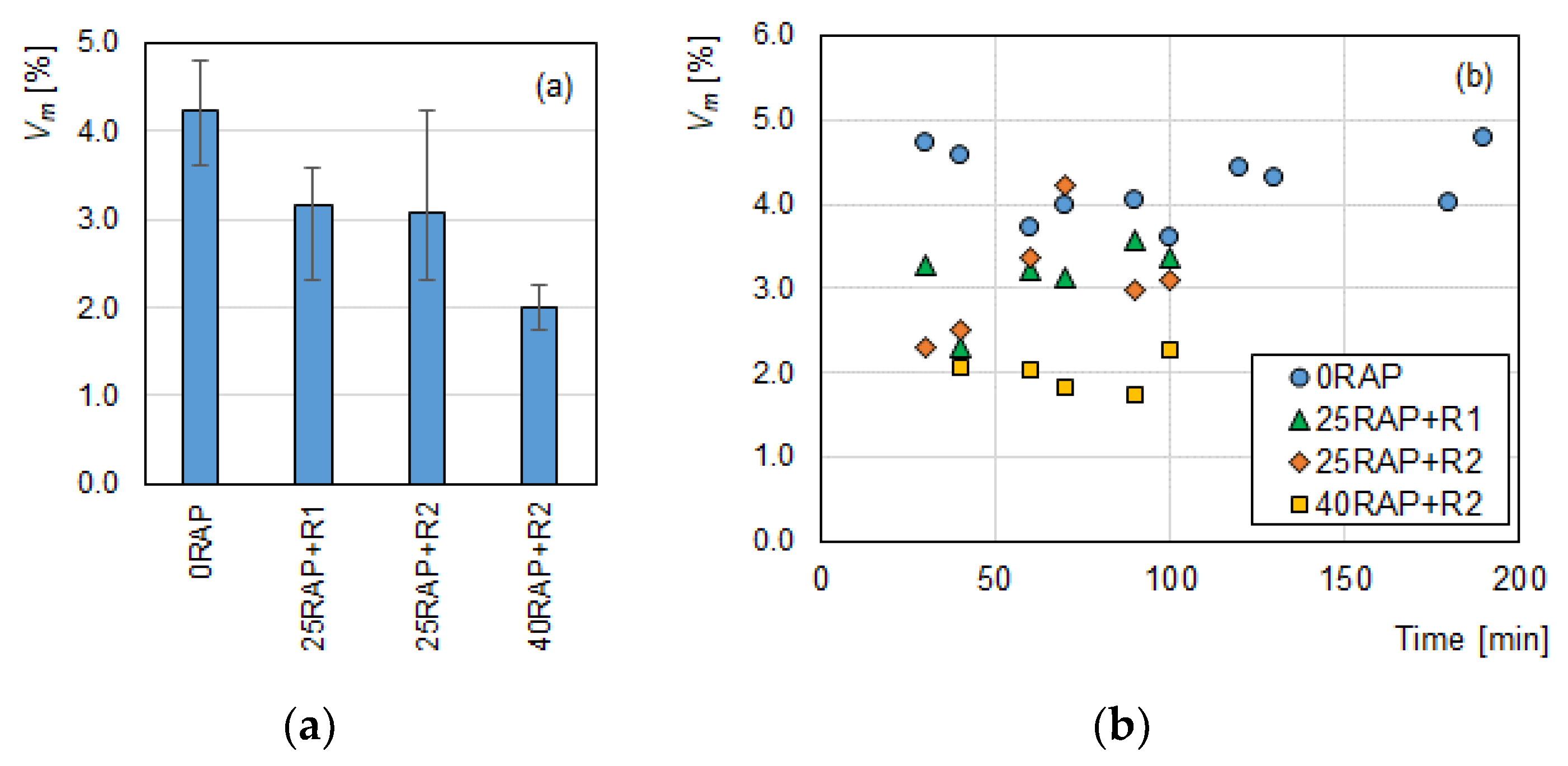
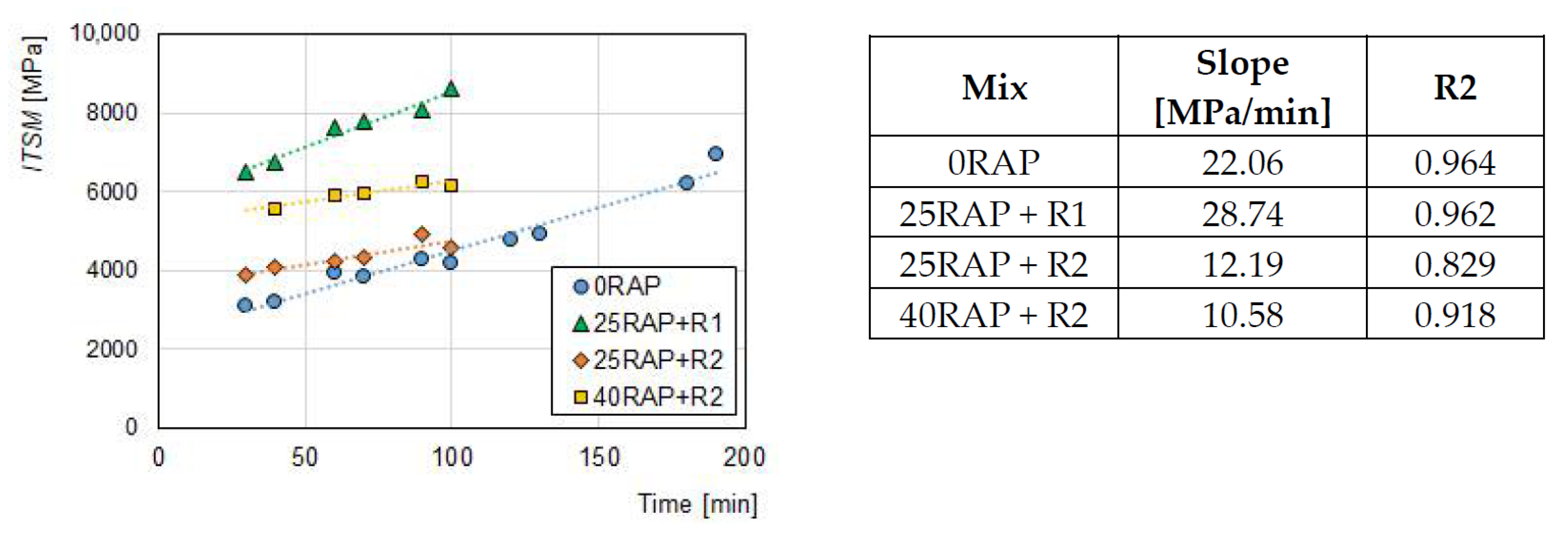
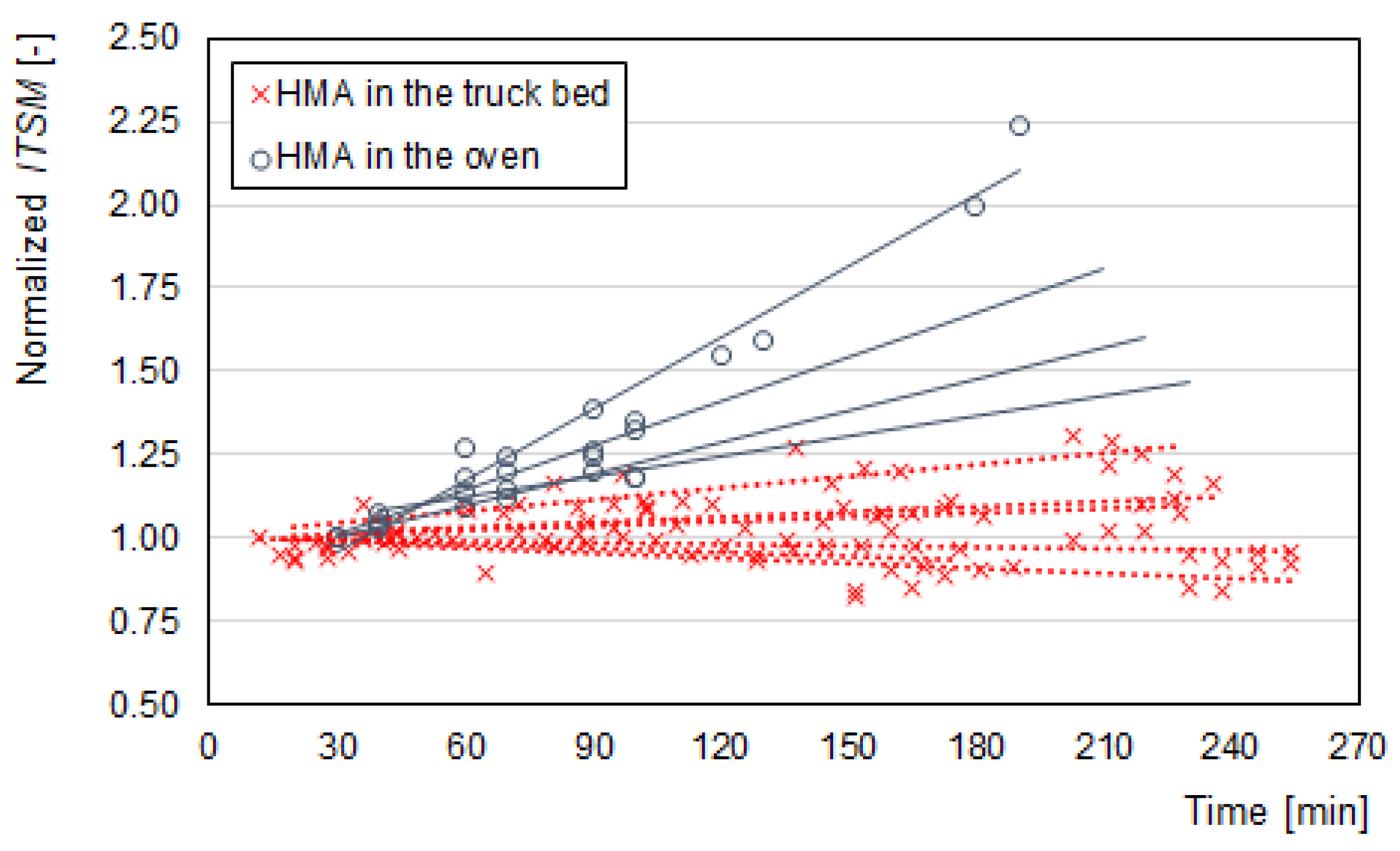
- the compactability of the HMA was not influenced by the time during which the material is conditioned in the oven before compaction. Conversely, all the mixtures tested showed a rising trend of stiffness when the conditioning time was increased. The growing rate was higher for the mix with no RAP (22.1 MPa/min) with respect to those including RAP and a special bitumen engineered for hot recycling applications (12.2 and 10.6 MPa/min respectively for the mix with 25% RAP and 40% RAP);
- the temperature monitoring proved that the mix inside the truck bed did not significantly cool after 3 h of hauling (temperature decrease between 6 °C and 16 °C), while the temperatures on the top corner of the truck and those measured on the sampled loose mix considerably decreased (approximately 60 °C cooling);
- the thermal camera images highlighted a large temperature segregation at the paving site, with discrepancies higher than 30 °C both on the truck bed (normal truck) and on the road surface after paving. However, in the case of the insulated truck the severity of this phenomenon was reduced;
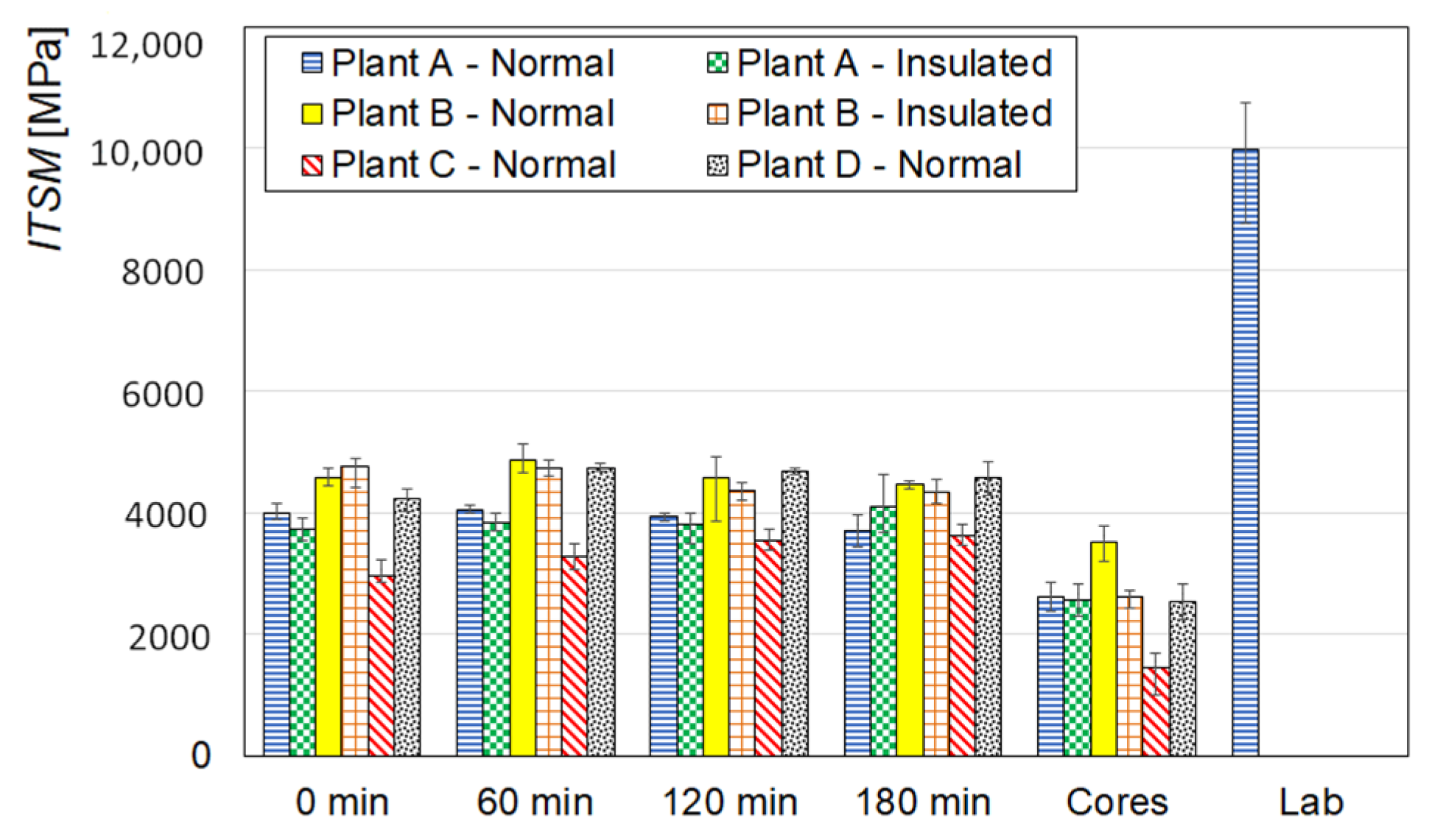
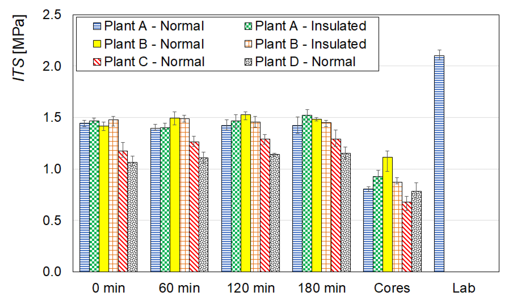
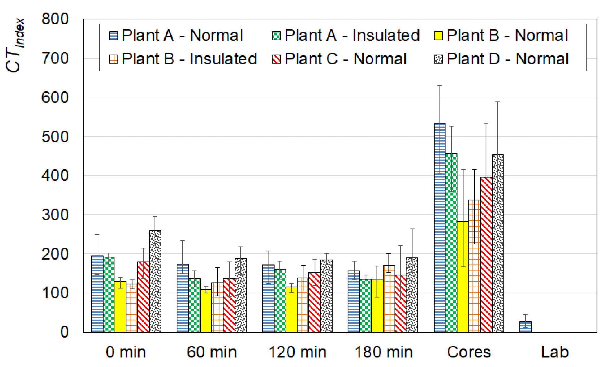
- HMA compactability, stiffness, strength and cracking tolerance did not change when hauling time increased. Inversely from the laboratory oven (where most of the HMA volume was exposed to air), the core of the HMA in the truck bed was basically isolated by the surface material and neither oxidation nor loss of volatility could occur, hindering the ageing of the HMA;
- the cores showed lower ITSM (−39% on average) and ITS (−37% on average) and higher CTindex (about 2.5 times on average) with respect to the specimens compacted on site, probably due to a higher air voids content;
- when the loose HMA was re-heated and compacted in the laboratory, ITSM and ITS (+150% and +50%, respectively) considerably increased, whereas CTIndex decreased (−84%), denoting that a severe ageing happened through this specimen preparation procedure.
Author Contributions
Funding
Conflicts of Interest
References
- Kök, B.V.; Yilmaz, M.; Alatas, T. Evaluation of the mechanical properties of field and laboratory Compacted hot-mix asphalt. J. Mater. Civ. Eng. 2014, 26. [Google Scholar] [CrossRef]
- Morovatdar, A.; Ashtiani, R.S.; Licon, C. Development of a mechanistic framework to predict pavement service life using axle load spectra from Texas overload corridors. In Proceedings of the International Conference on Transportation and Development 2020, Seattle, WA, USA, 26–29 May 2020. [Google Scholar]
- Lu, X.; Isacsson, U. Effect of ageing on bitumen chemistry and rheology. Constr. Build. Mater. 2002, 16, 15–22. [Google Scholar] [CrossRef]
- Miró, R.; Martínez, A.H.; Moreno-Navarro, F.; Rubio-Gámez, C. Effect of ageing and temperature on the fatigue behaviour of bitumens. Mater. Des. 2015, 86, 129–137. [Google Scholar] [CrossRef]
- Hung, A.M.; Fini, E.H. Absorption spectroscopy to determine the extent and mechanisms of aging in bitumen and asphaltenes. Fuel 2019, 242, 408–415. [Google Scholar] [CrossRef]
- Le Guern, M.; Chailleux, E.; Farcas, F.; Dreessen, S.; Mabille, I. Physico-chemical analysis of five hard bitumens: Identification of chemical species and molecular organization before and after artificial aging. Fuel 2010, 89, 3330–3339. [Google Scholar] [CrossRef]
- Mousavi, M.; Pahlavan, F.; Oldham, D.; Hosseinnezhad, S.; Fini, E.H. Multiscale investigation of oxidative aging in biomodified asphalt binder. J. Phys. Chem. C 2016, 120, 17224–17233. [Google Scholar] [CrossRef]
- Mirwald, J.; Werkovits, S.; Camargo, I.; Maschauer, D.; Hofko, B.; Grothe, H. Understanding bitumen ageing by investigation of its polarity fractions. Constr. Build. Mater. 2020, 250, 118809. [Google Scholar] [CrossRef]
- Siddiqui, M.N.; Ali, M.F. Studies on the aging behavior of the Arabian asphalts. Fuel 1999, 78, 1005–1015. [Google Scholar] [CrossRef]
- Lemarchand, C.A.; Schrøder, T.B.; Dyre, J.C.; Hansen, J.S. Cooee bitumen: Chemical aging. J. Chem. Phys. 2013, 139. [Google Scholar] [CrossRef]
- Pahlavan, F.; Samieadel, A.; Deng, S.F.E. Exploiting synergistic effects of intermolecular interactions to synthesize hybrid rejuvenators to revitalize aged asphalt. ACS Sustain. Chem. Eng. 2019, 7, 15514–15525. [Google Scholar] [CrossRef]
- Lesueur, D.; Gerard, J.-F.; Claudy, P.; Letoffe, J.-M.; Planche, J.-P.; Martin, D. Structure related model to describe asphalt linear viscoelasticity. J. Rheol. 1996, 40, 813–836. [Google Scholar] [CrossRef]
- Ongel, A.; Hugener, M. Impact of rejuvenators on aging properties of bitumen. Constr. Build. Mater. 2015, 94, 467–474. [Google Scholar] [CrossRef]
- Mazzoni, G.; Bocci, E.; Canestrari, F. Influence of rejuvenators on bitumen ageing in hot recycled asphalt mixtures. J. Traffic Transp. Eng. Engl. Ed. 2018, 5, 157–168. [Google Scholar] [CrossRef]
- Nakhaei, M.; Ziari, H.; Korayem, A.H.; Hajiloo, M. Aging evaluation of amorphous carbon-modified asphalt binders using rheological and chemical approach. J. Mater. Civ. Eng. 2020, 32. [Google Scholar] [CrossRef]
- Hofko, B.; Falchetto, A.C.; Grenfell, J.; Huber, L.; Lu, X.; Porot, L.; You, Z.; Falchetto, A.C. Effect of short-term ageing temperature on bitumen properties. Road Mater. Pavement Des. 2017, 18, 108–117. [Google Scholar] [CrossRef]
- Dessouky, S.; Reyes, C.; Ilias, M.; Contreras, D.; Papagiannakis, A.T. Effect of pre-heating duration and temperature conditioning on the rheological properties of bitumen. Constr. Build. Mater. 2011, 25, 2785–2792. [Google Scholar] [CrossRef]
- Lolly, R.; Zeiada, W.; Souliman, M.; Kaloush, K. Effects of short-term aging on asphalt binders and hot mix asphalt at elevated temperatures and extended Aging Time. MATEC Web Conf. 2017, 07010. [Google Scholar] [CrossRef]
- Lemke, Z.; Sadek, H.; Swiertz, D.; Reichelt, S.; Bahia, H.U. Effects of reheating procedure and oven type on performance testing results of asphalt mixtures. Transp. Res. Rec. 2018, 2672, 124–133. [Google Scholar] [CrossRef]
- Kidd, A.; Stephenson, G.; White, G. Implications of reheating of asphalt mixes on performance testing. In Proceedings of the 18th AAPA International Flexible Pavements Conference 2019, Sydney, New South Wales, Australia, 18–21 August 2019. [Google Scholar]
- Daniel, J. How mixture, fabrication, and plant production parameters affect mixture properties. Transp. Res. Circ. 2018, E-C234, 1–20. [Google Scholar]
- Roberts, F.L.; Kandhal, P.S.; Brown, E.R.; Lee, D.Y.; Kennedy, T.W. Hot Mix Asphalt Materials, Mixture Design, and Construction, 3rd ed.; National Asphalt Paving Association Education Foundation: Lanham, MD, USA, 2016. [Google Scholar]
- Muhammad, M.; Syuhada, A.; Huzni, S.; Fuadi, Z. Study on Heat loss through dump truck wall insulated by sengon wood. J. Adv. Res. Fluid Mech. Therm. Sci. 2019, 58, 126–134. [Google Scholar]
- Cho, Y.K.; Bode, T.; Song, J.; Jeong, J.-H. Thermography-driven distress prediction from hot mix asphalt road paving construction. ASCE J. Constr. Eng. Manag. 2012, 138, 206–214. [Google Scholar] [CrossRef]
- Mahoney, J.P.; Muench, S.T.; Pierce, L.M.; Read, S.A.; Jakob, H.; Moore, R. Construction-related temperature differentials in asphalt concrete pavement: Identification and assessment. Transp. Res. Rec. 2000, 1712, 93–100. [Google Scholar] [CrossRef]
- Amirkhanian, S.N.; Putman, B.J. Laboratory and Field Investigation of Temperature Differential in HMA Mixtures Using an Infrared Camera; Clemson University Department of Civil Engineering: Clemson, SC, USA, 2006. [Google Scholar]
- Brock, J.D.; Jakob, H. Temperature Segregation/Temperature Differential Damage; Technical Paper T-134; Astec Industries: Chattanooga, TN, USA, 2009. [Google Scholar]
- Kim, M.; Phaltane, P.; Mohammad, L.N.; Elseifi, M. Temperature segregation and its impact on the quality and performance of asphalt pavements. Front. Struct. Civ. Eng. 2017, 12, 536–547. [Google Scholar] [CrossRef]
- Delgadillo, R.; Bahia, H.U. Effects of temperature and pressure on hot mixed asphalt compaction: Field and laboratory study. J. Mater. Civ. Eng. 2008, 20, 440–448. [Google Scholar] [CrossRef]
- Hayat, A.; Hussain, A.; Afridi, H.F. Determination of in-field temperature variations in fresh HMA and corresponding compaction temperatures. Constr. Build. Mater. 2019, 216, 84–92. [Google Scholar] [CrossRef]
- Khan, R.; Grenfell, J.; Collop, A.; Airey, G.; Gregory, H. Moisture damage in asphalt mixtures using the modified SATS test and image analysis. Constr. Build. Mater. 2013, 43, 165–173. [Google Scholar] [CrossRef]
- Plati, C.; Georgiou, P.; Loizos, A. Use of infrared thermography for assessing HMA paving and compaction. Transp. Res. Part C Emerg. Technol. 2014, 46, 192–208. [Google Scholar] [CrossRef]
- Bocci, E.; Mazzoni, G.; Canestrari, F. Ageing of rejuvenated bitumen in hot recycled bituminous mixtures: Influence of bitumen origin and additive type. Road Mater. Pavement Des. 2019, 20, 127–148. [Google Scholar] [CrossRef]
- Test Methods for Hot Mix Asphalt. Part 31: Specimen Preparation by Gyratory Compactor; EN 12697-31; European Committee for Standardization (CEN): Brussels, Belgium, 2019.
- Test Methods for Hot Mix Asphalt. Part 8: Determination of Void Characteristics of Bituminous Specimens; EN 12697-8; European Committee for Standardization (CEN): Brussels, Belgium, 2019.
- Test Methods for Hot Mix Asphalt. Part 5: Determination of the Maximum Density; EN 12697-5; European Committee for Standardization (CEN): Brussels, Belgium, 2019.
- Test Methods for hot Mix Asphalt. Part 6: Determination of the Bulk Density of Bituminous Specimens; EN 12697-6; European Committee for Standardization (CEN): Brussels, Belgium, 2020.
- Cerni, G.; Bocci, E.; Cardone, F.; Corradini, A. Correlation between asphalt mixture stiffness determined through static and dynamic indirect tensile tests. Arab. J. Sci. Eng. 2017, 42. [Google Scholar] [CrossRef]
- Test Methods for Hot Mix Asphalt. Part 26: Stiffness; EN 12697-26; European Committee for Standardization (CEN): Brussels, Belgium, 2018.
- Graziani, A.; Bocci, E.; Canestrari, F. Bulk and shear characterization of bituminous mixtures in the linear viscoelastic domain. Mech. Time Depend. Mater. 2014, 18, 527–554. [Google Scholar] [CrossRef]
- Test Methods for Hot Mix Asphalt. Part 23: Determination of the Indirect Tensile Strength of Bituminous Specimens; EN 12697-23; European Committee for Standardization (CEN): Brussels, Belgium, 2017.
- Standard Test Method for Determination of Cracking Tolerance Index of Asphalt Mixture Using the Indirect Tensile Cracking Test at Intermediate Temperature; ASTM D8225-19; ASTM International: West Conshohocken, PA, USA, 2019. [CrossRef]
- Zhou, F.; Im, S.; Sun, L.; Scullion, T. Development of an IDEAL cracking test for asphalt mix design and QC/QA. Road Mater. Pavement Des. 2017, 18, 405–427. [Google Scholar] [CrossRef]
- Direttive Tecniche per Pavimentazioni Bituminose; Amministrazione Provincia Bolzano: Bolzano, Italy, 2016. (In Italian)
- Framework Specification for Polymer Modified Bitumens; EN 14023; European Committee for Standardization (CEN): Brussels, Belgium, 2010.
- Test Methods for Hot Mix Asphalt. Part 35: Laboratory Mixing; EN 12697-35; European Committee for Standardization (CEN): Brussels, Belgium, 2016.


| Mix | RAP Content [%] | Rejuvenating Technique | Conditioning Time [min] | Conditioning Temperature [°C] |
|---|---|---|---|---|
| 0RAP | 0 | - | 30, 60, 90, 120, 180 | 180 |
| 25RAP-R1 | 25 | R1 | 30, 60, 90 | 180 |
| 25RAP-R2 | 25 | R2 | 30, 60, 90 | 180 |
| 40RAP-R2 | 40 | R2 | 30, 60, 90 | 180 |
| Plant A | Plant B | Plant C | Plant D | ||
|---|---|---|---|---|---|
| Truck | Normal | X | X | X | X |
| Insulated | X | X | |||
| Specimens compacted on site | After 0 h hauling | X | X | X | X |
| After 1 h hauling | X | X | X | X | |
| After 2 h hauling | X | X | X | X | |
| After 3 h hauling | X | X | X | X | |
| Cores | X | X | X | ||
| Specimens compacted in the lab after reheating | X | ||||
| Plant | A | B | C | D |
|---|---|---|---|---|
| Binder content [% by mix] | 6.10 | 6.45 | 6.60 | 5.55 |
| Plant | Truck | Production | 1st Sampling | 2nd Sampling | 3rd Sampling | 4th Sampling | ||
|---|---|---|---|---|---|---|---|---|
| A | Normal | Hours | 9:00 | 9:12 | 10:08 | 11:04 | 11:27 | |
| T [°C] | C | - | 146 | 121 | 98 | 87 | ||
| B | - | 184 | 175 | 171 | 168 | |||
| L | - | 165 | 160 | 152 | 146 | |||
| Insulated | Hours | 9:00 | 9:40 | 10:37 | 11:33 | 12:27 | ||
| T [°C] | C | - | 143 | 124 | 105 | 101 | ||
| B | - | 178 | 182 | 170 | 165 | |||
| L | - | 165 | 160 | 163 | 154 | |||
| B | Normal | Hours | 8:45 | 8:52 | 9:59 | 10:56 | 12:30 | |
| T [°C] | C | - | 152 | 112 | 100 | 94 | ||
| B | - | 181 | 186 | 184 | 175 | |||
| L | - | 150 | 138 | 131 | 110 | |||
| Insulated | Hours | 8:45 | 9:21 | 10:25 | 11:25 | 12:30 | ||
| T [°C] | C | - | 133 | 106 | 92 | 96 | ||
| B | - | 182 | 185 | 180 | 172 | |||
| L | - | 165 | 151 | 131 | 111 | |||
| C | Normal | Hours | 9:00 | 9:15 | 10:08 | 11:13 | 12:18 | |
| T [°C] | C | - | 135 | 101 | 90 | 87 | ||
| B | - | 185 | 183 | 178 | 174 | |||
| L | - | 147 | 160 | 137 | 117 | |||
| D | Normal | Hours | 8:00 | 8:15 | 9:22 | 10:24 | 11:18 | |
| T [°C] | C | - | 151 | 109 | 97 | 85 | ||
| B | - | 188 | 188 | 186 | 182 | |||
| L | - | 169 | 130 | 129 | 109 | |||
| A | B | C | D | |||
|---|---|---|---|---|---|---|
| N | I | N | I | N | N | |
| Time elapsed between production and lay-down [min] | 210 | 242 | 203 | 230 | 242 | 196 |
| Temperature of the loose mix in the paver [°C] | - | - | 180 | 172 | 121 | 170 |
| Surface HMA temperature after lay-down (probe) [°C] | - | - | 161 | 140 | 106 | 152 |
| Surface HMA temperature after lay-down (infrared) [°C] | - | - | 146 | 181 | 142 | 171 |
| Temperature of outside of the truck bed [°C] | - | - | 62 | 155 | 55 | 62 |
| Temperature of bottom of the truck bed [°C] | - | - | 55 | - | 75 | 81 |
| Variable | |||
|---|---|---|---|
| Property | Truck Type | Sampling Time | HMA Manufacturing Plant |
| Vm | 0.438 | 0.235 | 7.0 × 10⁻²⁵ |
| ITSM | 0.552 | 0.615 | 9.7 × 10⁻²² |
| ITS | 0.266 | 0.655 | 6.9 × 10⁻²⁷ |
| CTIndex | 0.967 | 0.032 | 5.0 × 10⁻⁷ |
Publisher’s Note: MDPI stays neutral with regard to jurisdictional claims in published maps and institutional affiliations. |
© 2020 by the authors. Licensee MDPI, Basel, Switzerland. This article is an open access article distributed under the terms and conditions of the Creative Commons Attribution (CC BY) license (http://creativecommons.org/licenses/by/4.0/).
Share and Cite
Bocci, E.; Prosperi, E.; Mair, V.; Bocci, M. Ageing and Cooling of Hot-Mix-Asphalt during Hauling and Paving—A Laboratory and Site Study. Sustainability 2020, 12, 8612. https://doi.org/10.3390/su12208612
Bocci E, Prosperi E, Mair V, Bocci M. Ageing and Cooling of Hot-Mix-Asphalt during Hauling and Paving—A Laboratory and Site Study. Sustainability. 2020; 12(20):8612. https://doi.org/10.3390/su12208612
Chicago/Turabian StyleBocci, Edoardo, Emiliano Prosperi, Volkmar Mair, and Maurizio Bocci. 2020. "Ageing and Cooling of Hot-Mix-Asphalt during Hauling and Paving—A Laboratory and Site Study" Sustainability 12, no. 20: 8612. https://doi.org/10.3390/su12208612
APA StyleBocci, E., Prosperi, E., Mair, V., & Bocci, M. (2020). Ageing and Cooling of Hot-Mix-Asphalt during Hauling and Paving—A Laboratory and Site Study. Sustainability, 12(20), 8612. https://doi.org/10.3390/su12208612