Article

Measuring Intra-Urban Inequality with Structural Equation Modeling: A Theory-Grounded Indicator

by
Matheus Pereira Libório
1,*,
Oseias da Silva Martinuci
2,
Sandro Laudares
3,
Renata de Mello Lyrio
4,
Alexei Manso Correa Machado
5,6,
Patrícia Bernardes
1 and
Petr Ekel
7,8
1
Department of Administration, Pontifical Catholic University of Minas Gerais, Belo Horizonte, MG 30535-012, Brazil
2
Department of Geography, Maringá State University, Maringá, PR 87000-000, Brazil
3
Department of Geography, Pontifical Catholic University of Minas Gerais, Belo Horizonte, MG 30535-012, Brazil
4
School of Information Science, Federal University of Minas Gerais, Belo Horizonte, MG 31270-901, Brazil
5
Department of Computer Science, Pontifical Catholic University of Minas Gerais, Belo Horizonte, MG 30535-901, Brazil
6
Department of Anatomy and Imaging, Federal University of Minas Gerais, Belo Horizonte, MG 30130-100, Brazil
7
Department of Electrical Engineering, Pontifical Catholic University of Minas Gerais, Belo Horizonte, MG 30535-012, Brazil
8
Department of Electrical Engineering, Federal University of Minas Gerais, Belo Horizonte, MG 31270-901, Brazil
*
Author to whom correspondence should be addressed.
Sustainability 2020, 12(20), 8610; https://doi.org/10.3390/su12208610
Submission received: 8 September 2020 / Revised: 12 October 2020 / Accepted: 13 October 2020 / Published: 17 October 2020
(This article belongs to the Section Sustainability in Geographic Science)

Abstract

:
Composite indicators are almost always determined by methods that aggregate a reasonable number of manifest variables that can be weighted—or not—as new synthesis variables. A problem arises when these aggregations and weightings do not capture the possible effects that the various underlying dimensions of the phenomenon have on each other, and consequently distort the assessment of intra-urban inequality. In this paper, we explore the direct and indirect effects that the different underlying dimensions of intra-urban inequality have on indicators that represent this phenomenon. Structural equation modeling was used to build a composite indicator that captures the direct and indirect effects of the underlying dimensions of intra-urban inequality. From this modeling that combines confirmatory factor analysis with a system of simultaneous equations, the intra-urban inequality of the urban conurbation of Maringá–Sarandi–Paiçandu, Brazil was measured. The model comprises first- and second-order structures. The first-order structure is composed of non-observed variables that represent three underlying dimensions of intra-urban inequality. The second-order structure is the intra-urban inequality composite indicator that synthesizes the non-observed variables of the first-order structure. The model aims at demonstrating how to perform a theorized measurement of urban inequality so that it makes it possible to identify which dimensions most influence the others, as well as which dimensions are more relevant to this purpose.

1. Introduction

Researchers have focused on the development and use of composite indicators to represent complex phenomena [1]. These indicators’ construction is almost always done by methods that aggregate a reasonable number of manifested variables, which can be weighted or not, in a new synthesis variable [2]. The problem is that this aggregation and weighting do not allow one to capture the effects that the multiple underlying dimensions of the phenomenon have on each other. Thus, it is disregarded, for example, that the socioeconomic condition of families influences their housing conditions [3]. This limitation means that intra-urban inequality composite indicators constructed from methods based on aggregation and weighting (e.g., see [4,5]) do not capture the effects among the underlying dimensions of the inequality. Such methods do not allow for consideration of the influence that indicators have on each other, such as socioeconomic [6], neighborhood [7], and household [8] inequalities.
In this context, this research aims to explore the direct and indirect effects that the different underlying dimensions of intra-urban inequality have on the indicator that represents this phenomenon. In order to build a composite indicator that captures the effects of the underlying dimensions of intra-urban inequality, a model that combines confirmatory factor analysis with a model of simultaneous equations [9], known as structural equation modeling [10,11,12], was developed. The model was developed taking as an example the intra-urban inequality of the Maringá–Sarandi–Paiçandu conurbation in Brazil. This model comprises first- and second-order structures. The first-order structure is composed of non-observed variables that represent three underlying dimensions of the intra-urban inequality. The second-order structure is the variable that synthesizes the variables of the first-order structure. From this synthesis variable, the Structured Intra-urban Inequality Indicator (S-III) is expected to contribute to a theorized measurement of intra-urban inequality that considers the interrelationships among the underlying dimensions of this phenomenon.
In addition to this introduction, this article presents urban inequality with its research fronts and some examples of indicators in Section 2. The main foundations of the composite indicators are presented in Section 3. Section 4 presents structural equation modeling, as well as its different variables, models, and relationships. Section 5 presents the research materials and methods, showing the variables and dimensions of the indicator, the characteristics of the model, and the description of the tests necessary to validate the results. Section 6 presents the results, discussions, and contributions to the research, followed by the conclusions, limitations, and suggestions for future work.

2. Urban Inequality

Urban inequality has been studied from unique perspectives, such as, for example, economic [13,14], geographic [15,16,17], and, mainly, sociological perspectives (Bourdieu, 2016; [18,19,20,21]. These perspectives guide researchers and create areas of specialties and different research fronts on urban inequality. However, what are these research fronts and how we identify them?
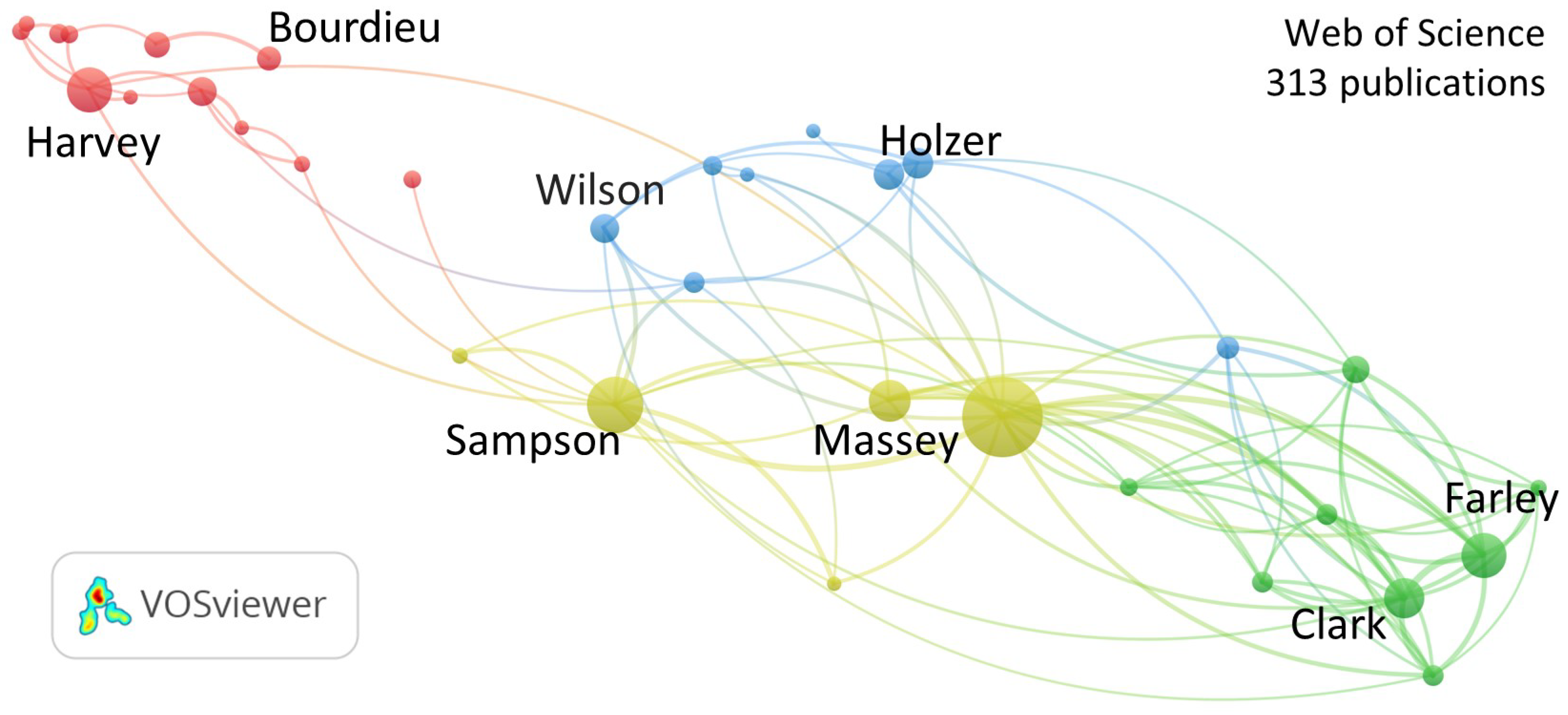
One of the most accurate techniques [22] to identify research fronts [23] is the frequency analysis of co-citation by influential researchers. VOSviewer is a software used to analyze how the most influential authors are cited and organized within the specialized literature [24]. Figure 1 shows the co-citation analysis of 313 publications indexed in the Scopus database that explicitly mention urban inequality.
The analysis of co-citations shows four research fronts on urban inequality. From left to right, the first research front, in red dots, represents works that most frequently cite Harvey [15,16] and Bourdieu (2016). The citation of these authors’ works from this research front indirectly focuses on the study of the dynamics of power in society, as well as the geographic study of urban poverty and its consequences. The second research front, in blue dots, represents researchers that most frequently cite the works of Holzer [13,14] and Wilson [21]. Studies that often mention these authors are indirectly concerned with understanding how geographic characteristics affect the work/employment of low-income people and how the low employment opportunity in the neighborhoods exacerbates poverty. Research associated with the third research front, in yellow dots, cites the works of Massey [18] and Massey and Denton [25], which address the problem of immigration and the effects of urban segregation of blacks, or cite the works of Sampson and Laub [20] and Sampson et al. [19], which are concerned with collective engagement, understanding of crime, the effects of neighborhoods, and the social organization of cities. The fourth and last research front on urban inequality, represented in green dots, is formed by works that most frequently cite the works of Farley and Frey [26] and Clark and Dieleman [17]. Such research focuses on the study of population trends and on the analysis of patterns such as racial and ethnic differences and changes, as well as their effects on the urban housing market.
Differentiated research fronts indicate the recognition that urban inequality is made of different dimensions. In this context, researchers have used composite indicators not only to represent urban inequality [4,5], but also to represent its different dimensions. For example, it is possible to indicate socioeconomic [6,27,28], neighborhood [7,29], and household inequalities [8,30], among others [31,32]. The present research focuses both on the general representation of urban inequality and on its dimensions. It also deals with the relationships and the influences of these dimensions on urban inequalities, which are represented through composite indicators.

3. Composite Indicators

The literature shows that there is no single, consolidated definition of what composite indicators (CIs) are. However, it is possible to state that CIs are a mathematical aggregation of variables, normalized or standardized, weighted or not, in a single indicator capable of representing different dimensions of a complex concept or phenomenon [33,34,35]. There is strong criticism about the aggregation and weighting process for the construction of a CI [36,37], as well as about its ability to measure a complex concept or phenomenon [38]. Even so, CIs have attracted the attention of researchers in an increasing number of publications on varied areas of knowledge [38], including the analysis of intra-urban inequality [1].
A wide variety of methods can be used in the construction of CIs [2]. Regardless of the method, the construction begins with the definition of the structure of individual indicators, which should be sufficient to describe the phenomenon [34]. This decision can be based on expert opinion—for instance, applying an analytic hierarchy process [39]—or on the statistical structure of the data set—e.g., using multivariate analyses [40]. In particular, multivariate analyses are useful for assessing the general structure of individual indicators in order to verify the adequacy of these indicators and to justify methodological choices for weighting and aggregating the variables [34].
Among the many options of multivariate analysis methods used in the construction of CIs, factorial methods are common choices. Cronbach’s coefficient alpha (CA) measures the internal consistency of the pairwise correlations between individual indicators [35,41]. The use of CA allows one to evaluate how well the individual indicators describe multidimensional constructs [34]. The application of principal component analysis (PCA) results in major components that account for a maximum amount of variance in observed variables [42]. PCA is commonly used for dimensionality reduction [43]. Factor analysis (FA) allows for the estimation of latent variables that influence the responses of the observed variables [42]. FA is commonly used to describe the variability between the correlated observed variables in terms of a potentially smaller number of unobserved variables [43]. Correspondence analysis is a non-parametric descriptive/exploratory technique of dimensionality reduction similar to PCA and FA, but applied to categorical data instead of continuous data [35]. Multiple correspondence analysis (MCA) is the extension of simple correspondence analysis applied to data sets with more than two categorical variables [44,45].
These factorial methods measure the degree of similarity between the individual variables, indicating whether the structure of the CI is sufficiently reliable to describe the phenomenon [35]. However, when limiting themselves to aggregating the variables in a CI, these methods disregard the effects that the variables and dimensions of the phenomenon have on each other. For example, they disregard that the income variable influences the infant mortality rate [46] or that the dimension of the housing conditions of families is influenced by the socioeconomic dimension [3].
How can this limitation be overcome? In order for the CI to capture the influence of its multiple dimensions, Cataldo et al. [1] suggest the structuring of latent variable blocks or dimensions that aggregate observed variables of their own and that are related according to the theoretical framework. This model is operationalized through structural equation modeling (SEM) and allows us to answer what the strength and significance of the effects between the dimensions of urban inequality are in the indicator.

4. Structural Equation Modeling (SEM)

The theory of structural equation modeling began with the seminal work of Jöreskog [47] from the design of a model that combines confirmatory factor analysis and a system of simultaneous equations [9]. In summary, this model is formed by two types of variables: the latent variables, which are not observed and represent theoretical concepts or constructs [48,49], and the observed variables, which are the measurable variables that are associated with a concept or construct [50].
SEM allows for the operation of two models: covariance-based structural equation modeling (CB-SEM) and partial least square structural equation modeling (PLS-SEM) [11]. While CB-SEM aims to test, confirm, or compare alternative theories, PLS-SEM aims to explore a theoretical framework [48]. In both cases, the construction of the model is carried out dynamically through the inclusion/exclusion of variables or construction relationships based on three elements. First, the relevance of the variables in the construct is assessed using their factor loads. Second, the strength of the associations between variables and constructs and between constructs is measured using their correlation coefficients. Third, the statistical significance of the relationships is evaluated using a t-test between variables and constructs or between constructs [50].
The model should also consider how the latent and observed variables are related. The relationship between the latent variables and the observed variables will be formative in four situations: first, when the direction of causality is towards the constructs to be built; second, when the observed variables define some characteristics of the construct; third, when changes in the observed variables cause changes in the construct; fourth, when changes in the construct do not cause changes in the observed variables [51]. In addition to these options, when changes in the latent variable influence the measurements of the observed variables, the relationship between the construct and the observed variables will be reflexive [52].
In summary, SEM allows us to assess the strength and significance of the effects between the variables and the dimensions of the construct of interest, and to build an indicator to capture these effects. For example, Park et al. [53] show that the urbanization indicator of the Inner Mongolia region is strongly and significantly influenced by the dimension of economic development, while the Mongolia region is strongly and significantly influenced by the dimensions of social goods and economic development. The literature also brings other examples of works that use PLS-SEM to explore how the dimensions of a phenomenon are related and influence indicators of quality of work [54], fair and sustainable well-being [55], disorder perceived in the neighborhood [56], and social cohesion [31].

5. Materials and Methods

This article presents a case study to explore the direct and indirect effects that the different dimensions of intra-urban inequality have on the S-III that represents such a phenomenon. The studied area is the urban conurbation of Maringá–Sarandi–Paiçandu, Paraná, Brazil.

5.1. Study Area

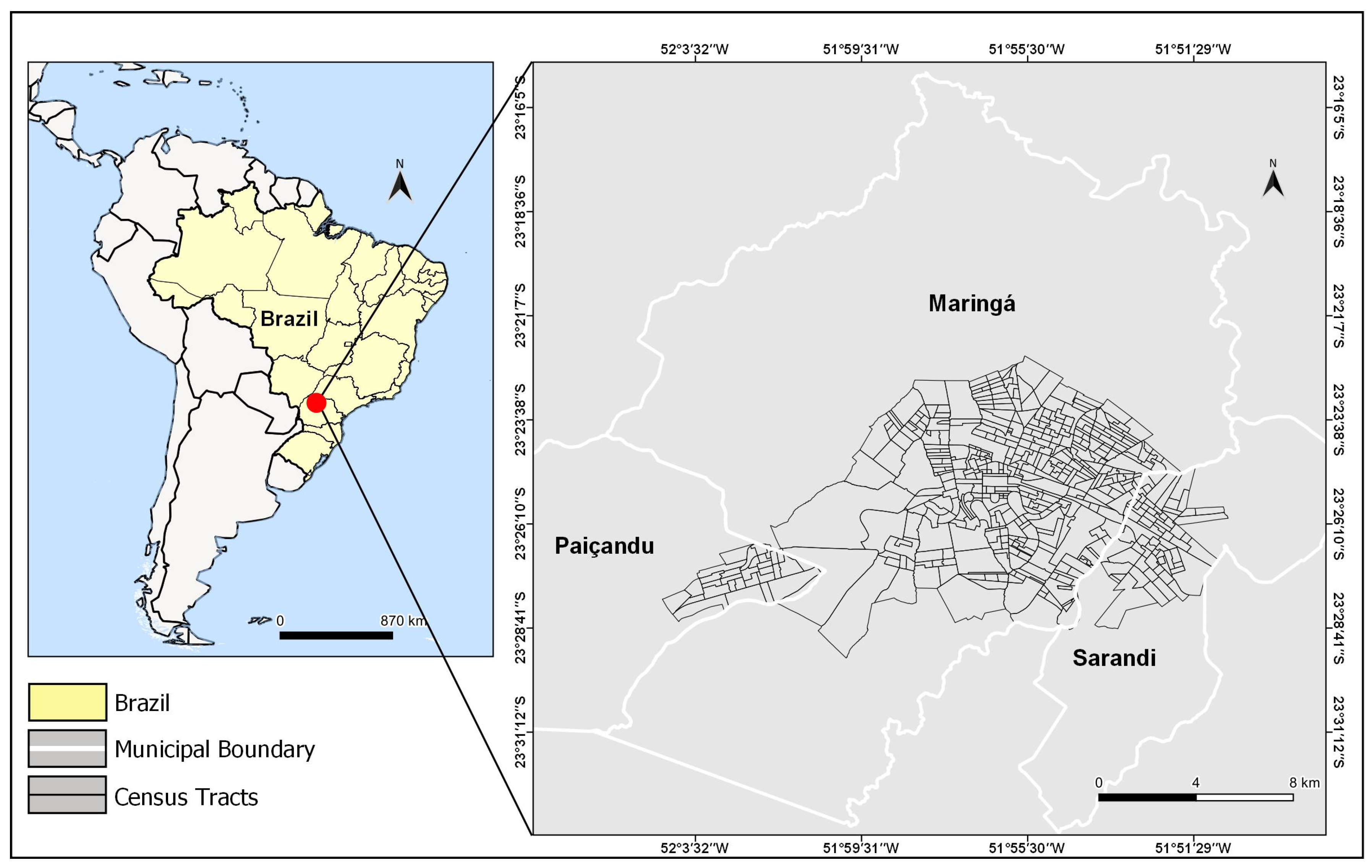
The city of Maringá is located in the northern region of the State of Paraná, Brazil (see map Figure 2). Named by the Brazilian Institute of Geography and Statistics (IBGE) [57] as the Geographic Mesoregion of the North of Paraná, Maringá is the result of the expansion of the São Paulo coffee industry [58]. Its emergence occurred in the late 1940s through the actions of Companhia Melhoramentos Norte do Paraná in the vicinity of the Rede Ferroviária Federal station, as it happened with countless other Brazilian cities [59].
IBGE data indicate that the population of Maringá has grown approximately 20% in the last 10 years, from 357,000 in 2010 [60] to 430,000 inhabitants in 2020 [61]. Together with the cities of Sarandi and Paiçandu, Maringá makes up one of the two urban conurbations of the interior of Paraná [62]. With an estimated population of 569,000 inhabitants [61], the urban conurbation of Maringá–Sarandi–Paiçandu is marked by urban inequality.
The best living conditions are located in the geometric center of the urbanized spot [63] and reflect the good social indicator performance of Maringá, which has the second highest Human Development Index and income per capita in the state [64]. The population’s living conditions worsen as we move away from the central areas [63]. Data from the 2010 Census [60] confirm this finding and show that the average nominal monthly income of Sarandi and Paiçandu was respectively 50% and 53% lower than that of Maringá.
To deepen the analysis of inequalities in the urban conurbation of Maringá–Sarandi–Paiçandu, this research uses data by census sectors, which are the smallest units of aggregation of census data in Brazil [60]. This is a geographic unit that an enumerator goes through during the collection of information from the census [60]. In the 2010 census, there were 699 urban census sectors in the urban conurbation of Maringá–Sarandi–Paiçandu, as shown in Figure 2.

5.2. Latent and Observed Variables of S-III

The variables were selected based on their theoretical and methodological relevance. From the theoretical perspective, Arretche’s work [65] shows that inequality in Brazil over the past 50 years is related to characteristics of the population (e.g., social origin, family status, race, sex, and education), the provision of public goods and services to households (e.g., garbage collection, energy networks, treated water and sewage [3,66]), and the households’ conditions (e.g., density of the household and existence of a bathroom). Among the countless variables associated with the study of social inequalities, income remains the most important [67,68]. Nevertheless, education has been listed as the variable with the greatest capacity to produce social mobility [69]. In the last decade, studies have also highlighted the close relationship between urban inequality and environmental variables. Areas with high construction density, low vegetation cover, and little street afforestation are occupied mainly by families with lower income [70], possibly due to thermal discomfort [71,72]. Peripheral areas more susceptible to environmental risks, such as landslides and floods, are also mainly occupied by lower-income families [73]. From a theoretical perspective, the variables were selected according to the Manual for the Construction of Composite Indicators [35] using the criteria of relevance, analytical strength, punctuality, and accessibility.
Given these theoretical and methodological aspects, 34 variables were selected from the three sources of information in the Demographic Census [60], thus forming the three dimensions or latent variables of intra-urban inequality. The first dimension is the socioeconomic dimension, and it gathers variables on the socioeconomic characteristics of the population. The second dimension is the neighborhood dimension, and it gathers variables on the characteristics of the surroundings of urban households. The third dimension is the household dimension, which gathers variables on the characteristics of urban households. Table 1 shows the 34 observed variables distributed in their respective dimensions or latent variables.
For the calculation of the CI, the absolute values of each variable were divided by the total number of families, households, and streets present in each census tract. The ENT_4 variable was obtained using the normalized difference vegetation index (NDVI). The NDVI identifies spectral differences between soil and vegetation, and is more sensitive to sparse vegetation. It has been widely used to estimate vegetation cover [74]. Images from the Landsat 5 satellite from 2010 were used, with a spatial resolution of 30 m and cloud coverage below 1%. All data are available in Supplementary Materials.

5.3. Model Features

The model chosen for the construction of the S-III and the analysis of relationships and effects that occur between its dimensions was the PLS-SEM. PLS-SEM is considered the most efficient model when the research is exploratory, as the sample size may be smaller than in CB-SEM and the data distribution does not need to be Gaussian [50]. In addition, PLS-SEM makes it possible to keep a greater number of variables in each construct [12,49]. The relationship between latent and observed variables in the model was classified as reflexive. This is because changes in latent variables influence the measurement of the observed variables [52]. The following effects of the latent variables were considered: socioeconomic inequality influencing household inequality; households inequality influencing neighborhood inequality; and urban inequality being influenced by socioeconomic, household, and neighborhood inequalities.
The two-stage model was created using the SmartPLS Software [75]. The first stage is associated with the modeling of the first-order structure, in which the observed variables are selected. The criterion for selecting an observed variable is the loading factor [12]. The factor loading criterion threshold is 0.70 [49]. This implies that the greater part of the observed variable variance is captured by the latent variables of the first-order structure, namely neighborhood inequality, socioeconomic inequality, and household inequality. In PLS-SEM, these constructs are associated to the latent variables that quantitatively represent the dimensions of long-distance inequality. In the second stage, the latent variables obtained in the first-order structure are used to establish the CIs of the second-order structure, the latent variable S-III.

5.4. Parameters for S-III Analysis

The parameters used for S-III analysis are: (a) the outer weights and outer loadings, which respectively reflect the relative importance of variables in the construct and the absolute contribution of variables in the construct; (b) the path coefficient, which shows the standardized direct and indirect effects between model variables; (c) the average variance extracted (AVE), which reflects which proportion of the information contained in the observed variables is captured/explained by the latent variable; (d) the convergent validity, which verifies the reliability of the constructs, that is, whether the observed variables of a construct produce similar outer loadings, and which can be tested for internal validity or composite reliability; (e) the discriminant validity, which tests whether a latent variable differs from the others; and (f) the coefficient of determination R 2 , which expresses the amount of variance in the data that is explained by the model [12,49].

5.5. Validation of PLS-SEM Parameters

The S-III was validated through six tests: convergent validity, internal consistency, composite reliability, discriminant validity, internal validity of the model, and overall validity of the model.
First, Fornell and Larcker [76] suggest using AVE as a convergent validity criterion for PLS-SEM. To the authors, convergent validity is acceptable when the stroke is equal to or greater than 0.5, and when the latent variable explains, on average, more than half of the variance of the variables observed. Second, the internal consistency of the PLS-SEM is tested using Cronbach’s alpha coefficient (CA, [41]) and, third, the reliability is composed using Dillon–Goldstein’s Rho value [40]. Hair et al. [12] suggest that the values of the internal consistency of exploratory studies be higher than 0.6 and the values of composite reliability be higher than 0.7. Fourth, the discriminating validity of PLS-SEM can be obtained in three ways. According to Fornell and Larcker [76], the AVE of each latent variable must be greater than all the squared correlations of this variable with the others. According to the cross-loading criterion, the factor load of the variables of a construct must be greater than its factor loading in other constructs [10]. According to the heterotrait–monotrait (HTMT) ratio of correlation criteria, the result of the test must be less than 0.9, which makes it the most conservative test, as it reaches the lowest specificity rates of all simulation conditions [77]. Fifth, the internal validation of PLS-SEM is done by reading the significance and strength of relationships. Student’s t-test is used to verify the significance of relationships and must be greater than or equal to 1.96 [12]. The coefficient of determination R 2 , used to measure the strength of relationships, can be rated as substantial (R 2 > 0.67), moderate (0.67 < R 2 > 0.33), or weak (R 2 < 0.33) [10]. Sixth, the global validity criteria of the PLS-SEM model are in their initial research stage, and the threshold and critical values are not fully understood or established, making them of little use for PLS-SEM [12], so they were not considered.

5.6. Visualization of the S-III PLS-SEM

Four maps were created to visualize the PLS-SEM of the S-III. The maps were created using the QGIS software with Datum SIRGAS 2000 and Projection UTM 23 South. The maps were prepared from the normalized scores of each indicator, composed of four classes: high social exclusion, medium social exclusion, low social exclusion, and social inclusion. The upper limits of the classes were, respectively: 0.25, 0.50, 0.75, and 1.00.

6. Results and Discussions

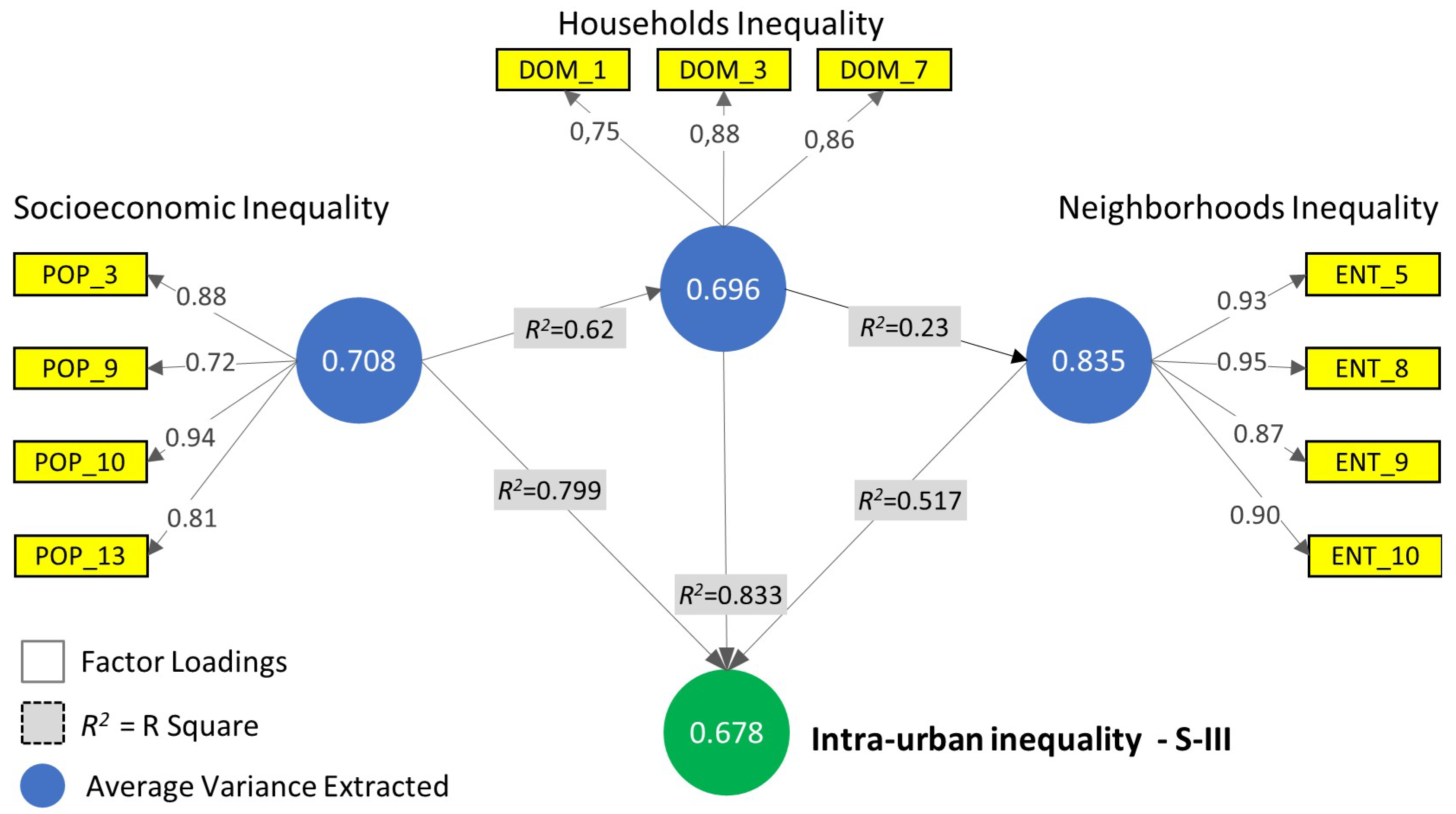
For the definition of the first-order structure that determines the creation of the latent variables representing the underlying dimensions of intra-urban inequality, 11 variables that exceeded the loading threshold of 0.70 [12] were selected. This threshold means that the latent variable explains at least 50% of the variance of the observed variable [49]. Neighborhood inequality comprised the following observed variables: streets without paving (ENT_5); wireless locations (ENT_8); public places without manholes (ENT_9); and streets without sidewalks (ENT_10). Socioeconomic inequality was made up of the following observed variables: number of people of brown color/race (POP_3); number of heads of household with income below or equal to 2 minimum wages (POP_9); number of heads of households with income above 20 minimum wages (POP_10); and number of illiterate heads of household (POP_13). Finally, households inequality comprised the following observed variables: average household income (DOM_1); households with four bathrooms or more (DOM_3); and inadequate housing (DOM_7). These three constructs make up the second-order urban inequality structure, the S-III. The results of the reliability and validity tests of the first- and second-order structures are shown in Table 2.
As noted, all constructs tested internal consistency, composite reliability, and convergent validity above critical reference values. The discriminating validity of the three constructs that make up the S-III presents conflicting results. According to Fornell and Larcker [76], as seen in Table 3, the AVE of each latent variable is greater than all the squared correlations of this latent variable with the others.
The HTMT criterion states that discriminant validity occurs when the test result is less than 0.90. Considering that the HTMT values of the neighborhood inequality and socioeconomic inequality constructs were 0.466 and 0.551 for the neighborhood inequality and household inequality constructs, it can be said that these constructs are different. The HTMT of 0.904 does not allow the affirmation that the socioeconomic inequality and household inequality constructs are different. The explanation for the failure in this test is obtained by the criterion of cross-loading [10]. By this criterion, it is observed in Table 4 that the outer loading of the average household income variable (DOM_1) in red is greater in the socioeconomic inequality construct than in its origin construct, household inequality.
Although the results of the discriminant validity are divergent, we highlight in the words of Henseler et al. [77] (p. 131) that “a failure to establish the discriminating validity between two constructs does not imply that the concepts are identical”, especially when the research provides support for this differentiation. This differentiation exists if the IBGE [60] classifies the average household income as household data, even if such income is associated with the families’ income. Finally, the PLS-SEM internal validity tests the relationship between the constructs that form the S-III reflecting urban inequality. The results of this test are illustrated in Figure 3, which also shows the factor loadings of the observed variables of each latent variable and the AVE of the latent variables.
It can be seen in Figure 3 that all relationships exceeded the critical significance value: t-test > 1.96 [12]. However, the strength of these relationships is not homogeneous. In particular: (i) Socioeconomic inequality is moderately related to household inequality (0.67 > R 2 > 0.33); (ii) households inequality is weakly related to neighborhood inequality (R 2 > 0.33); (iii) neighborhood inequality is moderately related to urban inequality (0.67 > R 2 > 0.33), which, in turn, is substantially related to socioeconomic inequality and household inequality (R 2 > 0.67). From the presence of these statistically significant relationships, it is possible to know what the direct and indirect effects between the latent variables that form the S-III are. Table 5 shows these direct and indirect effects.
The results presented in Table 5 show that socioeconomic inequality influences household inequality, and that household inequality influences neighborhood inequality. First, changes of one standard deviation in socioeconomic inequality influence household inequality by 0.785 standard deviations. Second, changes of one standard deviation in household inequality influence neighborhood inequality by 0.482 standard deviations. Table 5 also shows that changes of one standard deviation in socioeconomic inequality influence neighborhood inequality by 0.378 standard deviations. It is noteworthy that this last relationship is the influence of an indirect effect. In the model presented in Figure 3, it can be seen that there is no significant relationship between socioeconomic inequality and neighborhood inequality. The explanation for the occurrence of this indirect effect is in the following sequence of significant relationships: socioeconomic inequality -> household inequality -> neighborhood inequality.
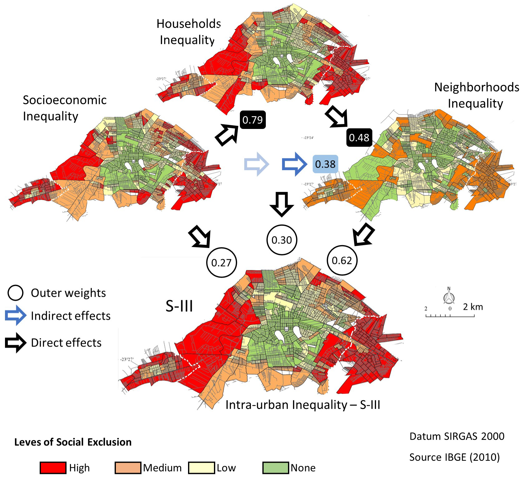
The internal validity test shows that the relationships between the underlying dimensions of intra-urban inequality are statistically valid. In turn, the coefficients of determination indicate that the chances of these relationships occurring as they were estimated vary between R2 = 0.23 and R2 = 0.83. It is, therefore, necessary to add the relative importance of each underlying dimension of intra-urban inequality in the S-III. This relative importance is indicated by the outer weights [12] of 0.27, 0.30, and 0.62 of the socioeconomic, household, and neighborhood dimensions, respectively, in the S-III construct of intra-urban inequality. The relative importance of each underlying dimension of intra-urban inequality in S-III can be seen in the circles of Figure 4. The indirect effects between the underlying dimensions can also be observed beside the black and blue arrows.
As seen in Figure 4, neighborhood inequality is influenced directly by household inequality and indirectly by socioeconomic inequality. These influences are reflected both in the relative importance measured by the outer weights (OW) and in the absolute contribution measured by the outer loadings (OL) of the neighborhood inequality latent variable in the intra-urban inequality construct. Table 6 shows the OW and OL of the underlying dimensions of intra-urban inequality in the S-III construct.
The results in Table 6 indicate that socioeconomic and household inequalities have less relative and absolute importance in the intra-urban inequality S-III construct than neighborhood inequality. The OW of 0.27 and 0.30 and the OL of 0.77 and 0.81 of socioeconomic and household inequalities are less than the OW of 0.62 and the 0.88 OL of neighborhood inequality. These results suggest that neighborhood inequality is the most important dimension in the formation of the intra-urban inequality S-III construct. Proportionally, neighborhood inequality, household inequality, and socioeconomic inequality contribute 52%, 25%, and 23% to S-III, respectively.

Contributions

Determining which dimensions and variables to use in the study of inequalities is always a hard task because of the availability and quality of the data concerning the breakdown, coverage, detailing, periodicity, and reliability. Given the availability, it is necessary, based on the conceptualization of the phenomenon, to define which data to select to develop indicators that are both pertinent and economical. The definition of which data to use is not a simple task, because in each socio-spatial context, there are specific combinations that more accurately reflect the analyzed phenomenon, which is, in this case, inequality.
In this sense, the present work contributes to: (i) the definition of, based on a significant number of data, that which most consistently represents each dimension of the phenomenon; (ii) the definition of which of these dimensions contributes most to the final indicator—in this case, the urban inequality indicator; and (iii) showing the levels of precariousness that together help to identify urban inequalities.
For the case of the urban conurbation of Maringá–Sarandi–Paiçandu, it has as a practical contribution the conclusion that the variables related to the basic urban infrastructure, such as paving of roads, rain galleries, or sidewalks, highly discriminate against the most vulnerable areas of the city, expressing striking intra-urban inequalities. This shows that the inequality to which citizens are subject is not linked to income level, but also to the conditions in the place where they live. In summary, the place of residence and its characteristics weigh heavily in the creation, conservation, and deepening of social inequalities that are also territorial. Often, it weighs heavily on the perpetuation of social disadvantages across generations, as the studies by Stiglitz [78] and Deaton [79] have pointed out.
These analyses allow us to conclude that with the urban conurbation of Maringá–Sarandi–Paiçandu, the urban spaces with precarious infrastructure are representative icons of intra-urban inequality and denote precariousness in the living standards of families closely related to levels of education and income, as well as their color/race.

7. Conclusions

This work used PLS-SEM to capture the direct and indirect effects of the underlying dimensions of urban inequality in a summary indicator: neighborhood inequality, socioeconomic inequality, and household inequality. Beyond quantifying a multidimensional phenomenon, this research shows how to perform a theorized measurement of urban inequality. From this measurement, it is possible to identify which dimensions most influence the others, and which dimensions have greater weight in the measurement of urban inequality. This identification makes it possible, for example, to establish tax zones for the taxation of urban property, to develop investment plans in urban infrastructure, or to prioritize areas for implementing public policies aimed at reducing inequality.
With the urban conurbation of Maringá–Sarandi–Paiçandu, socioeconomic inequality is the dimension that most influences the others, while neighborhood inequality has greater weight in urban inequality. In this sense, improvements in the socioeconomic conditions of less favored regions, for example, from the exemption from property tax, can encourage families to invest in the conditions of their homes. For example, improvements in the conditions of the neighborhood in urban infrastructure have significant weight in reducing the urban inequality of the urban conurbation of Maringá–Sarandi–Paiçandu.
Although the PLS-SEM offers different spectra of analysis to support inequality reduction policies, it is necessary to remember that statistical methods of this nature are not immune to errors and distortions because the model’s responses do not perfectly represent the phenomenon or interrelationships. For this, the AVE and correlation coefficients should be equal to 1. In addition, because the answers found in the model did not occur in all areas, atypical observations show that the model does not apply to the entire city (see Appendix A). A final limitation can be attributed to the frequency at which census data are updated. In Brazil, as in many countries, these census data are updated every ten years [60]. As a result, the indicators built tend not to represent a present reality. Therefore, it is a challenge for future research to develop methodologies that make it possible to update census data and, based on these data, develop longitudinal analyses of multidimensional phenomena.
Supplementary Materials

The data used in this research are available at http://dx.doi.org/10.17632/8j836n4bys.3.

Author Contributions

Conceptualization, M.P.L. and O.d.S.M.; Data curation, P.E.; Formal analysis, M.P.L., R.d.M.L., A.M.C.M., and P.E.; Funding acquisition, O.d.S.M. and S.L.; Investigation, O.d.S.M.; Methodology, M.P.L., S.L., and A.M.C.M.; Project administration, P.B.; Supervision, P.B.; Validation, P.E.; Writing—original draft, M.P.L., O.d.S.M., and R.d.M.L.; Writing—review and editing, S.L., A.M.C.M., P.B., and P.E. All authors have read and agreed to the published version of the manuscript.

Funding

This research was supported by the National Scientific and Technological Development of Brazil (CNPq) [grant numbers: 423443/2016-0 and 311032/2016-8] and Coordination for the Improvement of Personnel in Higher Education—Brasil (CAPES) [Finance Code 0001].

Conflicts of Interest

The authors declare no conflict of interest. The funders had no role in the design of the study; in the collection, analyses, or interpretation of data; in the writing of the manuscript, or in the decision to publish the results.

Appendix A. Considerations on Atypical Observations that Occurred in the Model

The interrelationships between the latent variables of some areas of the urban conurbation of Maringá–Sarandi–Paiçandu shown in Table A1 do not correspond to what was found in the PLS-SEM, as shown in Table A2.
Table A1. Coefficients for determination of the PLS-SEM model for the urban conurbation of Maringá–Sarandi–Paiçandu from atypical observations.
Inequality IndicatorNeighborhoodSocioeconomicHouseholdUrban
Neighborhood1.00
Socioeconomic0.391.00
Household−0.09−0.281.00
Urban0.720.90−0.071.00
Table A2. Coefficients for determination of the PLS-SEM model for the urban conurbation of Maringá–Sarandi–Paiçandu.
Inequality IndicatorNeighborhoodSocioeconomicHouseholdUrban
Neighborhood1.00
Socioeconomic0.191.00
Household0.230.621.00
Urban0.780.600.661.00
These cases exemplify situations in which the S-III does not adequately represent the reality of urban inequality. The interrelationships found in the tables that presented the most dissimilar results were: (i) household inequality and socioeconomic inequality, and (ii) urban inequality and household inequality. In the S-III, household inequality is positively and significantly influenced by socioeconomic inequality, and urban inequality is positively and significantly influenced by household inequality. In the atypical areas, the interrelationship between the constructs is negative and not significant. The PLS-SEM does not present consistent results for all areas of the city.
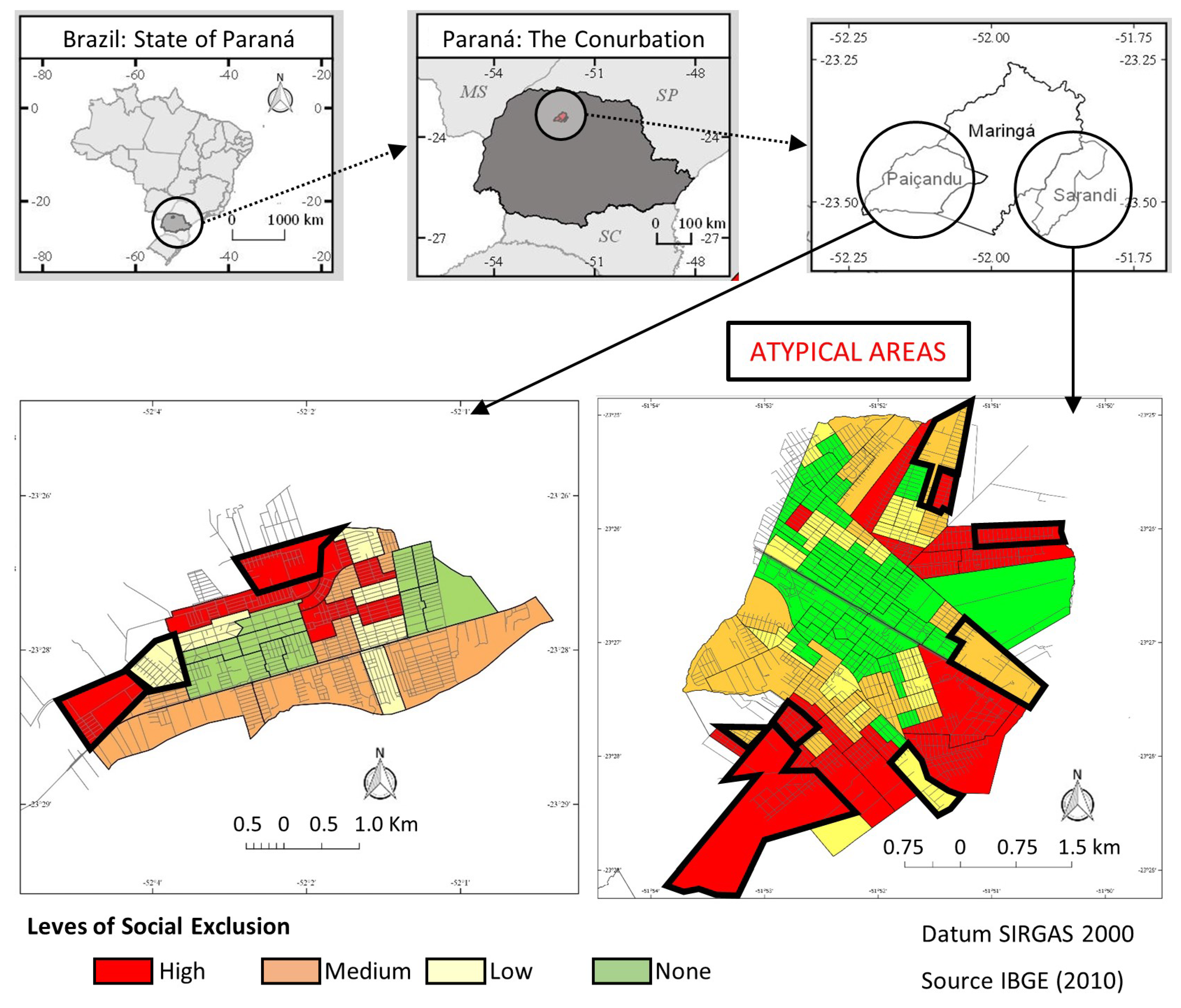
Although the percentage of atypical cases is small, only 2.28% of census tracts, it is possible to conclude that: (i) All atypical areas are peripheral areas of Sarandi and Paiçandu, which are the cities contributing to Maringá, but which are peripheries; (ii) three atypical areas are in Paiçandu, and the other eight areas are in Sarandi, also with peripheral locations (see Figure 1); (iii) all atypical areas are urban expansion areas. They may have a good home infrastructure, but might not be connected to networks (water and sewage); as they were urbanization areas in 2010, they may have little afforestation and fragile infrastructures, such as sidewalks, ramps, and garbage collection. Therefore, it is natural that the largest number of atypical areas is in Sarandi. Almost the whole city has problems with urban infrastructure, despite having axes and urbanization areas that make the structures of the homes good, despite not being connected to the sewage network, for example. This also happens with Paiçandu, although to a lesser extent. As represented by Figure 1, it is observed that the atypical areas are mostly classified as having high social exclusion.
Some other data about the atypical areas:
  • Together, the atypical areas have 27,568 inhabitants in 8278 households.
  • Only two atypical areas, both in Sarandi, have one head of households with an income above 20 minimum wages
  • Few households are connected to the sewage network (1.06%), but a significant portion are connected to the water network (48.78%).
  • Few households are considered inadequate housing (0.06%).
  • Few households have open sewage (average 0.64) (although most are not connected to the sewer network).
  • On average, 50% of the households have no afforestation.
  • On average, 45% of the garbage is accumulated in the street.
Figure A1. Map of atypical areas.
Sustainability 12 08610 g0a1

References

  1. Cataldo, R.; Grassia, M.G.; Lauro, N.C.; Marino, M. Developments in Higher-Order PLS-PM for the building of a system of Composite Indicators. Qual. Quant. 2017, 51, 657–674. [Google Scholar] [CrossRef]
  2. El Gibari, S.; Gómez, T.; Ruiz, F. Building composite indicators using multicriteria methods: A review. J. Bus. Econ. 2019, 89, 1–24. [Google Scholar] [CrossRef]
  3. Libório, M.P.; Laudares, S.; Abreu, J.F.d.; Ekel, P.Y.; Bernardes, P. Property tax: Dealing spatially with economic, social, and political challenges. Urbe. Revista Brasileira de Gestão Urbana 2020, 12. [Google Scholar] [CrossRef]
  4. Drachler, M.d.L.; Lobato, M.A.d.O.; Lermen, J.I.; Fagundes, S.; Ferla, A.A.; Drachler, C.W.; Teixeira, L.B.; Leite, J.C.d.C. Desenvolvimento e validação de um índice de vulnerabilidade social aplicado a políticas públicas do SUS. Ciência Saúde Coletiva 2014, 19, 3849–3858. [Google Scholar] [CrossRef] [PubMed] [Green Version]
  5. Bellini, J.H.; Stephan, Í.I.C.; Gleriani, J.M. A desigualdade ambiental em Rio das Ostras-RJ, Brasil. Raega-O Espaço Geográfico em Análise 2016, 38, 82–106. [Google Scholar] [CrossRef] [Green Version]
  6. Arranz, J.M.; García-Serrano, C.; Hernanz, V. Employment quality: Are there differences by types of contract? Soc. Indic. Res. 2018, 137, 203–230. [Google Scholar] [CrossRef]
  7. Yu, D.; Fang, C.; Xue, D.; Yin, J. Assessing urban public safety via indicator-based evaluating method: A systemic view of Shanghai. Soc. Indic. Res. 2014, 117, 89–104. [Google Scholar] [CrossRef]
  8. Silva, D.B.L.; Rosa, E. Índice de Carência e Vulnerabilidade Municipal–ICV-M: Análise Crítica e Metodologica. Rev. Gest. Secretariado 2017, 8, 201–223. [Google Scholar]
  9. Tarka, P. An overview of structural equation modeling: Its beginnings, historical development, usefulness and controversies in the social sciences. Qual. Quant. 2018, 52, 313–354. [Google Scholar] [CrossRef] [Green Version]
  10. Chin, W.W. The partial least squares approach to structural equation modeling. Mod. Methods Bus. Res. 1998, 295, 295–336. [Google Scholar]
  11. Hair, J.F.; Ringle, C.M.; Sarstedt, M. Partial least squares structural equation modeling: Rigorous applications, better results and higher acceptance. Long Range Plan. 2013, 46, 1–12. [Google Scholar] [CrossRef]
  12. Hair, J.F., Jr.; Hult, G.T.M.; Ringle, C.; Sarstedt, M. A Primer on Partial Least Squares Structural Equation Modeling (PLS-SEM); Sage Publications: Thousand Oaks, CA, USA, 2016. [Google Scholar]
  13. Holzer, H.J. Informal job search and black youth unemployment. Am. Econ. Rev. 1987, 77, 446–452. [Google Scholar]
  14. Holzer, H.J. The spatial mismatch hypothesis: What has the evidence shown? Urban Stud. 1991, 28, 105–122. [Google Scholar] [CrossRef]
  15. Harvey, D. Social justice, postmodernism and the city. Int. J. Urban Reg. Re. 1992, 16, 588–601. [Google Scholar] [CrossRef]
  16. Harvey, D. Social Justice and the City; University of Georgia Press: Athens, GA, USA, 2010; Volume 1. [Google Scholar]
  17. Clark, W.W.A.; Dieleman, F.M. Households and Housing: Choice and Outcomes in the Housing Market; Transaction Publishers: Piscataway, NJ, USA, 1996. [Google Scholar]
  18. Massey, D.S. American apartheid: Segregation and the making of the underclass. Am. J. Sociol. 1990, 96, 329–357. [Google Scholar] [CrossRef]
  19. Sampson, R.J.; Raudenbush, S.W.; Earls, F. Neighborhoods and violent crime: A multilevel study of collective efficacy. Science 1997, 277, 918–924. [Google Scholar] [CrossRef]
  20. Sampson, R.J.; Laub, J.H. Crime in the Making: Pathways and Turning Points through Life; Harvard University Press: Cambridge, MA, USA, 1995. [Google Scholar]
  21. Wilson, W.J. The Truly Disadvantaged: The Inner City, the Underclass, and Public Policy; University of Chicago Press: Chicago, IL, USA, 2012. [Google Scholar]
  22. Boyack, K.W.; Klavans, R. Co-citation analysis, bibliographic coupling, and direct citation: Which citation approach represents the research front most accurately? J. Am. Soc. Inf. Sci. Technol. 2010, 61, 2389–2404. [Google Scholar] [CrossRef]
  23. Small, H. Co-citation in the scientific literature: A new measure of the relationship between two documents. J. Am. Soc. Inf. Sci. Technol. 1973, 24, 265–269. [Google Scholar] [CrossRef]
  24. Van Eck, N.J.; Waltman, L. VOSviewer manual. Leiden Univ. Leiden 2013, 1, 1–53. [Google Scholar]
  25. Massey, D.; Denton, N.A. American Apartheid: Segregation and the Making of the Underclass; Harvard University Press: Cambridge, MA, USA, 1993. [Google Scholar]
  26. Farley, R.; Frey, W.H. Changes in the segregation of whites from blacks during the 1980s: Small steps toward a more integrated society. Am. Sociol. Rev. 1994, 59, 23–45. [Google Scholar] [CrossRef]
  27. Noble, M.; Barnes, H.; Wright, G.; Roberts, B. Small area indices of multiple deprivation in South Africa. Soc. Indic. Res. 2010, 95, 281. [Google Scholar] [CrossRef]
  28. Rubio, C.; Rubio, M.C.; Abraham, E. Poverty Assessment in Degraded Rural Drylands in the Monte Desert, Argentina. An Evaluation Using GIS and Multi-criteria Decision Analysis. Soc. Indic. Res. 2018, 137, 579–603. [Google Scholar] [CrossRef]
  29. Luh, J.; Baum, R.; Bartram, J. Equity in water and sanitation: Developing an index to measure progressive realization of the human right. Int. J. Hyg. Environ. Health 2013, 216, 662–671. [Google Scholar] [CrossRef] [PubMed]
  30. Baquero, O.F.; Gallego-Ayala, J.; Giné-Garriga, R.; de Palencia, A.J.F.; Pérez-Foguet, A. The influence of the human rights to water and sanitation normative content in measuring the level of service. Soc. Indic. Res. 2017, 133, 763–786. [Google Scholar] [CrossRef] [Green Version]
  31. Lauro, N.C.; Grassia, M.G.; Cataldo, R. Model based composite indicators: New developments in partial least squares-path modeling for the building of different types of composite indicators. Soc. Indic. Res. 2018, 135, 421–455. [Google Scholar] [CrossRef]
  32. Zannella, M.; De Rose, A. Stability and change in family time transfers and workload inequality in Italian couples. Demogr. Res. 2019, 40, 49–60. [Google Scholar] [CrossRef] [Green Version]
  33. Saisana, M.; Tarantola, S. State-of-the-Art Report on Current Methodologies and Practices for Composite Indicator Development; Citeseer: Ispra (VA), Italy, 2002; Volume 214. [Google Scholar]
  34. Nardo, M.; Saisana, M.; Saltelli, A.; Tarantola, S. Tools for composite indicators building. Eur. Com. Ispra 2005, 15, 19–20. [Google Scholar]
  35. European Commission, Joint Research Centre and OECD; Nardo, M.; Saisana, M.; Saltelli, A.; Tarantola, S.; Hoffman, A.; Giovannini, E. Handbook on Constructing Composite Indicators: Methodology and User Guide; OECD Publishing: Paris, France, 2008. [Google Scholar]
  36. Becker, W.; Saisana, M.; Paruolo, P.; Vandecasteele, I. Weights and importance in composite indicators: Closing the gap. Ecol. Indic. 2017, 80, 12–22. [Google Scholar] [CrossRef] [PubMed]
  37. Greco, S.; Ishizaka, A.; Tasiou, M.; Torrisi, G. On the methodological framework of composite indices: A review of the issues of weighting, aggregation, and robustness. Soc. Indic. Res. 2019, 141, 61–94. [Google Scholar] [CrossRef] [Green Version]
  38. Kuc-Czarnecka, M.; Piano, S.L.; Saltelli, A. Quantitative storytelling in the making of a composite indicator. Soc. Indic. Res. 2020, 149, 775–802. [Google Scholar] [CrossRef] [Green Version]
  39. Saaty, T.L. What is the analytic hierarchy process? In Mathematical Models for Decision Support; Springer: Berlin/Heidelberg, Germany, 1988; pp. 109–121. [Google Scholar]
  40. Dillon, W.R.; Goldstein, M. Multivariate Analysis Methods and Applications; Wiley: Hoboken, NJ, USA, 1984. [Google Scholar]
  41. Cronbach, L.J. Coefficient alpha and the internal structure of tests. Psychometrika 1951, 16, 297–334. [Google Scholar] [CrossRef] [Green Version]
  42. Pearson, K. LIII. On lines and planes of closest fit to systems of points in space. Lond. Edinb. Dublin Philos. Mag. J. Sci. 1901, 2, 559–572. [Google Scholar] [CrossRef] [Green Version]
  43. Adachi, K. Principal Component Analysis Versus Factor Analysis. In Matrix-Based Introduction to Multivariate Data Analysis; Springer: Berlin/Heidelberg, Germany, 2020; pp. 297–310. [Google Scholar]
  44. Greenacre, M.J. Theory and Applications of Correspondence Analysis; Academic Press: London, UK, 1984. [Google Scholar]
  45. Greenacre, M. Correspondence Analysis in Practice; CRC Press: Boca Raton, FL, USA, 2017. [Google Scholar]
  46. Šlachtová, H.; Tomášková, H.; Šplíchalová, A.; Polaufová, P.; Fejtková, P. Czech socio-economic deprivation index and its correlation with mortality data. Int. J. Public Health 2009, 54, 267–273. [Google Scholar] [CrossRef]
  47. Jöreskog, K. Analysis of covariance structures. In Multivariate Analysis, III; Krishnaiah, P.R., Ed.; Academic Press: New York, NY, USA, 1973; pp. 263–285. [Google Scholar]
  48. Hair, J.F.; Ringle, C.M.; Sarstedt, M. PLS-SEM: Indeed a silver bullet. J. Mark. Theory Pract. 2011, 19, 139–152. [Google Scholar] [CrossRef]
  49. Hair, J.F.; Risher, J.J.; Sarstedt, M.; Ringle, C.M. When to use and how to report the results of PLS-SEM. Eur. Bus. Rev. 2019, 31. [Google Scholar] [CrossRef]
  50. Astrachan, C.B.; Patel, V.K.; Wanzenried, G. A comparative study of CB-SEM and PLS-SEM for theory development in family firm research. J. Fam. Bus. Strateg. 2014, 5, 116–128. [Google Scholar] [CrossRef]
  51. Jarvis, C.B.; MacKenzie, S.B.; Podsakoff, P.M. A critical review of construct indicators and measurement model misspecification in marketing and consumer research. J. Consum. Res. 2003, 30, 199–218. [Google Scholar] [CrossRef]
  52. Petter, S.; Straub, D.; Rai, A. Specifying formative constructs in information systems research. MIS Q. 2007, 31, 623–656. [Google Scholar] [CrossRef] [Green Version]
  53. Park, H.; Fan, P.; John, R.; Chen, J. Urbanization on the Mongolian Plateau after economic reform: Changes and causes. Appl. Geogr. 2017, 86, 118–127. [Google Scholar] [CrossRef]
  54. Boccuzzo, G.; Fordellone, M. Comments about the Use of PLS Path Modeling in Building a Job Quality Composite Indicator. Working Paper Series No 2, University of Padua, Department of Statistical Sciences 2015. Available online: http://paduaresearch.cab.unipd.it/8841/ (accessed on 16 October 2020).
  55. Davino, C.; Dolce, P.; Taralli, S.; Vinzi, V.E. A quantile composite-indicator approach for the measurement of equitable and sustainable well-being: A case study of the italian provinces. Soc. Indic. Res. 2018, 136, 999–1029. [Google Scholar] [CrossRef]
  56. Buil-Gil, D.; Medina, J.; Shlomo, N. The geographies of perceived neighbourhood disorder. A small area estimation approach. Appl. Geogr. 2019, 109, 102037. [Google Scholar] [CrossRef] [Green Version]
  57. IBGE. Divisão Regional do Brasil em Mesorregiões e Microrregiões Geográficas. v. 1; Brazilian Institute of Geography and Statistics: Rio de Janeiro, Brazil, 1990.
  58. Martins, R. História do Paraná; Prefeitura Municipal de Curitiba: Curitiba, Brazil, 1995.
  59. Priori, A.; Pomari, L.R.; Amâncio, S.M.; Ipólito, V.K. História do Paraná: Séculos XIX e XX; EDUEM: Maringa, Brazil, 2012. [Google Scholar]
  60. IBGE. Population Census 2010. 2010. Available online: https://censo2010.ibge.gov.br/resultados.html (accessed on 16 October 2020).
  61. IBGE. Population Estimates. 2020. Available online: https://www.ibge.gov.br/estatisticas/sociais/populacao/9103-estimativas-de-populacao.html (accessed on 16 October 2020).
  62. IBGE. Arranjos Populacionais e Concentrações Urbanas no Brasil, 2nd ed.; IBGE: Rio de Janeiro, Brazil, 2016; ISBN 978-85-240-4406-9.
  63. IBGE. Tipologia Intraurbana: Espaços de Diferenciação Socioeconômica nas Concentrações Urbanas do Brasil; IBGE: Rio de Janeiro, Brazil, 2017; ISBN 978-85-240-4429-8.
  64. UNDP—United Nations Development Programme. Desenvolvimento Humano Nas Macrorregiões Brasileiras; UNP: Brasília, Brazil, 2016; ISBN 978-85-88201-31-6. [Google Scholar]
  65. Arretche, M. Paths of Inequality in Brazil: A Half-Century of Changes; Springer: Berlin/Heidelberg, Germany, 2018. [Google Scholar]
  66. Arretche, M. The Geography of Access to Basic Services in Brazil. In Paths of Inequality in Brazil; Springer: Berlin/Heidelberg, Germany, 2019; pp. 137–161. [Google Scholar]
  67. Piketty, T. The Economics of Inequality; Harvard University Press: Cambridge, MA, USA, 2015. [Google Scholar]
  68. Libório, M.; Martinuci, O.; Bernardes, P.; Ekel, P. Medidas e escalas de desigualdade de renda em perspectiva. GOT Rev. Geogr. Ordenam. Território 2018, 287–314. [Google Scholar] [CrossRef]
  69. Menezes Filho, N.; Kirschbaum, C. Education and Inequality in Brazil. In Paths of Inequality in Brazil; Springer: Berlin/Heidelberg, Germany, 2019; pp. 69–88. [Google Scholar]
  70. Farias, F.O.; Bargos, D.C.; Matias, L.F. Aplicação de geotecnologias no estudo da relação entre a valorização da terra urbana e a presença de áreas verdes na cidade de Paulínia (SP). Rev. Bras. Cartogr. 2016, 68, 275–287. [Google Scholar]
  71. Amorim, M.C.D.C.T.; Monteiro, A. As temperaturas intraurbanas: Exemplos do Brasil e de Portugal. Confins. Rev. Franco-Brés. Géogr./Rev. Franco-Bras. Geogr. 2011, 13. [Google Scholar] [CrossRef]
  72. Santos Cardoso, R.; Amorim, M.C.d.C.T. Análise do clima urbano a partir da segregação socioespacial e socioambiental em Presidente Prudente-SP, Brasil. GEOSABERES Rev. Estudos Geoeduc. 2015, 6, 122–136. [Google Scholar]
  73. Carreço, H.; Castiglioni, A.H. Analysis of socio-environmental vulnerability in the municipality of Vitória-ES, with the support of a free GIS. Caderno Geogr. 2018, 28, 1076–1102. [Google Scholar] [CrossRef] [Green Version]
  74. Pettorelli, N. The Normalized Difference Vegetation Index; Oxford University Press: Oxford, UK, 2013. [Google Scholar]
  75. Sarstedt, M.; Cheah, J.H. Partial least squares structural equation modeling using SmartPLS: A software review. J. Mark. Anal. 2019, 7, 196–202. [Google Scholar] [CrossRef]
  76. Fornell, C.; Larcker, D.F. Structural Equation Models with Unobservable Variables and Measurement Error: Algebra and Statistics. J. Mark. Res. 1981, 18, 382–388. [Google Scholar] [CrossRef]
  77. Henseler, J.; Ringle, C.M.; Sarstedt, M. A new criterion for assessing discriminant validity in variance-based structural equation modeling. J. Acad. Mark. Sci. 2015, 43, 115–135. [Google Scholar] [CrossRef] [Green Version]
  78. Stiglitz, J.E. The Price of Inequality: How Today’s Divided Society Endangers Our Future; WW Norton & Company: New York, NY, USA, 2012. [Google Scholar]
  79. Deaton, A. The Great Escape: Health, Wealth, and the Origins of Inequality; Princeton University Press: Princeton, NJ, USA, 2013. [Google Scholar]
Figure 1. Research fronts on urban inequality/co-citation analysis.
Sustainability 12 08610 g001
Figure 2. Location map of the Maringá–Sarandi–Paiçandu urban conurbation, Paraná State, Brazil.
Sustainability 12 08610 g002
Figure 3. S-III Partial Least Square Structural Equation Mdeling (PLS-SEM): observed variables, latent variables, and relationships.
Sustainability 12 08610 g003
Figure 4. Influences between dimensions of intra-urban inequality and their relative importance in S-III.
Sustainability 12 08610 g004
Table 1. Observed variables and Structured Intra-urban Inequality Indicator (S-III) constructs.
DimensionCodeDescription of Observed Variables
SocioeconomicPOP_1Number of people of color/race: Black
inequalityPOP_2Number of people of color/race: Indigenous
POP_3Number of people of color/race: Brown
POP_4Number of people per household (density of household)
POP_5Number of heads of households aged 10 to 19 years
POP_6Number of dependents per head of household
POP_7Number of people up to one year old
POP_8Number of heads of households without income
POP_9Number of heads of households with income above 20 minimum wages
POP_10Number of heads of household with income below or equal to 2 minimum wages
POP_11Number of female heads of households
POP_12Number of illiterate children between 10 and 14 years old
POP_13Number of illiterate heads of household
NeighborhoodENT_1Street with accumulated garbage
inequalityENT_2Street without afforestation
ENT_3Street with open sewer
ENT_4Street with vegetation cover
ENT_5Street without paving
ENT_6Street without ramp for wheelchair users
ENT_7Street without street lighting
ENT_8Street without curb
ENT_9Street without manhole/sewer hole
ENT_10Street without sidewalks
HouseholdDOM_1Household - average household income
inequalityDOM_2Households without bathroom
DOM_3Households with four or more bathrooms
DOM_4Households connected to the sewage network
DOM_5Households connected to the general water network
DOM_6Households that are rented or assigned
DOM_7Households not suitable for living
DOM_8Households with cesspool s
DOM_9Households without garbage collection
DOM_10Households without electricity
DOM_11Households that are paid off
Except for ENT_4, which was built, the other variables were extracted from the census [60].
Table 2. Validation tests for the neighborhood inequality, socioeconomic inequality, household inequality, and S-III constructs.
Inequality IndicatorInternal ConsistencyComposite ReliabilityConvergent Validity
Neighborhood0.940.970.835
Socioeconomic0.860.880.708
Household0.780.780.696
Urban0.800.980.678
Reference thresholdCA > 0.60Rho > 0.70AVE > 0.50
Source [12] [12] [76]
Table 3. Discriminant validity—Fornell–Larcker criterion.
Inequality IndicatorAVEAVE vs. R 2 R 2 between Latent Variables
NeighborhoodSocioeconomicHousehold
Neighborhood0.835>-0.1860.232
Socioeconomic0.708>0.186-0.616
Household0.696>0.2320.616-
Table 4. Discriminant validity—Cross-loading criteria.
VariableNeighborhoodSocioeconomicHousehold
ENT_50.9350.3860.388
ENT_80.9520.3610.368
ENT_90.8710.4320.559
ENT_100.8950.3740.378
POP_90.1510.7180.599
POP_130.3700.8050.565
POP_30.4960.8830.698
POP_100.4110.9430.758
DOM_10.2760.8760.754
DOM_30.4670.52350.882
DOM_70.4890.4680.860
The gray cells indicate the construct that the observed variable belongs to.
Table 5. Direct effects (path coefficients) and indirect effects between the latent variables of the S-III.
Inequality IndicatorNeighborhoodSocioeconomicHousehold
Neighborhood
Socioeconomic0.38 I 0.79 D
Household0.48 D
Notes: D—direct effect; I—indirect effect.
Table 6. OW and OL of the underlying dimensions of intra-urban inequality in the S-III construct.
Inequality IndicatorOuter WeightsOuter Loadings
Neighborhood0.620.88
Socioeconomic0.270.77
Household0.300.81
Publisher’s Note: MDPI stays neutral with regard to jurisdictional claims in published maps and institutional affiliations.