Abstract
As cities continue to grow, their urban form continues to evolve. As a consequence of urban growth, the demand for infrastructure increases to meet the needs of a growing population. Understanding this evolution and its subsequent impingement on resources allows for planners, engineers, and decision-makers to plan for a sustainable community. Patterns and rate of urban expansion have been studied extensively in various cities throughout the United States (U.S.), utilizing remote sensing and geographic information system (GIS). However, minimal research has been conducted to understand urban growth rates and patterns for cities that possess borders, geological attributes, and/or protected areas that confine and direct the cities’ urban growth, such as El Paso, Texas. This study utilizes El Paso, Texas, as a case study to provide a basis for examining growth patterns and their possible impact on the electricity consumption resource, which lies on the U.S./Mexico and New Mexico borders, contains the largest urban park in the nation (Franklin Mountains State Park), and Ft. Bliss military base. This study conducted a change analysis for El Paso County to analyze specific areas of concentrated growth within the past 15-years (2001–2016). The results indicate that county growth has primarily occurred within the city of El Paso, in particular, Districts 5 (east side), 1 (west side), and 4 (northeast), with District 5 experiencing substantial growth. As the districts expanded, fragmentation and shape irregularity of developed areas decreased. Utilizing past growth trends, the counties’ 2031 land-use was predicted employing the Cellular Automata (CA)-Markov method. The counties’ projected growth was evenly distributed within El Paso city and outside city limits. Future growth within the city continues to be directed within the same districts that experienced past growth, Districts 1, 4, and 5. Whereas projected growth occurring outside the city limits, primarily focused within potential city annexation areas in accordance with the cities’ comprehensive plan, Plan El Paso. Panel data analysis was performed to investigate the relationship between urban dynamic growth patterns and electricity consumption. The findings suggest that, as urban areas expanded and fragmentation decreased, electricity consumption increased. Further investigation to include an expansion of urban pattern metrics, an extension of the time period studied, and their influence on electricity consumption is recommended. The results of this study provided a basis for decision-makers and planners with an understanding of El Paso’s concentrated areas of past and projected urban growth patterns and their influence on electricity consumption to mitigate possible fragmentation growth through informed decisions and policies to provide a sustainable environment for the community.
1. Introduction
The world’s population is estimated to grow by approximately one billion people within the next decade, reaching 8.5 billion by 2030 [1]. According to the United Nations, 3.5 billion people, half of the world’s population, currently reside within cities and is expected to increase to 5 billion by the year 2030 [2]. This results in “60% of the world’s population will live in cities by 2030” [1]. Within the United States (U.S.), the term “cities” is commonly referred to as incorporated areas that have legal jurisdiction to conduct governmental activities, such as collecting taxes, within “legally defined geographic boundaries” [3]. The U.S. Census Bureau defines urban areas as “a cluster of densely settled census blocks that together have a population of at least 2500 people” [3]. Thus, the term “urbanization” refers to the spatial distribution of former rural areas into urban, built environments [4] to accommodate the needs of a growing population. Within the past eight years (2010–2018), the United States has experienced an approximate 6% population increase, with Texas ranked first in population growth at nearly 3.6 million people added [3]. In 2001, 79% of the U.S. population lived in urban areas. The percentage increased to 82% in 2016 and is projected to increase to 85% by 2031 within the U.S. [4]. As the population increased, the number of cities grew, as well. The number of cities in the U.S. in 2018 was144 and is projected to increase to 158 cities in 2030 [4]. As a result, rapid land cover change has occurred as cities continue to expand [5]. Land cover pertains to the current land features [6,7], which can include the natural environment [8], while land-use relates to human dwellings and resulting modification of land cover [5,8,9]. Land-use and land cover (LULC) change refers to the transformation of one land classification to another. This transformation occurs during urbanization when the native land cover is transformed to built-up urban areas. Urbanization is the fastest growing classification of land-use [2]. Synonymous with impervious surface cover, urbanization includes roads, residential/commercial buildings, and structures. LULC change of cities exhibits various growth patterns and size over time. This spatial-temporal relationship has played a critical role in analyzing urbanization trends for cities to manage their urban development. The tools used in analyzing and understanding spatial-temporal trends are Remote Sensing (RS) and Geographic Information Systems (GIS). This relationship incorporates satellite imagery to perform LULC changes and ultimately a change detection analysis [10]. Change detection analysis provides both a visual and quantitative analysis, as to the amount of change that has occurred over a specified length of time allowing to measure, monitor, and evaluate LULC changes that have transpired within a study area [10].
Landscape metrics enhance the change detection analysis by providing an effective means to quantify spatiotemporal patterns of the urban landscape at various time periods [5]. Landscape metrics measure land-use change, land-use pattern transformation, and is an effective means to compare landscapes over time. Metrics analyze various growth attributes, such as shape, complexity, aggregation, and diversity of growth [5], through the use of size, shape, and patches of land-use. Research suggests that a few selected landscape metrics are capable to successfully explain the spatiotemporal characteristics of urbanization [11], which include patch density, number of patches, and class area [11,12,13]. Landscape metrics are typically used for entire city areas. This includes analyzing landscape metrics at differing spatial resolutions [11] and concentric circles with an increasing specific distance surrounding the study area [5]. However, limited research has been conducted on narrowing the study area to specific districts within a city that have exhibited the highest concentration of urban growth.
Globally, cities contribute to 70% of energy use and an average of 45% of greenhouse gas emissions [14]. For energy consumption within the U.S., 40% is attributed to residential and commercial sectors [15]. Thus, as urban growth continues, the demand for energy will increase to meet the communities’ needs. Various socio-economical and physical attributes contribute to a society’s energy use. Income, education, and unemployment percentages are examples of socio-economical attributes [16], while travel distance, building characteristics, and land-use are physical attributes that contribute to energy consumption [16,17]. The relationship between urban form and energy consumption, in particular electricity consumption, has been studied at various levels. Levels include neighborhood attributes, including street configurations and tree shade [18], to the city level where density and location were factors found to contribute to electricity consumption [18]. While these relationships have been extensively studied, minimal research has been conducted to quantify the correlation between spatiotemporal information, utilizing landscape metric results, to energy consumption [17]. Studies have indicated that urban growth and irregular patterns contribute to energy consumption [17]. Therefore, it is imperative to examine the impact of urban dynamics on energy consumption to allow decision-makers and planners to make informed decisions and policies for a sustainable community.
Studies have investigated the effects of urban change analysis for metropolitan areas centered within wooded or agricultural rich regions within the United States (U.S.). Sexton, et al. (2013) [19] examined impervious land cover patterns and dynamics for the Washington, D.C.–Baltimore area spanning nearly three decades, which indicates infill development and fragmentation of forest areas. The Twin Cities Metropolitan Area was studied by Yuan et al. (2005) for land cover change, which included urban change analysis [20]. For arid urban environments, research incorporated Phoenix, AZ, Las Vegas, and Tucson, AZ, in understanding urban growth patterns that have transpired as a result of expanding cities [11,13]. Phoenix Metropolitan was found to exhibit land fragmentation due to rapid urban growth by Shrestha et al. (2012) [13]. A comparison of spatiotemporal patterns among Phoenix, AZ, and Las Vegas, NV, was conducted by Wu et al. (2011) [11] to compare growth patterns of the vastly growing urban areas. Desert patch increase and urban expansion were examined using landscape metrics by DiBari (2007) for Tucson, AZ [21]. El Paso, Texas, is one such city located within an arid environment. Located on the Mexico and New Mexico border, few urban dynamic studies focused solely on the border region of El Paso to provide an extensive understanding of its spatiotemporal patterns and their consequential impact on electricity consumption. Instead, studies for the El Paso region incorporated remote sensing techniques to analyze critical areas within El Paso-Juarez for flood control as a result of the extreme weather events (such that occurred in 2006 [22]), evaluating extreme rainfall scenarios and subsequent runoff due to land-use change and studying its impact on watersheds within El Paso [23]. Ciudad Juarez is located directly adjacent to El Paso, separated only by the Rio Grande River. Remote sensing was also utilized to analyze air pollutants within the region [24], nighttime urban heat retention, and subsequent health effects within El Paso [25], and land-use change effects on the ecosystem [26]. Land-use change analysis was conducted for the Middle Rio Grande Basin along a 16-km swath on either side of the Rio Grande River, which includes portions of El Paso-Ciudad Juarez. Mubako et al. discussed the spatiotemporal changes occurring over a period of 25 years (1990–2015) for water resource and policy management [27]. Everett included portions of El Paso in land-use change analysis and its impact on the Native American community of Ysleta del Sur Pueblo’s culture [28].
El Paso County had a population of over 800,000 in 2010 and is expected to reach a population of over 1 million by 2030 [29]. The largest municipality in the county, the city of El Paso, has continuously expanded outward since its humble beginning in 1873 consisting of 2.2 square mile area [29]. El Paso has since grown to 255.24 square miles in 2010 [30]. El Paso experienced two major growth spurts in the 1950s and 1970s, with a population of roughly 130,000 and 322,000, respectively [29]. In 2000 and 2010, El Paso possessed a population of approximately 566,000 and 649,000, respectively. By 2019, the population has more than doubled that of the 1970s to approximately 681,000 [30]. As a result of population increase, understanding past and future urban growth and their patterns are vital in planning and designing sustainable and efficient future development for the border region of El Paso. To ensure a sustainable environment, consideration of energy efficiency within new development is a priority under the Energy goal in Plan El Paso. Meeting the energy needs for the present without compromising future El Pasoan’s resources, is the goal of understanding the relationship between urban growth and electricity consumption. This study provided a comprehensive analysis of past and future land-use within El Paso County and its subsequent areas of concentrated urban growth. The consequential patterns of growth and their effect on energy consumption were investigated to support decision-makers and stakeholders to implement informed and sustainable policies and decisions for future urban expansion. Land-use patterns were analyzed for the 15-year period, 2001–2016, within El Paso county. Past urban growth patterns were then utilized to predict future land-use in 2031 using the Cellular Automata (CA)-Markov method. The past and future spatiotemporal growth patterns were then quantified utilizing landscape metrics to better understand past and predicted future dynamic urban sprawl. The relationship between the growth patterns and electricity consumption was further investigated using panel data analysis to implement optimal growth patterns for the conservation of electricity.
2. Materials and Methods
2.1. Study Area
El Paso County is located at the westernmost point of Texas and borders the state of New Mexico and the country of Mexico. The region is comprised of a variety of features, including the Rio Grande River, desert shrublands, and the largest urban national park, Franklin Mountains State Park, at approximately 104 km2. Though the area resides within the largest desert region in North America, the Chihuahuan Desert, the area includes agricultural farmland of various crops, including cotton, pecans, and hay [31], as a result of irrigation from the Rio Grande. Several U.S. military reservations are also located within El Paso County, including the countries’ second-largest U.S. Army base—Fort Bliss, Castner Range, and Biggs Army Airfield [32]. El Paso County consists of several minor cities and towns, with the largest possessing a population of approximately 34,000 in 2019 [30]. By far, the largest city within El Paso County is the city of El Paso at nearly 681,000 population in 2019 [30]. The minor cities, boundaries, and military reservations are illustrated in Figure 1.
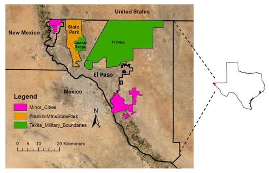
Figure 1.
The state park, military reservations, minor cities, and boundaries comprising El Paso, Texas, county utilized in this study.
El Paso County was home to more than 566 thousand people in 2000 and increased to approximately 840 thousand people in 2018. The population is estimated to increase to over 952,000 by 2030 [30,33]. The county consists of several minor cities and towns, including Horizon City, Socorro, Clint, Vinton, and Anthony. The city of El Paso (hereafter El Paso) is by far the largest populous city in the county and was ranked 22nd among the most populous cities in the nation by 2018 [30] with an estimated population of over 683 thousand. El Paso accounted for 70% of the counties’ population in 2018 [30].
Unlike many other cities that can expand in various directions around urban centers, such as Phoenix and Las Vegas, El Paso’s growth is restricted due to several jurisdiction entities. The jurisdictions include a country (Mexico) and states (New Mexico and Chihuahua, Mexico) that lie adjacent to the study area. This uniqueness adds to the complexity and interest of understanding the growth patterns of not only an urbanized area located within a desert region but the second-largest U.S.–Mexico border city next to San Diego, CA. El Paso wraps around the southern tip of the Franklin Mountains and extends along the west and east side of the mountain. On the eastern side of the Franklin Mountain, the city can expand northward and eastward. However, new development is limited on the western side as the boundaries to Mexico and New Mexico are in close proximity. The city is comprised of eight representative districts. Each district elects a representative to reside on the City Council for administering/amending the cities legislative duties, including budgets, taxes, policies, and ordinances. With the Council’s efforts, the city adopted a comprehensive plan titled “Plan El Paso” in March of 2012 to provide guidance for economic, health, and physical concerns utilizing policy and regulations for the expanding city and surrounding community [29]. Incorporating a discussion of past and current trends of the region and applying goals and policies to address community concerns, Plan El Paso provides the vision of El Paso’s future for the next 25 years. As part of urban management, the Plan provides a future land use map that indicates designated areas for preferred immediate growth and possible annexation areas outside the city limits for long-term growth. Management of these goals is implemented through city budgets, city approval for development projects that are in accordance with the Plan, economic incentives, and City Council to ensure their decisions are in agreement with the Plans’ goals.
2.2. Data Collection
The National Land Cover Database (NLCD) is a result of a collaboration among federal agencies (Multi-Resolution Land Characteristics Consortium) and was the pioneer in providing consistent land cover information for the conterminous United States utilizing Landsat imagery [13,34]. The most recent version of NLCD is the 2016 product suite, which covers a 15-year period from 2001–2016 (2001, 2004, 2006, 2008, 2011, 2013, and 2016) for the Continental United States (CONUS) using categorical land cover information. The suite was developed based on four extensive mapping techniques, which include: spectral signatures, time-dependent spectral succession and trajectory patterns, spectral patch shape, and ancillary data [35]. This comprehensive method updates previous NLCD releases and allows a comparison of land cover data among the time periods provided [34].
The NLCD 2016 provides 30-m revolution images with eight class categories for CONUS [35]. Within each class category, the categories are further divided into classification descriptions. The developed class category consists of four classification descriptions based on varying impervious surface percentages (Table 1). The developed class is updated every 5 years beginning in 2001. The remaining categories pertain to non-impervious areas, such as water, barren land, forest, and shrubland. Since the focus of this study is on urban expansion, two categories of land-use were utilized: 1) developed and 2) undeveloped (barren). The developed land-use combines the four NLCD impervious surface descriptions, while the undeveloped (barren) land-use representing the remaining classes. The NLCD 2016 classes and descriptions allow for the creation of land-use maps, which provide a visual interpretation of land-use for regions of interest.

Table 1.
National Land Cover Database (NLCD) land cover classification and classes used in this research.
The NLCD 2016 suite, which encompasses land-cover from 2001–2016, is the most accurate release in NLCD history [34] and has been used extensively to study urbanization [13,35,36]. However, an argument has been posed to question past versions of NLCD reliability in forest areas where satellite imagery does not detect minor development [36]. Shrestha et al. (2012) [13] found that the NLCD, in particular 2001 NLCD, was “very accurate” for assessing developed areas in the treeless desert region of Phoenix, due to the lack of satellite obstruction from the treeless environment. It was recommended that NLCD be used in analyzing urban dynamics in desert environments to save time and resources [13]. Due to this recommendation and its extensive use, the NLCD land cover data was adopted for this study and its corresponding data availability timeframe from 2001 to 2016.
FRAGSTATS is a popular computer software program that generates landscape metrics and was developed in 1995 by Dr. Kevin McGarigal and Barbara Marks of Oregon State University [36]. Past research study areas using FRAGSTATS include India, Canada, and China [36,37,38]. FRAGSTATS was used in this study to determine the landscape metrics for the study area.
2.3. Predicted Future Land-Use
Predicting future land-use has been used extensively in the past 15 years [3] for urban development planning and management using the CA-Markov model [7,8,39,40]. CA-Markov is a hybrid model that incorporates past spatial and temporal trends to predict future projections. CA (Cellular Automata) is limited due to its inability to consider outside factors, such as physical and socioeconomic factors [41]. Therefore, a quantitative system must be included, such as the Markov Chain model. The probability model, Markov Chain model, is used extensively in analyzing land-use change due to its stochastic process of predicting the probability of change from one state to another using the preceding state conditions [8,42,43]. The analysis is conducted for a specific time period, with the start time as the baseline and is discrete in time and state. The Markov model is based on transition probability [44]. Thus, it results in a transition probability matrix, which describes the probability of a state transitioning into another in matrix form. The following illustrates the Markov Chain probability matrix:
where
- ;
- ;
- ;
- .
Along with the Markov probability matrix, suitability maps are also implemented in the CA-Markov model. Suitability maps illustrate the probability of a cells’ transition by utilizing transition rules for each land-use class. Transition rules incorporate socio-economic and/or physical factors’ influence on land-use change through the use of multi-criteria evaluation (MCE) [43]. This study implemented two physical factors: (1) distance from developed areas and (2) distance from roadways due to the availability of data, while the constraints were the developed area and roadways themselves (Figure 2). The constraints dictate where urban expansion could not occur.
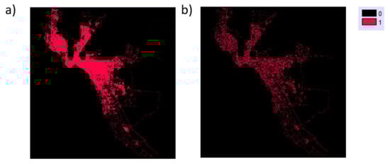
Figure 2.
Input data of constraints utilized in this study (a) developed area (b) roads. (0 = non-constraint area, 1 = constraint area).
MCE combines transition rules for constraints and factors to form a single index accurately predicting land-use change [8]. Constraints do not allow class expansion, while factors provide a probability of class expansion typically based on distance [10]. The result of the MCE analysis is presented as suitability maps. The Markov transition probability matrix, along with suitability maps, are then applied in the CA-Markov model, where spatial relations among states are analyzed. Cellular Automata (CA) considers discrete spatial and time configurations for complex arrangements. Therefore, the study time period is incorporated, along with the state of neighboring cells. The hybrid model is expressed as follows [44]:
- ;
- ;
- ;;
- .
CA is an iterative process that is composed of cells, each cell changes/maintains a state at each time iteration based on rules provided by the transition probability matrix and area and can be utilized from the simplest of patterns to complex algorithmic problems [45]. As a result, cells within close proximity to existing areas possess an increase in transition probability resulting in land-use changes [44]. The CA-Markov output provides a projected land cover map of the time period in question.
The advantage of the hybrid CA-Markov model is that the Markov Chain model considers the change of a cell from one point in time to another. However, the influence of the neighboring cells is not considered, whereas the CA model does consider the state of the surrounding cells. The state of the neighboring cells influences the potential for a cell to change the state [39]. The disadvantage of the CA-Markov model is the lack of integrating socio-economic influence within the expansion scenario. However, integration of models, such as fuzzy logic, logistic regression, and multiple criteria evaluation, allows the inclusion of socio-economic factors, such as population and income. These methods incorporate weighted factors from historical data, policies, surveys, and literature review [44].
Once the results are provided, a verification of the CA-Markov model output is conducted utilizing an error matrix and Kappa coefficient. An error matrix includes various probability terms that describe the performance of the classification data [27,46], whereas the Kappa coefficient provides an understanding of the classified data compared to the classification by chance. The CA-Markov model is used to predict the land-use of a time period with reference data. The predicted results are compared to the reference data for validation using the accuracy assessment procedure. If the accuracy assessment is acceptable, the projection of future land-use is predicted [7,8,39].
2.4. Past and Predicted Landscape Metrics
Using the projected and NLCD land-use data, FRAGSTATS, an extensively adopted program to calculate landscape metrics for urban spatiotemporal dynamics [11,13,47,48], was utilized in determining the landscape metrics for El Paso’s urban growth areas for this study. A minimal amount of landscape metrics can demonstrate the urban dynamic behavior within a study area [11]. Six metrics were utilized for the developed class level as this class is the focus of this study (Table 2). The metrics focus on the developed land-use type, as this class is the focus of this study. The metrics include the percentage of developed landscape (PLAND), number of patches (NP), mean patch area (AREA_MN), edge density (ED), landscape shape index (LSI), and patch density (PD). The term patch is used extensively in landscape metrics and refers to the cluster of joining cells with the same land-use type [49]. Patches provide an understanding of possible fragmentation within the class type. Edge density and landscape shape index provides a perspective of shape irregularity of the class type.
Table 2.
Class metrics and descriptions utilized in this study for urban dynamic analysis.
2.5. Panel Data Analysis
In order to examine the relationship between landscape metrics and their possible impacts on electricity consumption, a panel data analysis was adopted. Electricity consumption data for the area was graciously provided by the electricity company which services the study area (El Paso Electric Company). The data consisted of yearly average electricity usage (kWh) by the district. Incorporating the results from the past and future landscape results and the obtained electricity consumption data, a panel data analysis was conducted. Panel data analysis consists of three models: pooled regression, variable intercepts, and constant coefficients, and variable intercepts and variable coefficients models. Pooled regression considers constant coefficients and is expressed as the following [17,50]:
where:
- ;
- ;
- ;
- ;
- ;
- ;.
The variable intercepts and constant coefficients model pertain to both the fixed and random-effects models. Fixed-effects model applies to non-random sampling/selection panel data [51] and assumes “the intercept αi, is uncorrelated with xit and a constant value for i” [17,52], whereas the random-effects model applies to random sampling/selection data [51] where “αi is affected by xit, and αi involves not only a constant but also a random term caused by xit” [17,52]. The fixed/random-effects model is expressed as:
where:
- ;
- ;
- ;
- ;
- ;
- ;
- .
The third model indicates coefficients may vary among individuals, as demonstrated by the term as follows:
where:
- ;
- ;
- ;
- ;
- ;
- ;
- .
An F-test is first conducted to verify which model to incorporate. The hypothesis states:
where H1 refers to the pooled regression model, where intercepts and coefficients are constant for individuals and time. H2 states intercepts are variable and coefficients are constant. If H1 is accepted, then the pooled regression model is incorporated. If H2 is accepted, intercepts are variable and coefficients are constant [52,53]. The Hausman test is then implemented to indicate whether the fixed or random model is implemented.
The panel data analysis is limited to the number of time-series observations, and t is at least as large as the total number of independent variables, indicating that t ≥ k +1. For this study, the number of time periods, t = 2, and the number of independent variables, k = 6. Therefore, a single independent variable at a time must be analyzed for this study.
3. Results and Discussions
3.1. Land-Use Change Analysis
The land-use change analysis for this study incorporated land-use maps and the corresponding database management techniques to analyze land-use change over time. The land-use maps were generated based on the developed category, which combines all sub-categories within the NLCD developed category vs barren (undeveloped) class. The goal was to provide a comprehensive and detailed understanding of urban development within the region. The land-use classification process resulted in four land-use maps, which provided a detailed understanding of where the concentration of urban expansion took place within El Paso County from 2001 to 2016, excluding the military reservation areas and Franklin Mountains State Park.
At the county level, the results demonstrated the developed class increased by 24% from 2001–2016, with 68% of the expansion occurring within the City of El Paso. Figure 3 illustrates the specific areas of the counties’ urban growth from 2001–2016, with expansion concentrated within the city of El Paso.
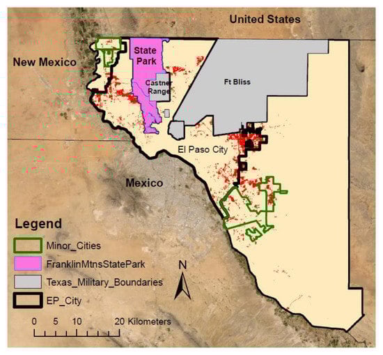
Figure 3.
Urban growth from 2001 to 2016 within the County of El Paso, with a concentration of growth occurring with El Paso city.
The county saw the largest development growth occur from 2001 to 2006 at 12.73%, and continued to decrease from 5.66% (2006–2011) to 4.15% (2011–2016). Similarly, the city of El Paso (herein El Paso) grew by over 21% from 2001 to 2016 and experienced the largest developmental growth from 2001–2006 at almost 12% and continued to decline to 5% (2006–2011) and 3.25% (2011–2016). The growth percentages and patterns of El Paso reciprocated the growth patterns at the county level.
Due to the majority of development occurring within the city limits of El Paso, the 8 districts comprising the city were further analyzed to determine the amount and location of growth within the city boundary. Each districts’ urban growth was determined relative to the total growth within the city to allowed a comparison between the districts. From 2001–2016, the districts with the highest city contribution of growth were Districts 5 and 1 at approximately 31.5% and 28.00%, respectively. Districts 6 and 4 followed at 14.84% and 12.25%, respectively. The remaining districts contributed less than 6% of the cities’ urban growth as demonstrated in Figure 4.
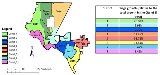
Figure 4.
Results of district percentage of urban growth relative to city growth from 2001 to 2016.
District 6 is the third-highest contributor to growth at 14.84% from 2001–2016. However, District 6 growth mainly occurred from 2001–2006. After 2006, District 6 seen a drastic decline in its growth at 7.54% (2006–2011) and 6.32% (2011–2016). Districts 5, 1, and 4 had the largest contribution of growth and ranked in top contributing districts throughout 2001–2016. The contribution is illustrated among the 2006–2011 and 2011–2016 time series. For 2001–2006, District 1 and 5 were the top 2 districts in growth, followed by Districts 6 and 4. Due to Districts 5, 1, and 4 consistent top growth relative to the city, these districts were further analyzed for urban dynamic patterns
3.2. Landscape Metrics
To quantify the urban dynamics that transpired within the three city districts (Districts 5, 1, and 4) exhibiting the majority of urban growth, class-level metrics were utilized due to the limited number of classes (developed and undeveloped). Six metrics were selected for the developed class-level metrics (PLAND, NP, AREA_MN, ED, LSI, PD), as previously discussed, which were deemed acceptable to provide an understanding of the landscape [11,13,17]
The results for the class-level metrics were relative to the district itself. The developed percentage of landscape increased linearly for District 5 from 27% in 2001 to 74% in 2016 (Figure 5). Districts 1 and 4 also exhibited an increase in development from 36% to 51.5% and 27% to 33%, respectively. This reflects the vast urban growth within District 5 and the consistent growth that transpired within Districts 1 and 4 for the 15-year study period.
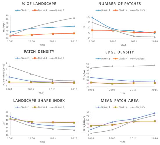
Figure 5.
Class metrics results for the developed class within Districts 1, 4, and 5 from 2001 to 2016.
Urban growth can occur with fragmented patterns of patches. Patches are clusters of cells with the same land-use type. The number of patches significantly decreased for Districts 5 and 1. District 5 decreased by 73% of the number of patches from 2001 to 2016. District 1 had an approximate 63% decrease in the number of patches. District 4 had a smaller decrease in the number of patches at over 16.5%. This indicates that District 5 and 1 had an extensive decrease in fragmentation of the developed land-use. This also illustrates in-fill development to connect the patches of existing urban development. Thus, the significant decrease in patch density for District 5, a relative decrease in District 1, and a slight decrease in District 4. The edge density for District 5 decreased, while remained relatively constant for the remaining districts. This can be attributed to Districts 5 drastic urban growth that encompasses a large amount of the landscape, while the remaining districts saw relatively constant edge density due to the smaller developed area relative to the districts themselves. In other words, the landscape of the districts is not dominated by the developed area. Therefore, the length of all edge segments per hectare remained relatively constant. As the developed class increased, the mean patch area also significantly increased for Districts 5 and 1. As the number of patches decreased, the complexity of the shape of the developed class also decreased as illustrated with the landscape shape index (LSI). The decrease in LSI indicates a decrease in the irregularity of the developed class shape.
The percentage of developed landscape demonstrates that District 5 experienced a linear growth rate from 2001–2016, compared to the remaining districts (Districts 1 and 4) which experienced gradual continued growth. As the districts expanded, fragmentation decreased as illustrated by the decrease in the number of patches and patch density, as well as the increase in mean patch area. The increase in urban development also decreased the irregularity of the developed shape areas within the districts.
3.3. Future Projection Land-Use Change Analysis
To model future urban expansion, the model itself was first verified using existing data. Verification of the CA-Markov model was conducted using the acquired NLCD data for 2001 and 2011 to predict the land-use for 2016. Adopting the Anderson classification system, all of the accuracy terms exceeded the stringent 85 percent minimum accuracy [54] for both the county and city level as illustrated in Table 3. The Kappa coefficient rated “almost perfect”, above 81% accuracy, for both levels. This is consistent with previous research where the CA-Model accuracy was found to possess a Kappa coefficient of 81% and greater [7,8,42,44], and an overall accuracy of 91% [44]. The assessment results verify the use of the CA-Markov method for predicting future land-use in the El Paso area.
Table 3.
Cellular Automata (CA)-Markov accuracy results utilizing land cover data for 2001 and 2011 to predict the 2016 land cover for the El Paso region.
Once the model was verified, the resulting 2031 land-use map prediction was determined. Using the predicted map, a change analysis was conducted. Comparing the 15-year incremental time periods (2001–2016 and 2016–2031), the county urban growth from 2016 to 2031 decreased to 18.24%, in comparison to the previous 15-year period (2001–2016) which possessed a 24% change in development (Table 4). The decline is expected, as previously discussed, the 5-year incremental time periods from 2001–2016, continuously declined, as well.
Table 4.
El Paso County land-use and change percentage for 15-year increments between 2001 and 2031.
Of the projected expansion that occurred within the county, 51% occurred within the city of El Paso compared to approximately 66% for 2001–2016. Therefore, urban growth is projected to be evenly split within the city limits of El Paso and outside the city boundary. Due to the equally projected contribution of growth, both areas’ expansion patterns were analyzed. The 8 districts within the city were analyzed to determine the locations of concentrated growth within the cities’ boundary. District 1 is projected to have the largest percentage of growth at roughly 24% (Figure 6). Followed by Districts 4 and 5 at 22.66% and 13.76%, respectively. Districts 8 and 2 followed with projected percentage growth at 11.91% and 11.43%, respectively. The remaining districts possess less than 9% growth. Comparing the districts’ 15-year growth percentages between 2001–2016 and 2016–2031, Districts 4, 8, and 2 possess the largest increase in growth percentage. District 4 projects the highest increase at 10.41% compared to 2001–2016. Districts 8 and 2 have an increase of 8.42% and 5.5%. District 4 contained the cities’ majority of barren land for development in 2016 at 41.20%. Therefore, it is logical that District 4 would have an increase in development. District 1 contained the largest amount of the cities barren land in 2016 at 27.27%. However, the projection indicates that District 1 has a decrease in growth percentage by 3.61% compared to 2001–2016. District 5 exhibits the largest difference in growth percentage among the 15-year comparisons, at nearly 18%. The substantial growth that District 5 possessed during 2001–2016 may have an impact on the projected growth.
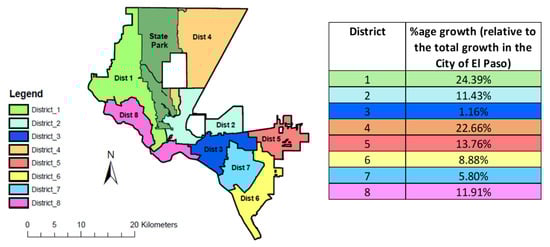
Figure 6.
Results of district percentage of urban growth relative to city growth from 2016 to 2031.
Outside the city limits of El Paso, 49% of the projected growth for 2031 is expected to occur. The county of El Paso is comprised of several cities including El Paso, Anthony, Clint, Horizon City, Socorro, Vinton, and Fabens. With the exception of El Paso, the cities’ total contribution to the counties’ projected growth in 2031 is approximately 25%. The majority of future growth is to occur outside the limits of the surrounding cities. The projected growth is concentrated in 3 main areas: Area 1) adjacent to District 5, Area 2) adjacent to District 6, and Area 3) adjacent to District 1 along the New Mexico border (Figure 7). Area 1 and 2 are located within the potential annexation areas proposed by the city’s comprehensive plan, Plan El Paso [29]. The potential annexation spaces will be utilized for urban growth by 2031. Area 3 is not located within a preferred annexation area. Therefore, the growth in Area 3 should be mitigated through policies to encourage growth within the designated immediate growth or possible annexation areas.
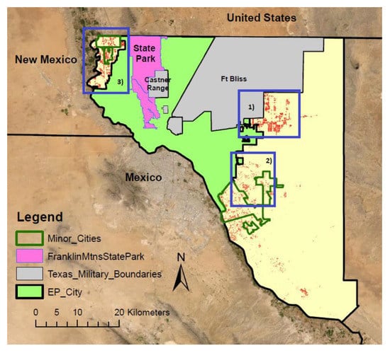
Figure 7.
Projected 2031 urban growth clusters outside the city limits of El Paso.
3.4. Future Projection Landscape Metrics
Landscape metrics were analyzed for Districts 1, 4, and 5 to provide an understanding of the projected growth patterns for 2031. The percentage of the developed area (PLAND) for District 1 increased by 18% (Figure 8). The number of patches (NP) decreased by 24%, indicating infill within the existing developed area. The patch density (PD), measuring the number of patches per 100 hectares of developed area, decreased slightly (23%) compared to 2016; also indicates infill development. Edge density (ED), which measures the total edge distance per developed patch, and the landscape shape index (LSI), indicates shape regularity, decreased. This suggests that, as the developed class increased, the edge length of the developed patches decreased, and the irregularity of the developed class decreased. The mean patch area (AREA_MN) also increased, due to the increase in the developed class.
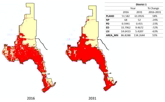
Figure 8.
Comparison of District 1 developed class (red) in 2016 (left) and 2031 (right) and class metrics results for 2016 and 2031.
District 5 possesses similar results as District 1 (Figure 9). The percentage of the developed area (PLAND) increased by 19%. The number of patches (NP), patch density (PD), and edge density (ED) decreased indicating infill within District 5. The mean patch area increase of 77% is indicative of the growth in the developed class area.
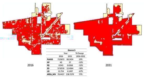
Figure 9.
Comparison of District 5 developed class (red) in 2016 (left) and 2031 (right) and class metrics results for 2016 and 2031.
District 4 possesses slightly different metric results compared to Districts 1 and 5. The percentage of the developed area (PLAND) also increased in District 4 by 24% (Figure 10). The number of patches (NP) and patch density (PD) show a slight increase at 27% for both metrics, suggesting possible fragmentation within District 4. The decrease in edge density (ED) suggests the patch areas increased. The decrease in landscape shape index (LSI) indicates a decrease in shape irregularity for the developed class. The mean patch area relatively stayed constant, suggesting the developed growth area relative to the number of patches remained constant. According to the landscape metrics, Districts 1 and 5 experience infill development. However, District 4 experiences slight fragmentation compared to the other districts. The rate of infill for District 4 is slower than the other districts. Therefore, infill should be encouraged for District 4.
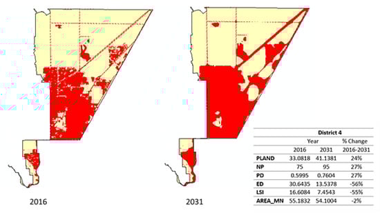
Figure 10.
Comparison of District 4 developed class (red) in 2016 (left) and 2031 (right) and class metrics results for 2016 and 2031.
3.5. Urban Form and Electricity Consumption
The panel data analysis was implemented to investigate the relationship between urban form and electricity consumption using STATA software. To determine which panel regression model to use, the f-test was conducted. The constant intercepts and coefficients model contained one metric that was significant (Table 5), which was the mean patch area (AREA_MN), whereas the variable intercepts and constant coefficients indicate three metrics were significant, including the percentage of landscape (PLAND), landscape shape index (LSI), and mean patch area (AREA_MN). R-squared (R2) was also considered when choosing a model, due to its ability to interpret how well the model fits the data. The variable intercepts and constant coefficients model possess significantly higher R2 values than the constant intercepts and coefficients model, indicating this model fits the data well. Therefore, the variable intercepts and constant coefficients model was further analyzed.
Table 5.
F-test results among class metrics to determine which panel regression to use in analysis for this study.
The Hausman test was implemented to determine if fixed or random effects should be implemented in the variable intercepts and constant coefficients model, using the following hypothesis:
Ho = random-effects model selected (null hypothesis);
H1 = Ho is not true, fixed effect model selected.
Using a significance level, α, of 0.10, the Hausman test results indicate the null hypothesis cannot be rejected (Table 6). Therefore, the random-effects model was selected for analysis.
Table 6.
Hausman test results among class metrics to determine if a fixed or random-effects model should be implemented for this study.
The panel data analysis utilizing random-effects was performed to understand the impact of a metric on electricity consumption. The random-effects model indicates that one metric is significantly correlated with electricity consumption, mean patch area (AREA_MN), with a 0.01 significant level (Table 7). The remaining metrics were not significantly correlated with electricity consumption for this study.
Table 7.
Random effects panel data analysis results for class metrics.
The mean patch area describes the sum of all developed patch areas divided by the number of patches for a class. This metric increased within each district throughout the study period, with the exception of District 4, indicating that as the developed area increased, fragmentation decreased (Table 8). Districts 1 and 5 projected a decrease in the number of patches (NP) and an increase in the percentage of developed area; thus, an increase in mean patch area. However, District 4 projected a relatively constant mean patch area from 2016 to 2031. This is due to the increase in the developed area (24%) and the number of developed patches (27%) increasing from 2016 to 2031.
Table 8.
Districts 1, 4, and 5, class metrics percentage change from 2016 to 2031.
Electricity consumption will increase by 4.1058 (106 kWh) for every unit increase in the mean patch area. This indicates that District 1 will increase by 209.27 (106 kWh), exhibiting a linear increase in electricity consumption (Figure 11). District 5 increase of 262.035 (106 kWh), indicating a sharp increase within the 5-year period from 2011 to 2016. However, a slight decline in electricity consumption from 2016 to 2031. This is indicative of the decline in urban development within the district. District 4 increases the least at 18.96 (106 kWh). This is due to District 4 experiencing a relatively constant mean patch area, AREA_MN, from 55.1832 (2016) to 54.1004 (2031).
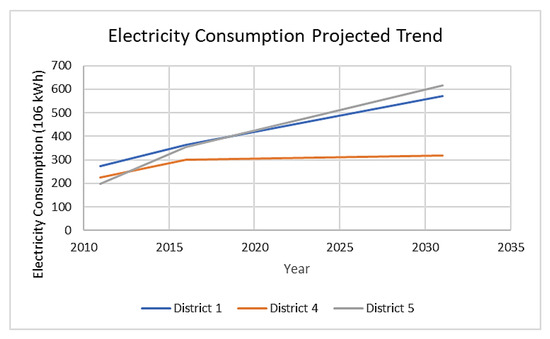
Figure 11.
Projected electricity consumption trend utilizing 2011, 2016, and projected 2031 data from this study.
District 1 and 5 findings are consistent with recent research, as urban areas expand consequentially electricity consumption increases [17,47]. However, additional factors of fragmentation, such as the number of patches (NP) and the percentage of developed area, were found to be correlated with energy consumption [47]. This study did not support this finding. It is suggested to increase the number of time periods analyzed and the number of metrics in order to provide a better understanding of the relation of landscape metrics and electricity consumption over time.
4. Conclusions
This study provides a deeper understanding of urban development trends within the past 15-years (2001–2016) and projected urban growth for the next 15-years (2031) of the El Paso region by analyzing concentrated locations of development. Previous research on studying urban trends solely for the El Paso area is limited. It was concluded that El Paso County and El Paso city exhibited similar growth trends. The urban expansion was highest within the 2001–2006 5-year period. The vast majority of the counties’ growth transpired within the city of El Paso for both the 15-year and 5-year incremental study period. Within the city, the consistent growth occurring within District 5 (east side), 1 (west side), and 4 (northeast), with District 5 experiencing the largest growth rate. District 6 experienced extensive growth between 2001 to 2006 but drastically decreased after this time period. Due to consistent and high growth rates within District 5, 1, and 4, these districts’ landscape patterns were further analyzed. The predicted county urban growth is expected to decrease to 18.24% from 2016 to 2031, compared to the 24% urban growth from 2001 to 2016. The 15-year projected development growth is expected to be evenly distributed between the city of El Paso and outside the city limits at 51% and 49%, respectively. The leading districts in projected growth are similar to the previous 15 years with Districts 1, 4, and 5 experienced the concentration of growth. However, the order is predicted to change with District 1 expected to experience the highest growth, followed by District 4 and 5. Districts 1 and 4 coincide with Plan El Paso’s Comprehensive Plan proposed policies, which indicate District 1 and 4 are preferred districts for immediate growth. District 4 experienced projected growth within the districts’ designated area for immediate growth. However, District 1 predicts growth outside of the district’s designated area for immediate growth. This may suggest possible fragmentation of future development. District 5 expansion is expected, as the district continues to expand within the city’s plan for the designated suburban area for this district. Outside the city limits of El Paso, urban growth adjacent to Districts 5 and 6 occur within potential annexation areas in accordance with the city’s comprehensive plan, Plan El Paso. The growth projected adjacent to District 1 (Area 3) does not occur within a potential annexation area. Therefore, actions should be taken to mitigate growth within this area and encourage growth within the designated immediate or possible annexation areas. The landscape metrics indicate the percentage of developed landscape within District 5 experienced linear growth from 2001–2016, compared to the remaining districts (Districts 1 and 4) which experienced gradual continual growth. As the districts expanded, fragmentation decreased as illustrated by the decrease in the number of patches and patch density, and the increase in mean patch area. The increase in urban development also decreased the irregularity of the developed shape areas within the districts. Thus, indicating possible infill with Districts 1 and 5. However, District 4 experienced slight fragmentation compared to the other districts. The rate of infill for District 4 is slower than the other districts, suggesting infill should be encouraged for District 4. The projected growth patterns are suggested to be managed utilizing the implementation tools discussed in Plan El Paso, including development approvals that are strictly in accordance with the comprehensive plan [29]. District 1 and 5 findings are consistent with recent research; as urban areas expand, consequentially, electricity consumption increases [53,55]. However, additional factors of fragmentation, such as the number of patches (NP) and the percentage of developed area, were found to be correlated with energy consumption [55] in past research. This study did not support this finding. Therefore, continued research will be conducted to expand the study time period and incorporate additional metrics to provide a better understanding of the relation of landscape metrics and electricity consumption over time.
Author Contributions
Conceptualization, J.M.M. and A.A.R.; methodology, J.M.M. and A.A.R.; software, J.M.M.; validation, J.M.M.; formal analysis, J.M.M.; data curation, J.M.M., A.A.R.; writing—original draft preparation, J.M.M.; writing—review and editing, A.A.R.; visualization, J.M.M.; supervision, A.A.R. All authors have read and agreed to the published version of the manuscript.
Funding
This research received no external funding.
Conflicts of Interest
The authors declare no conflict of interest.
References
- United Nations World Population Projected to Reach 9.8 billion in 2050, and 11.2 billion in 2100. Available online: https://www.un.org/development/desa/en/news/population/world-population-prospects-2017.html (accessed on 31 January 2020).
- United Nations Sustainable Cities and Human Settlements: Sustainable Development Knowledge Platform. Available online: https://sustainabledevelopment.un.org/topics/sustainablecities (accessed on 19 December 2019).
- Bureau, U.C. Population Trends in Incorporated Places: 2000 to 2013. Available online: https://www.census.gov/library/publications/2015/demo/p25-1142.html (accessed on 8 January 2020).
- United Nations. World Urbanization Prospects: The 2018 Revision; United Nations: New York, NY, USA, 2018; ISBN 978-92-1-148319-2. [Google Scholar]
- Tv, R.; Aithal, B.H.; Sanna, D.D. Insights to urban dynamics through landscape spatial pattern analysis. Int. J. Appl. Earth Obs. Geoinf. 2012, 18, 329–343. [Google Scholar] [CrossRef]
- Cumming, S.; Vernier, P. Statistical models of landscape pattern metrics, with applications to regional scale dynamic forest simulations. Landsc. Ecol. 2002, 5, 433–444. [Google Scholar] [CrossRef]
- Rimal, B.; Zhang, L.; Keshtkar, H.; Wang, N.; Lin, Y. Monitoring and Modeling of Spatiotemporal Urban Expansion and Land-Use/Land-Cover Change Using Integrated Markov Chain Cellular Automata Model. ISPRS Int. J. Geo Inf. 2017, 6, 288. [Google Scholar] [CrossRef]
- Chen, L.; Sun, Y.; Saeed, S. Monitoring and predicting land use and land cover changes using remote sensing and GIS techniques-A case study of a hilly area, Jiangle, China. PLoS ONE 2018, 13. [Google Scholar] [CrossRef]
- Sudhira, H.S.; Ramachandra, T.V.; Jagadish, K.S. Urban sprawl: Metrics, dynamics and modelling using GIS. Int. J. Appl. Earth Obs. Geoinf. 2004, 5, 29–39. [Google Scholar] [CrossRef]
- Aburas, M.M.; Abdullah, S.H.; Ramli, M.F.; Ash’aari, Z.H. Measuring and Mapping Urban Growth Patterns Using Remote Sensing and GIS Techniques. Peranika J. Sch. Res. Rev. 2017, 3, 55–69. [Google Scholar]
- Wu, J.; Jenerette, G.D.; Buyantuyev, A.; Redman, C.L. Quantifying spatiotemporal patterns of urbanization: The case of the two fastest growing metropolitan regions in the United States. Ecol. Complex. 2011, 8, 1–8. [Google Scholar] [CrossRef]
- Flores, E.S. Land cover change and landscape dynamics in the urbanizing area of a Mexican border city. In Proceedings of the ASPRS 2008 Annual Conference, Oregon, Portland, 28 April–2 May 2008. [Google Scholar]
- Shrestha, M.K.; York, A.M.; Boone, C.G.; Zhang, S. Land fragmentation due to rapid urbanization in the Phoenix Metropolitan Area: Analyzing the spatiotemporal patterns and drivers. Appl. Geogr. 2012, 32, 522–531. [Google Scholar] [CrossRef]
- United Nations, Modernizing Energy Systems Can Reduce Primary Energy Consumption in Heating and Cooling by up to 50%—UN Report, United Nations Sustainable Development. Available online: https://www.un.org/sustainabledevelopment/blog/2015/02/modernizing-energy-systems-can-reduce-primary-energy-consumption-in-heating-and-cooling-by-up-to-50-un-report/ (accessed on 9 June 2020).
- US Energy Information Administration Frequently Asked Questions (FAQs)—U.S. Energy Information Administration (EIA). Available online: https://www.eia.gov/tools/faqs/faq.php (accessed on 8 June 2020).
- Abbasabadi, N.; Ashayeri, M.; Azari, R.; Stephens, B.; Heidarinejad, M. An integrated data-driven framework for urban energy use modeling (UEUM). Appl. Energy 2019, 253, 113550. [Google Scholar] [CrossRef]
- Zhao, J.; Thinh, N.X.; Li, C. Investigation of the Impacts of Urban Land Use Patterns on Energy Consumption in China: A Case Study of 20 Provincial Capital Cities. Sustainability 2017, 9, 1383. [Google Scholar] [CrossRef]
- Li, C.; Song, Y.; Kaza, N. Urban form and household electricity consumption: A multilevel study. Energy Build. 2018, 158, 181–193. [Google Scholar] [CrossRef]
- Sexton, J.O.; Song, X.-P.; Huang, C.; Channan, S.; Baker, M.E.; Townshend, J.R. Urban growth of the Washington, D.C.–Baltimore, MD metropolitan region from 1984 to 2010 by annual, Landsat-based estimates of impervious cover. Remote Sens. Environ. 2013, 129, 42–53. [Google Scholar] [CrossRef]
- Yuan, F.; Sawaya, K.E.; Loeffelholz, B.C.; Bauer, M.E. Land cover classification and change analysis of the Twin Cities (Minnesota) Metropolitan Area by multitemporal Landsat remote sensing. Remote Sens. Environ. 2005, 98, 317–328. [Google Scholar] [CrossRef]
- DiBari, J.N. Evaluation of five landscape-level metrics for measuring the effects of urbanization on landscape structure: The case of Tucson, Arizona, USA. Landsc. Urban Plan. 2007, 79, 308–313. [Google Scholar] [CrossRef]
- Barud-Zubillaga, A. Urban Development under Extreme Hydrologic and Weather Conditions for El Paso-Juárez: Recommendations Resulting from Hydrologic Modeling, GIS, and Remote Sensing Analyses. Ph.D. Thesis, the University of Texas, El Paso, TX, USA, 2011. [Google Scholar]
- Neelam, T.J. Assessing the Hydrologic Impacts of Extreme Rainfall and Land Use Change on a Semiarid Watershed. M.S. Thesis, the University of Texas, El Paso, TX, USA, 2018. [Google Scholar]
- Mahmud, S. The Use of Remote Sensing Technologies and Models to Study Pollutants in the Paso del Norte region. M.S. Thesis, the University of Texas, El Paso, TX, USA, 2016. [Google Scholar]
- Amaya, M.; Mohamed, M.; Pingitore, N.; Aldouri, R.; Benedict, B. Community Exposure to Nighttime Heat in a Desert Urban Setting, El Paso, Texas; Social Science Research Network: Rochester, NY, USA, 2016. [Google Scholar]
- Miyazono, S.; Patiño, R.; Taylor, C.M. Desertification, salinization, and biotic homogenization in a dryland river ecosystem. Sci. Total Environ. 2015, 511, 444–453. [Google Scholar] [CrossRef] [PubMed]
- Mubako, S.; Belhaj, O.; Heyman, J.; Hargrove, W.; Reyes, C. Monitoring of Land Use/Land-Cover Changes in the Arid Transboundary Middle Rio Grande Basin Using Remote Sensing. Remote Sens. 2018, 10, 2005. [Google Scholar] [CrossRef]
- Everett, A.L. Impacts of Environmental Changes to the Middle Rio Grande Landscape on Ysleta Del Sur Pueblo’s Cultural and Ceremonial Sustainability. M.S. Thesis, the University of Texas, El Paso, TX, USA, 2016. [Google Scholar]
- City of El Paso Plan El Paso, El Paso, TX, USA. 2012. Available online: https://www.elpasotexas.gov/planning-and-inspections/plan-el-paso (accessed on 25 June 2020).
- U.S. Census Bureau. U.S. Census Bureau QuickFacts: El Paso County, Texas; United States. Available online: https://www.census.gov/quickfacts/fact/table/elpasocountytexas,US (accessed on 8 January 2020).
- United States Department of Agriculture Census of Agriculture—2017 Census Publications-State and County Profiles—Texas. Available online: https://www.nass.usda.gov/Publications/AgCensus/2017/Online_Resources/County_Profiles/Texas/index.php (accessed on 5 January 2020).
- U.S. Army Bases—History, Locations, Maps and Photos 2018. Available online: http://armybases.org/fort-bliss-tx-texas/ (accessed on 3 January 2020).
- Texas Department of State Health Services Population Data (Projections) for Texas Counties. 2020. Available online: https://www.dshs.texas.gov/chs/popdat/st2020.shtm (accessed on 8 January 2020).
- Wickham, J.; Homer, C.; Vogelmann, J.; McKerrow, A.; Mueller, R.; Herold, N.; Coulston, J. The Multi-Resolution Land Characteristics (MRLC) Consortium—20 Years of Development and Integration of USA National Land Cover Data. Remote Sens. 2014, 6, 7424–7441. [Google Scholar] [CrossRef]
- Homer, C.; Dewitz, J.; Jin, S.; Xian, G.; Costello, C.; Danielson, P.; Gass, L.; Funk, M.; Wickham, J.; Stehman, S.; et al. Conterminous United States land cover change patterns 2001–2016 from the 2016 National Land Cover Database. ISPRS J. Photogramm. Remote Sens. 2020, 162, 184–199. [Google Scholar] [CrossRef]
- MRLC National Land Cover Database 2016 (NLCD2016) Legend|Multi-Resolution Land Characteristics (MRLC) Consortium. Available online: https://www.mrlc.gov/data/legends/national-land-cover-database-2016-nlcd2016-legend (accessed on 31 January 2020).
- Bounoua, L.; Nigro, J.; Zhang, P.; Thome, K.; Lachir, A. Mapping urbanization in the United States from 2001 to 2011. Appl. Geogr. 2018, 90, 123–133. [Google Scholar] [CrossRef]
- Kew, B.; Lee, B.D. Measuring Sprawl across the Urban Rural Continuum Using an Amalgamated Sprawl Index. Sustainability 2013, 5, 1806–1828. [Google Scholar] [CrossRef]
- Jokar Arsanjani, J.; Helbich, M.; Kainz, W.; Darvishi Boloorani, A. Integration of logistic regression, Markov chain and cellular automata models to simulate urban expansion. Int. J. Appl. Earth Obs. Geoinf. 2013, 21, 265–275. [Google Scholar] [CrossRef]
- Tang, J.; Di, L. Past and Future Trajectories of Farmland Loss Due to Rapid Urbanization Using Landsat Imagery and the Markov-CA Model: A Case Study of Delhi, India. Remote Sens. 2019, 11, 180. [Google Scholar] [CrossRef]
- Aburas, M.M.; Ho, Y.M.; Ramli, M.F.; Ash’aari, Z.H. The simulation and prediction of spatio-temporal urban growth trends using cellular automata models: A review. Int. J. Appl. Earth Obs. Geoinf. 2016, 52, 380–389. [Google Scholar] [CrossRef]
- Subedi, P.; Subedi, K.; Thapa, B. Application of a Hybrid Cellular Automaton—Markov (CA-Markov) Model in Land-Use Change Prediction: A Case Study of Saddle Creek Drainage Basin, Florida. Appl. Ecol. Environ. Sci. 2013, 1, 126–132. [Google Scholar] [CrossRef]
- Taha, H.A. Operations Research: An Introduction, 8th ed.; Pearson/Prentice Hall: Upper Saddle River, NJ, USA, 2007; ISBN 978-0-13-188923-1. [Google Scholar]
- Fu, X.; Wang, X.; Yang, Y.J. Deriving suitability factors for CA-Markov land use simulation model based on local historical data. J. Environ. Manag. 2018, 206, 10–19. [Google Scholar] [CrossRef]
- Berto, F.; Tagliabue, J. Cellular Automata (Stanford Encyclopedia of Philosophy). Available online: https://plato.stanford.edu/entries/cellular-automata/ (accessed on 12 May 2020).
- Keranen, K.; Kolvoord, R. Making Spatial Decisions Using GIS and Remote Sensing: A Workbook; Esri Press Academic: New York, NY, USA, 2014. [Google Scholar]
- Kim, J.-H.; Li, W.; Newman, G.; Kil, S.-H.; Park, S.Y. The influence of urban landscape spatial patterns on single-family housing prices. Environ. Plan. B Urban Anal. City Sci. 2018, 45, 26–43. [Google Scholar] [CrossRef]
- Megahed, Y.; Cabral, P.; Silva, J.; Caetano, M. Land Cover Mapping Analysis and Urban Growth Modelling Using Remote Sensing Techniques in Greater Cairo Region—Egypt. ISPRS Int. J. Geo Inf. 2015, 4, 1750–1769. [Google Scholar] [CrossRef]
- Turner, M.G.; Gardner, R.H. Landscape Metrics. In Landscape Ecology in Theory and Practice: Pattern and Process; Turner, M.G., Gardner, R.H., Eds.; Springer: New York, NY, USA, 2015; pp. 97–142. ISBN 978-1-4939-2794-4. [Google Scholar]
- Brooks, C. Introductory Econometrics for Finance; Cambridge University Press: Cambridge, UK, 2019; ISBN 978-1-108-52640-1. [Google Scholar]
- Seddighi, H.R. Introductory Econometrics: A Practical Approach. 2012. Available online: https://rune.une.edu.au/web/handle/1959.11/22706 (accessed on 8 July 2020).
- Hsaiao, C. Analysis of Panel Data, 2nd ed.; Cambridge University Press: Cambridge, UK, 2003. [Google Scholar]
- Chen, Y.; Li, X.; Zheng, Y.; Guan, Y.; Liu, X. Estimating the relationship between urban forms and energy consumption: A case study in the Pearl River Delta, 2005–2008. Landsc. Urban Plan. 2011, 102, 33–42. [Google Scholar] [CrossRef]
- Anderson, J.R.; Hardy, E.E.; Roach, J.T.; Witmer, R.E. A Land Use and Land Cover Classification System for Use with Remote Sensor Data; United States Department of the Interior: Washington, DC, USA, 1976.
- Wilson, B. Urban form and residential electricity consumption: Evidence from Illinois, USA. Landsc. Urban Plan. 2013, 115, 62–71. [Google Scholar] [CrossRef]
Publisher’s Note: MDPI stays neutral with regard to jurisdictional claims in published maps and institutional affiliations. |
© 2020 by the authors. Licensee MDPI, Basel, Switzerland. This article is an open access article distributed under the terms and conditions of the Creative Commons Attribution (CC BY) license (http://creativecommons.org/licenses/by/4.0/).