Article

An Improved Hybrid Highway Traffic Flow Prediction Model Based on Machine Learning

Transportation College, Jilin University, Changchun 130022, China
*
Author to whom correspondence should be addressed.
Sustainability 2020, 12(20), 8298; https://doi.org/10.3390/su12208298
Submission received: 6 September 2020 / Revised: 23 September 2020 / Accepted: 28 September 2020 / Published: 9 October 2020
(This article belongs to the Special Issue Innovative Mobility Solutions for Sustainable Transportation)

Abstract

:
For intelligent transportation systems (ITSs), reliable and accurate real-time traffic flow prediction is an important step and a necessary prerequisite for alleviating traffic congestion and improving highway operation efficiency. In this paper, we propose an improved hybrid predicting model including two steps: decomposition and prediction to predict highway traffic flow. First, we adopted the complete ensemble empirical mode decomposition with adaptive noise (CEEMDAN) method to adaptively decompose the original nonlinear, nonstationary, and complex highway traffic flow data. Then, we used the improved weighted permutation entropy (IWPE) to obtain new reconstructed components. In the prediction step, we used the gray wolf optimizer (GWO) algorithm to optimize the least-squares support vector machine (LSSVM) prediction model established for each reconstruction component and integrate the prediction results of each subsequence to obtain the final prediction result. We experimentally validated the effectiveness of the proposed approach. The research results reveal that the proposed model is useful for predicting traffic flow and its changing trends and also allowing transportation officials to make more effective traffic decisions.

1. Introduction

Reliable and accurate real-time traffic flow prediction is crucial for intelligent transportation systems (ITSs). It is a necessary prerequisite for alleviating traffic congestion, realizing traffic management, traffic control, traffic guidance, and improving road operation efficiency. Traffic flow prediction is the basis of inducing effective traffic management and alleviating traffic congestion [1,2]. The characteristics of traffic flow are periodic, randomness, temporal, and spatial correlations. Accurately predicting traffic flow and grasping the dynamic change trend of traffic flow are key steps of ITSs, which are of great significance for alleviating traffic congestion, developing reliable traffic control and guidance strategies, and studying vehicle–road collaboration and autonomous driving [3,4,5,6]. Experience has shown that the monitoring and management of traffic states predicting in advance are often less effective than on-site deployment measures, and the benefits obtained by on-site deployment measures are more obvious [7,8]; therefore, traffic flow forecasting with big data technology has become the hottest research topic in the domain of traffic prediction [9,10].
Under the efforts of relevant scholars, the traffic flow prediction techniques so far approximately include three major methods: linear statistics, nonlinear theory, and machine learning methods. The prediction method based on linear statistics originated earlier, mainly using time-series methods for traffic flow prediction, including the regression model (AR), moving average model (MA), autoregression moving average model (ARIMA), and the Kalman filter method. Williams et al. constructed a dynamic traffic flow prediction model for single-points on the strength of the ARIMA, through the Box–Jenkins parameterized time-series model, which solves the problem of model parameters of traffic condition data [11]. Some scholars combined the ARIMA model with other methods to predict the traffic flow variation tendency [12]. Okutani et al. applied the Kalman theory model to traffic flow prediction for the first time and, based on the Kalman filter theory, proposed two short-term traffic flow prediction models with minor prediction errors [13]. Subsequently, some researchers combined the Kalman filter theory with other methods to establish various hybrid prediction methods [14,15]. Statistical models have the advantages of simple calculation and easy operation; however, for complex nonlinear traffic flow data, its changing characteristics cannot be fully captured, resulting in low prediction accuracy. To overcome this shortcoming, relevant scholars began to explore the application of nonparametric methods. The classical nonlinear prediction models mainly include the chaos theory model and wavelet analysis model, etc. Frazier et al. applied chaos theory to traffic systems and proved that the prediction performance was better than that of the nonlinear least-squares method [16]. Considering the urban road traffic network, Adewumi et al. verified that the traffic flow has the characteristics of chaos and constructed an urban road network traffic flow prediction model based on chaos theory [17]. In recent years, with the rise of machine learning methods, scholars have begun to explore machine learning methods and deep learning in traffic flow prediction technology. Castro-Neto et al. proposed a short-term highway multi-scenario traffic flow prediction based on online-support vector regression (OL-SVR) technology for traffic operating conditions under normal and abnormal situations [18]. Dimitriou et al. proposed a traffic flow modeling and short-term prediction method for urban road traffic networks on account of the adaptive hybrid fuzzy rules system (FRBS) [19]. El-Sayed et al. studied the traffic flow characteristics under the heterogeneous vehicular networks environment and improved the support vector machine (SVM) method. The experiment results indicate that the improved-SVM forecasting accuracy is high, which is superior to other traffic flow forecasting methods [20]. Bratsas et al. conducted multi-scenario experimental verification on the random forest model, support vector regression model, and multi-layer perceptron method to compare their prediction performance [21]. SVM is a classic traffic flow prediction method. Scholars improved the SVM algorithm and obtained its improved model, such as support vector regression (SVR) [22], least-squares support vector machine (LSSVM) [23,24], and least-squares support vector regression (LSSVR) [25]. In recent years, inspired by neural networks, new technologies such as deep neural networks and deep learning have been developing rapidly, and traffic flow prediction technologies are also constantly updated and improved [26,27,28].
Through the revision and analysis of existing traffic flow prediction research methods, it can be found that due to the nonlinearity and randomness characteristics of highway traffic flow, traditional traffic flow prediction models cannot accurately reflect the complex traffic flow systems. Although the traffic flow prediction method based on deep learning can completely extract traffic flow operating characteristics from a large amount of traffic flow data, the time it takes to train it is relatively high, making it unsuitable for small sample traffic flow data. The original traffic flow data obtained contains certain noise that may impose a negative effect and degrade the performance for prediction models. In recent years, the quality of predictive model data has attracted much scholarly attention. Huang et al. proposed empirical mode decomposition (EMD) to decompose signals into characteristic modes, which can be used to analyze nonlinear and nonstationary signal sequences with high signal-to-noise ratio and good time-frequency focusing [29]. The EMD method decomposes nonlinear and nonstationary signals into a finite number of intrinsic mode functions (IMFs) without using any defined functions as the basis, and each IMF component represents the sample characteristics on different time scales [30]; however, EMD will produce serious “modal mixing” phenomena during the decomposition process. To solve this shortcoming, Wu improved on the EMD method and proposed an improved ensemble empirical mode decomposition (EEMD) method [31]. The EEMD method takes advantage of the uniform frequency distribution of white noise and adds normally distributed white noise to the original time series during the decomposition process, so that the signal is evenly distributed at the interval of extreme points in the whole frequency band and has continuity at different scales, thus reducing or suppressing the modal mixing effect. Nevertheless, its disadvantage is that the decomposition loses its completeness, and reconstruction error easily occurs after adding white noise. To eliminate or reduce the reconstruction error generated by the EEMD method, the complete ensemble empirical mode decomposition with adaptive noise (CEEMDAN) method was proposed [32]. CEEMDAN is the evolution of EMD and EEMD algorithms. It provides a method that can accurately reconstruct the original signal and achieve better IMF spectrum separation. It not only overcomes the modal mixing problem of EMD but also solves the problem of the EEMD decomposition method losing completeness and causing reconstruction errors. It can accurately reconstruct the original signal, obtain a better modal separation, and reduce the computational cost; therefore, we use the CEEMDAN method to decompose the traffic flow time series to improve the quality of the input data of the prediction model.
In this study, to propose a simple but efficient traffic flow prediction model, we innovatively combined traffic flow data decomposition and prediction methods by utilizing decomposition prediction. More specifically, we introduced the complete ensemble empirical mode decomposition with adaptive noise (CEEMDAN) model to adaptively decompose the complex, nonlinear, and nonstationary traffic flow time series into several stationary time series with different frequencies from high to low. We then improved the permutation entropy, using the mean of its elements as the weight, and proposed an improved weighted permutation entropy (IWPE) method to calculate the entropy of each IMF, which can fully measure the complexity of the component to recombine the IMFs and obtain new recombined components. During the prediction stage, we established predictive models based on the LSSVM model for each recombined component obtained in the decomposition stage. We introduced the gray wolf optimizer (GWO) algorithm to optimize the parameters of LSSVM prediction models. We verified the proposed framework performance in both data cleansing and prediction procedures. The research findings can deliver prompt and accurate traffic flow data in advance, which can provide a solid and scientific decision-making basis for traffic managers. It can also enable travelers to choose less congested roads, thereby avoiding or alleviating traffic congestion.
This study paper is arranged as follows: Section 2 introduces the methods and relevant theories to the research; Section 3 introduces the proposed model for traffic flow prediction and prediction framework proposed in detail; Section 4 verifies the proposed prediction model is effective; Section 5 concludes the study and presents future research opportunities.

2. Methodology

2.1. Complete Ensemble Empirical Mode Decomposition with Adaptive Noise

The complete ensemble empirical mode decomposition with adaptive noise (CEEMDAN) method can accurately reconstruct the original signal, obtain a better modal separation, and reduce the computational cost. Considering the advantages of the CEEMDAN model, we used the CEEMDAN model to decompose the traffic flow time series to improve the quality of the input data of the prediction model.
The principles of decomposition using CEEMDAN are described as follows. First, given the original traffic flow time series x ( t ) , E j ( · ) is defined as the operator that produces j - th mode component generated by EMD decomposition. v i ( t ) represents the white noise sequence that conforms to the standard normal distribution added at the i ( i = 1 , 2 , , I ) time during decomposition. The coefficient β i is the signal-to-noise ratio at each stage in the decomposition of original traffic flow data. The decomposition steps are shown as follows:
(1). A certain amount of different Gaussian white noises v i ( t ) are added to the original traffic flow time sequence x ( t ) at the i - th time, and the traffic flow sequence can be expressed as follows:
x i ( t ) = x ( t ) + β i v i ( t )
Set I M F k ( t ) ˜ for the k - th mode component of x ( t ) , obtained as the average of the corresponding:
IMF k ( t ) ˜ = 1 I i = 1 I IMF k i ( t )
The EMD method is used to decompose each x i ( t ) independently, and the residual r k ( t ) is obtained after decomposition.
r k ( t ) = r k 1 ( t ) IMF k ( t )
When k = 1 , the first mode function I M F 1 ( t ) ˜ is calculated as:
IMF 1 ( t ) ˜ = 1 I i = 1 I IMF 1 i ( t ) = IMF 1 ( t ) ¯
The first-stage only residual component is calculated as:
r 1 ( t ) = x ( t ) IMF 1 ( t ) ˜
(2). Add the noise component β 1 E 1 ( v i ( t ) ) decomposed by EMD to the residual r 1 ( t ) to obtain the sequence r 1 ( t ) + β 1 E 1 ( v i ( t ) ) . Then, perform EMD decomposition on sequence r 1 ( t ) + β 1 E 1 ( v i ( t ) ) until the first IMF mode component is obtained. The second IMF mode component is calculated as:
IMF 2 ( t ) ˜ = 1 I i = 1 I E 1 ( r 1 ( t ) + β 1 E 1 ( v i ( t ) ) )
Calculate the second residue as:
r 2 ( t ) = r 1 ( t ) IMF 2 ( t ) ˜
(3). Similarly, for k = 2 , 3 , , K , the formula for the k - th residual component is as follows:
r k ( t ) = r k 1 ( t ) IMF k ( t ) ˜
Add a white noise sequence β k E k ( v i ( t ) ) to the k - th residual and get r k ( t ) + β k E k ( v i ( t ) ) . Repeat step 2 to get the ( k + 1 ) - th IMF mode component:
IMF k + 1 ( t ) ˜ = 1 I i = 1 I E 1 ( r k ( t ) + β k E k ( v i ( t ) ) )
(4). Repeat steps (2) to (4) until the obtained residual sequence is no longer capable of being decomposed and thus satisfies the requirements. At this point, the number of extreme points of the residual cannot exceed 2. The final residual sequence is:
R ( t ) = x ( t ) k = 1 K IMF k ( t ) ˜
The reconstructed traffic flow can be represented as follows:
x ( t ) = k = 1 K IMF k ( t ) ˜ + R ( t )

2.2. Improved Permutation Entropy (PE)

Traffic flow timing sequences are nonlinear, random, and nonstationary. CEEMDAN can decompose them into several components with different frequencies, which can reduce the nonstationarity of the original traffic flow and the predicting error generated by data input; however, the complexity of different intrinsic mode function (IMF) components is different, and the impact on the forecasting effect is also different. If the forecasting model is developed individually for all components decomposed by CEEMDAN, the calculation and the complexity of modeling will be greatly increased, and the correlation between different components will be ignored. Entropy can be used to measure the uncertainty and complexity of the time series. The more regular the time series are, the smaller the corresponding entropy is; the more complex the time series is, the higher its entropy value is [33]. The permutation entropy is sensitive to faint changes and has a low computational cost and strong anti-noise ability; therefore, we reconstruct the components by calculating the permutation entropy (PE) of the IMF components. Considering that permutation entropy only considers the permutation position of the element and ignores element value information, we introduce the weighted idea to improve it based on the PE method and get an improved weighted permutation entropy called IWPE. The principles of PE are described as follows, and we also introduce steps to improve it.

2.2.1. Permutation Entropy

The implementation steps of the permutation entropy (PE) method can be demonstrated as follows:
1. Firstly, q ( i ) , i = 1 , 2 , , N is the time component with length N. It is the first step to reconstruct the phase space for each traffic time-series component decomposed by the CEEMDAN method.
Z = [ Q 1 m Q 2 m Q k m Q K m ] = [ q ( 1 ) q ( 1 + τ ) q ( 1 + ( d 1 ) τ ) q ( 2 ) q ( 2 + τ ) q ( 2 + ( d 1 ) τ ) q ( k ) q ( k + τ ) q ( k + ( d 1 ) τ ) q K q ( K + τ ) q ( N ) ]
where d is the embedding dimension. τ is time delay. K = N ( d 1 ) τ , 1 k N ( d 1 ) τ . After reconstruction, the phase space matrix K × d is obtained, that is, K d -dimensional subsequences are formed.
2. After the phase space reconstruction, rearrange the elements in each reconstructed subsequence in ascending sort order of values as q ( k + 1 τ ) q ( k + 2 τ ) q ( k + d τ ) , where 1 i d and i j . If two or more elements in a subsequence are equal, they are arranged according to their sequence positions, that is, if q ( k + i τ ) = q ( k + j τ ) exists, and the position q ( k + i τ ) is ahead of position q ( k + j τ ) , q ( k + i τ ) q ( k + j τ ) . The rank is the permutation of Q ( k ) , denoted as an ordinal pattern L Q ( k ) e { 1 , 2 , , d } , e = 1 ,   2 ,   3 ,   , d ! , and L Q ( k ) e represents the element value arrangement mode subscript index sequence of the k - th reconstructed subsequence Q ( k ) , where 1 k K . The subscript index number of reconstructed subsequences with length d has d ! different mapping symbol sequences in total.
3. Rearrange all the reconstructed subsequences separately and record the subscript index sequence L Q ( k ) e of each subsequence Q ( k ) . There are in total J permutations. Then, count the occurrence times of the index sequence L e with subscripts and calculate the occurrence probability P of each symbol sequence, denoted as { P 1 , P 2 , , P j } , 1 j J . P ( L j ) = number of { Q ( k ) has type   L e } N ( d 1 ) τ .
4. Afterward, calculate the Shannon entropy of each reconstructed subsequence as follows:
H P ( d ) = j = 1 J P j ln P j
For convenience, the above Equation (12) is normalized as follows:
L P E ( d ) = H P ( d ) ln ( d ! )

2.2.2. Improved Weighted Permutation Entropy

It can be found that PE simply performs a probability calculation on the numerical permutation mode of the reconstructed phase space subsequence, and just pays attention to the position of elements, ignoring the numeric characteristics of elements in the sequence from the calculation process of PE. As a result, PE cannot fully reflect the complexity of time series. For example, when two subtime series have the same permutation structure but different element values, according to the PE method, the PE of two subsequences is the same, although the two subsequences may differ greatly in numerical values. That is the main drawback of permutation entropy.
Therefore, in this study, we introduce the idea of weighting to improve the PE method. When calculating the permutation pattern of subsequences, the element values of subsequences are considered. The specific implementation steps are as follows:
ϖ k = 1 d i = 1 d ( q ( k + ( i 1 ) τ ) Q k m ¯ ) 2
where ϖ k is the weight of the k - th reconstructed subsequence. d is the embedding dimension. q ( i ) , i = 1 , 2 , , N is the time component with length N. Q k m represents the k - th reconstructed subsequence. Q k m ¯ is the mean of the elements in the k - th subsequence, and Q k m ¯ = 1 d i = 1 d q ( k + ( i 1 ) τ ) .
The improved weighted permutation entropy (IWPE) considers both the element value and the element permutation mode of the reconstructed sequence; therefore, the probability of each permutation in the weighted permutation entropy is then calculated as:
P ϖ ( L j ) = weights   ϖ of { Q ( k ) has type   L e } weights   ϖ of   all   the   reconstructed   subsequences
where P ϖ ( L j ) is the probability of each permutation’s appearance.
The weighted permutation entropy H W P ( d ) is calculated as follows:
H W P ( d ) = j = 1 J P ϖ ( L j ) ln P ϖ ( L j )
After normalization processing, the weighted entropy of each time-series component after normalization is obtained:
L W P E ( d ) = H W P ( d ) ln ( d ! ) = 1 ln ( d ! ) j = 1 J P ϖ ( L j ) ln P ϖ ( L j )
where L W P E ( d ) is the weighted permutation entropy after normalization.
The improved weighted permutation entropy is more sensitive and comprehensive in reflecting the dynamic characteristics of the time series than the PE. The IWPE value of each time sequence component is calculated, subsequently recombining the IMF components that have similar IWPE values to obtain a new subsequence.

2.2.3. Least-Squares Support Vector Machine (LSSVM) Model

The least-squares support vector machine (LSSVM) [34] is an improvement of the SVM [35] model. The LSSVM model applies kernel to ridge regression by fitting all samples with the least-squares error. LSSVM uses the least-squares linear system as the loss function instead of the quadratic programming method used by the traditional SVM and replaces the inequality constraint in SVM with an equality constraint, which greatly simplifies the solution process. The LSSVM model introduces error variables e i to each sample and adds error variables’ regular terms to the original function. Compared to other prediction models, the LSSVM model can improve the shortcomings of over-learning and long training time and has better precision and accuracy when solving nonlinear problems. The LSSVM model is described as follows:
min ω , e R ( ω , e ) = 1 2 ω T ω + 1 2 γ i = 1 N e i 2
s.t.
f ( x i ) = ω T φ ( x i ) + b + e i , i = 1 , 2 , , N
where γ represents the penalty coefficient of the LSSVM model and is used to measure the penalty intensity of training error and adjust the model complexity. γ determines the quality of the model. If γ is too large, the error tolerance of the sample data will be smaller, and the punishment will be greater. The trained model will be excessively dependent on the training samples and prone to overfitting, resulting in insufficient model generalization ability. If γ is too small, the degree of constraint on the sample will be small, the training error will increase, the model training will be insufficient, the fitting of the sample will decline, and the prediction effect will be poor.
Use the Lagrange multiplier method of L ( ω , b , e , α ) = R ( ω , e ) i = 1 N α i { ω T φ ( x i ) b + e i y i } . Take the derivative of ω , b , e i , α i separately and take the derivative to be zero.
{ L ω = 0 ω = i = 1 N α i φ ( x k ) L b = 0 i = 1 N α k = 0 L e i = 0 α i = γ e i , i = 1 , 2 , , N L α i = 0 ω T φ ( x i ) + b + e i y i = 0 , i = 1 , 2 , , N
By solving Equation (20), we can obtain α = [ α 1 , α 2 , , α i ] T and b .
[ 0 1 v T 1 v Ω + I / y ] [ b α ] = [ 0 y ]
where Ω i = φ ( x i ) T φ ( x ) = K ( x i , x ) , i = 1 , 2 , , N , and I is an identity matrix.
The LSSVM prediction model is shown as follows:
y ( x ) = i = 1 N α i K ( x , x i ) + b
where α , b are the solution to Equation (22), K represents the corresponding kernel function, and K ( x , x i ) = φ ( x i ) T φ ( x ) .
The Gaussian (RBF) kernel function is used as the kernel function of the LSSVM. σ controls the radial range of the function. The correlation between samples is weaker as the parameter σ is smaller, and the easier it is to lead to overfitting. The larger parameter σ is, the stronger correlation between sample data will be and is thus prone to underfitting.
In the LSSVM model of traffic flow prediction, the selection of regularization parameters γ and Gaussian kernel parameters σ is the task of key importance in kernel-based technology; therefore, it is necessary to select an appropriate optimization method to find and select these two parameters to improve the prediction performance.

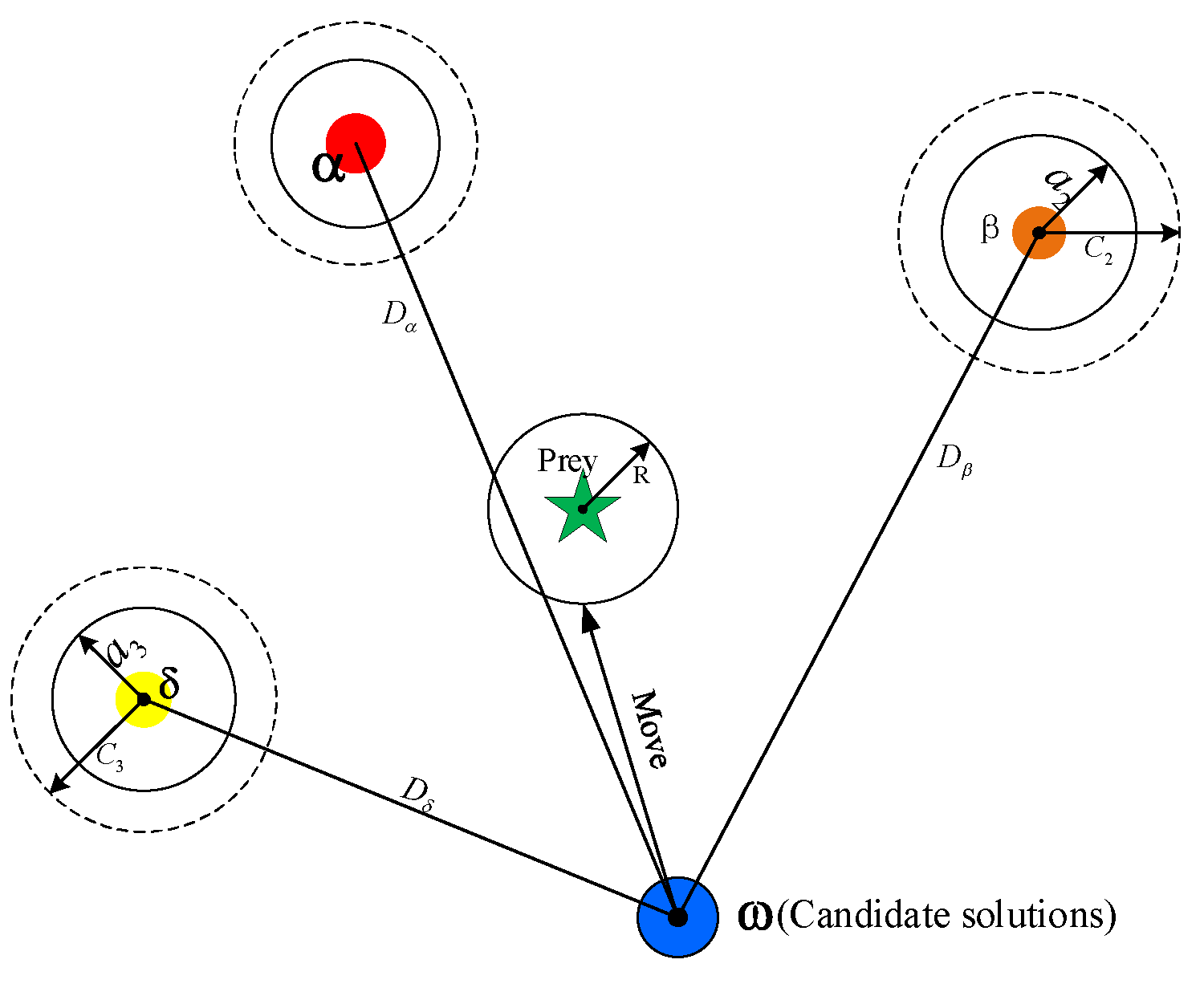
2.2.4. Parameter Optimization for LSSVM

The gray wolf optimizer (GWO) is an intelligent optimization algorithm that was developed as an optimized search method inspired by gray wolf predation activities. It has been widely considered by scholars for its strong convergence performance, few parameters, and easy realization and has been commonly applied to parameter optimization, image classification, and other fields [36,37]. Given the advantages of the GWO, we used the GWO optimization method to optimize parameters of regularization parameters γ and Gaussian kernel parameters σ for the LSSVM prediction model in this study.
The GWO optimization algorithm simulates the predation behavior of wolves, including the processes of social hierarchy, encircling, and attacking prey. The gray wolf group is divided into four social hierarchies from the highest to the lowest, including the head wolf (or dominant wolf) α , which is mainly responsible for making decisions on the activities of wolves and has the strongest management ability. Other wolves should follow their orders; the β wolf obeys α wolves; the δ wolf, obeying the α and β wolf, controls the remaining levels. The ω wolf, at the bottom of the class, is subject to the decision-making of the wolves of all other social levels.
(1). Mathematical description. For the GWO model, α is the optimal solution, β and δ are the suboptimal solutions, and ω is the candidate solution. The GWO optimization process is mainly guided by α , β , and δ whereas ω just follows them to track, surround, and attack the prey.
(2). Encircling Prey. When gray wolves search for prey, they will gradually approach and surround the prey and then keep iterating on this process, leading to the globally optimal solution. The update formulas for wolf predation position are described briefly below:
D = | C · X p ( t ) X ( t ) |
X ( t + 1 ) = X p ( t ) A · D
A = 2 a · r 1 a
C = 2 · r 2
where t represents the present iteration. D is the distance between the gray wolves and the corresponding prey. X ( t ) is the position of the wolf. Correspondingly X p ( t ) is the position of prey. A and C is the coefficient vector of synergy. a is the linear decline parameter, decreasing from 2 to 0 at each iteration. r1 and r2 are the random vectors ranging from 0 to 1, respectively.
(3). Hunting Prey. Gray wolves can identify the location of potential prey (the optimal solution), and the search process is mainly completed by the guidance of α , β , and δ ; however, the spatial characteristics for the solution of many problems are unknown, and the gray wolf is unable to determine the exact location of the optimal solution. α , β , and δ in the current population were kept, then the direction of movement towards the prey was determined according to their position information. The positions of α , β , δ , and ω were updated and adjusted. The first three optimal values of the history are preserved during the iteration process, and other individuals in the population constantly update their positions through the location of the optimal value. The following is the mathematical representation of the gray wolves hunting procedure:
D α = | C 1 · X α ( t ) X ( t ) |
D β = | C 2 · X β ( t ) X ( t ) |
D δ = | C 3 · X δ ( t ) X ( t ) |
X 1 = X α A 1 · D α
X 2 = X β A 2 · D β
X 3 = X δ A 3 · D δ
X ( t + 1 ) = X 1 + X 2 + X 3 3
where X α , X β , and X δ represent the position vector of α , β , and δ , respectively, at the present iteration. D α , D β , D δ are the distance vectors between ω and α , β , and δ , respectively, at the present iteration. X 1 , X 2 , and X 3 are the location updating procedure under the leadership of α , β , and δ , respectively. A is the convergence factor. When | A | > 1 , wolves scatter in search of the target, allowing the GWO to perform global searches; when | A | < 1 , the wolves concentrate their search on the target. C is also a random vector. Figure 1 depicts the gray wolf update search location.
(4). Attacking Prey. The purpose is to capture the target, that is, to complete the GWO. According to Equation (28), the decrease in the value of a will cause the value of A to fluctuate accordingly and A [ 1 , 1 ] .

3. Highway Traffic Flow Forecasting Model

3.1. The Proposed Highway Traffic Flow Prediction Model

In the study, we established an improved hybrid model based on the CEEMDAN and LSSVM methods to predict highway traffic flow. The core of the prediction method is decomposition and prediction. First, the original traffic flow time series is decomposed by the CEEMDAN method into a certain number of time-series components from high to low frequency, and then these components are reorganized according to IWPE. Prediction models are constructed for these recombined components, and the prediction results are combined as the final traffic flow forecast result. Figure 2 shows the structure of the proposed model. The specific implementation steps are described as follows.
Step 1. Original data decomposition. The original nonstationary highway traffic flow data collected per 5-min intervals is decomposed by the CEEMDAN method, and K IMF components and a residual component R(t) are obtained. The CEEMDAN method overcomes modal aliasing and reduces the difficulty and complexity of expressway short-term traffic flow data prediction. The decomposed components are simpler than the original traffic flow data. The error obtained by predicting the decomposed components is smaller than the original number, and the complexity is not so high.
Step 2. Subsequences reorganization. Entropy can describe the complexity of the time series. In this paper, the permutation entropy is improved to obtain an improved weighted permutation entropy. Through calculating the IWPE of each component, the complexity of each subsequence is obtained. Then the sequences with similar IWPE are combined to form a new component, which reduces the number of components and avoids repeated calculations, thereby reducing the amount of calculation in the prediction stage.
Step 3. Traffic flow prediction. The LSSVM model components are used for prediction. The regularization parameters of LSSVM and Gaussian kernel function parameters determine the effect of the prediction model; therefore, we use the GWO optimization algorithm to improve the LSSVM. To minimize RMSE of the prediction result, finding the optimal parameter combination avoids artificial selection of parameters, thereby improving the prediction accuracy. Finally, the traffic flow prediction results are added together to obtain the final prediction result.

3.2. Performance Criteria

In the study, we used three important evaluation criteria to measure the performance of the prediction model: mean absolute error (MAE), root mean square error (RMSE), and equilibrium coefficient (EC).
(1) MAE
The value range of MAE is [0, +∞). When the prediction value is the same as the actual data, it is equal to 0, indicating that the established model is perfect. The greater the error between the true data and predicted result, the greater the value.
MAE = 1 N i = 1 N | y ^ i y i |
(2) RMSE
The value range of RMSE is [0, +∞). When the prediction value is the same as the actual data, it is equal to 0, indicating that the established model is perfect. The greater the error between the true data and prediction result, the greater the value.
RMSE = 1 N i = 1 N ( y ^ i y i ) 2
(3) EC
EC represents the fitting degree. EC > 0.85 means the prediction effect is good; EC > 0.9 means that the prediction effect is very good. The following is the calculation formula:
EC = 1 i = 1 N ( y ^ i y i ) 2 i = 1 N y i 2 + i = 1 N y ^ i 2

4. Experimental Verification

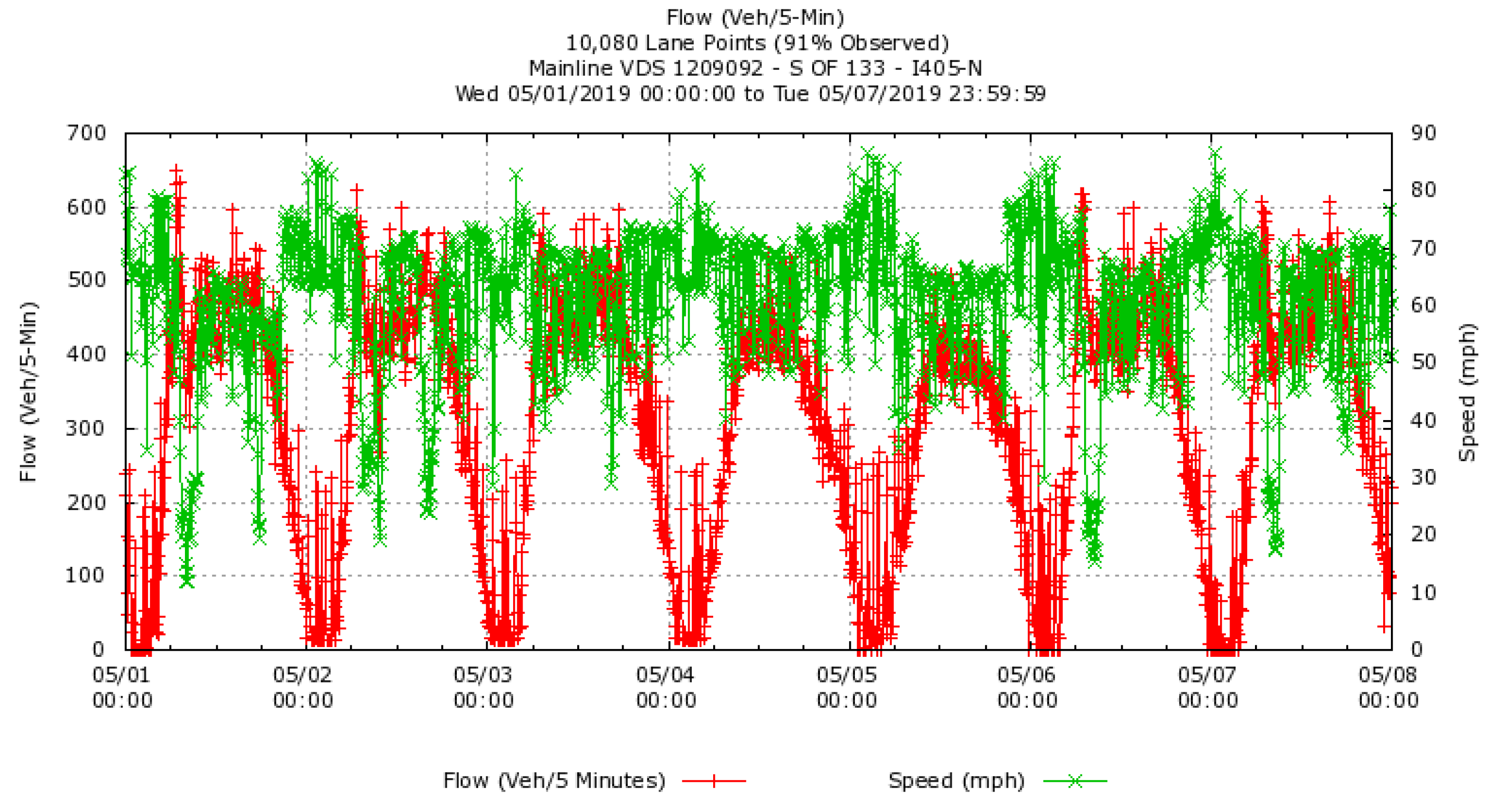
4.1. Experimental Data Description

Extensive experiments were performed to quantitatively verify the performance of our proposed method. For this study, we adopted the data from the California Department of Transportation Caltrans Performance Measurement System (PeMS) collected from the detector no. VDS-1209092 on I405-N freeway in the City of Irvine [38]. The PeMS can collect, filter, process, aggregate, and examine traffic data in real-time. We used the datasets collected from 1 May to 7 May 2019, per 5-min interval, containing information such as traffic flow, speed, and occupancy rate, for a total of 2016 data points to train and modify the prediction models. The datasets were divided into two parts. The first part (1 May 2019 to 5 May 2019) was used as training data to train the proposed model. The second part, from 6 May 2019 to 7 May 2019, was used to adjust the model parameters. Then, we used the trained model to predict the traffic flow of 8 May 2019, and the predicted value was compared with the actual value of 8 May 2019. Figure 3 illustrates the data collection location and relevant details. Figure 4 reveals the raw traffic flow and speed data from 1 May to 7 May 2019.

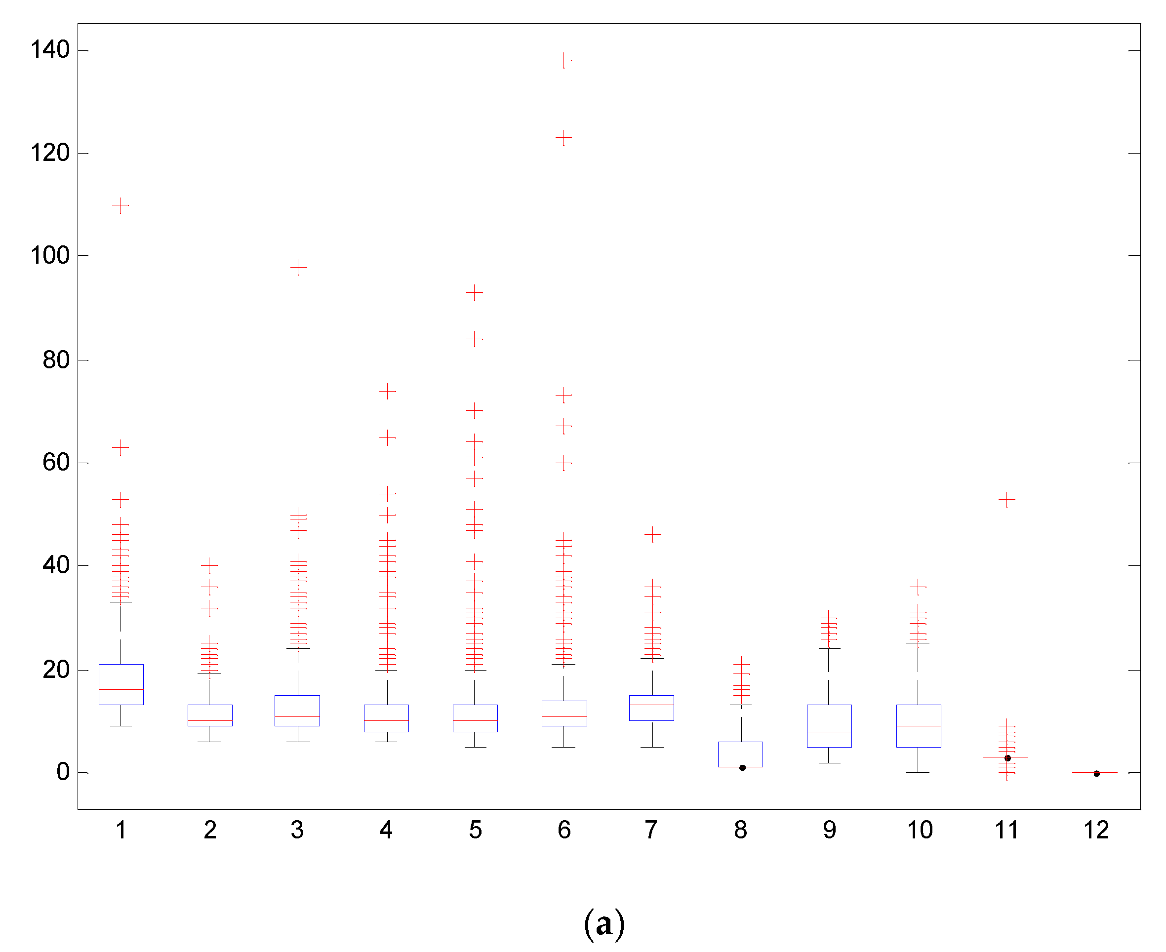
4.2. Traffic Flow Time-Series Decomposition and Reconstruction with the CEEMDAN-IWPE Method

The CEEMDAN decomposition method was used to decompose the highway traffic flow data. Figure 5 shows the decomposition results. The CEEMDAN method can decompose the traffic flow data into 12 subsequences, including 11 IMF components, and 1 residual component. To highlight the performance of CEEMDAN, both EMD and EEMD methods were used to process the same traffic flow data. Figure 6 and show the decomposition results of the EMD and EEMD methods, respectively. Figure 6 shows that the EMD model decomposes the road traffic flow into 11 subsequences, including 10 IMFs, and 1 residual. Similarly, Figure 7 shows that EEMD decomposes the road traffic flow into 12 subsequences, including 11 IMFs, and a residual. The results indicate that the EMD, EEMD, and CEEMDAN models can effectively decompose the complex original highway traffic flow data sequence into a certain number of components from high frequency to low frequency. It is worth noting that each IMF component decomposed by the CEEMDAN method is relatively independent, and the mode mixing phenomenon has been significantly improved. At the same time, Figure 8a–c show the iterations for realizing each IMF component of CEEMDAN, EEMD, and EMD methods.
If we directly establish prediction models for all components decomposed by CEEMDAN, multiple errors will be introduced into the models, thus, the final prediction error will increase, the prediction will be inaccurate, and the calculation time will increase; therefore, to reduce the prediction error and calculation cost, we used the IWPE method proposed in Section 2 to calculate the IWPE value of IMFs and reconstruct the components.
When calculating each IMF component’s IWPE, it is necessary to reconstruct the phase space of each IMF component separately. In the process of time series phase space reconstruction, we used the classical C-C method to determine the two important parameters of phase space reconstruction, namely the delay parametric and the embedded dimension. According to the C-C method, the delay time τ is the time corresponding to the first local minimum, and the relationship between embedding dimension d and delay time τ is τ ω = ( d 1 ) τ , where τ ω is the time corresponding to the global minimum. Figure 9 shows the relationship between the delay time τ and the embedded dimension d of each IMF component time series decomposed by CEEMDAN. Table 1 shows the τ , d , and the IWPE value for each IMF component.
Figure 10 shows the IWPE values of all components. The IWPE value of the IMF component obtained by CEEMDAN decomposition reduces with the decrease of the IMF frequency, which shows that it is effective to measure the complexity and randomness of the IMF component by using the IWPE method. Then, we reorganize the IMF according to the IWPE value of each IMF component and merge the IMF components with similar IWPE values into a new subsequence. In this way, the number of components is greatly reduced, thereby reducing the computational complexity and time overhead of the prediction phase. In Figure 10, the subsequences IWPE value of IMF1, IMF2, IMF3, IMF4, and IMF5 are similar, and the differences are small, so they can be merged, integrated, and reconstructed into a new subsequence, named IMFr 1, to input into the GWO-LSSVM for training and forecasting. The IWPE values of IMF8 and IMF9 are similar, thus IMF8 and IMF9 can be combined into a new sequence. The IWPE values of IMF6, IMF7, IMF10, IMF11, and residual are quite different and remain their original values. After the reconstruction is completed, the number of subsequences is reduced from 12 to 7. The reconstructed sequences are shown in Figure 11.

4.3. Highway Traffic Flow Forecasting Results and Analysis

4.3.1. Highway Traffic Flow Forecasting

After decomposing and reconstructing the original traffic flow time series, 7 GWO-LSSVM prediction models were constructed, and 7 subsequences were used to train and modify the models. After comparing and analyzing the kernel function for the LSSVM model, we decided to use the Gaussian kernel function as the kernel function. The GWO algorithm was used to optimize the two parameters of LSSVM to obtain the optimal parameter combination. The minimum RMSE index was selected as the optimization target. The relationship between the number of iterations and the fitness value in the optimization process is shown in Figure 12. We set the maximum number of iterations to 10; after 7 iterations, the objective function value tends to flatten to the minimum. Finally, we found that the regularization parameter was 88.49, and the Gaussian kernel parameter was 1.74. The final prediction result is shown in Figure 13. Figure 13 suggests that the predicted value is almost the same as the actual value with a small error. The MAE is 0.92, and the RMSE is 1.22, indicating that the proposed prediction model can effectively predict traffic flow.

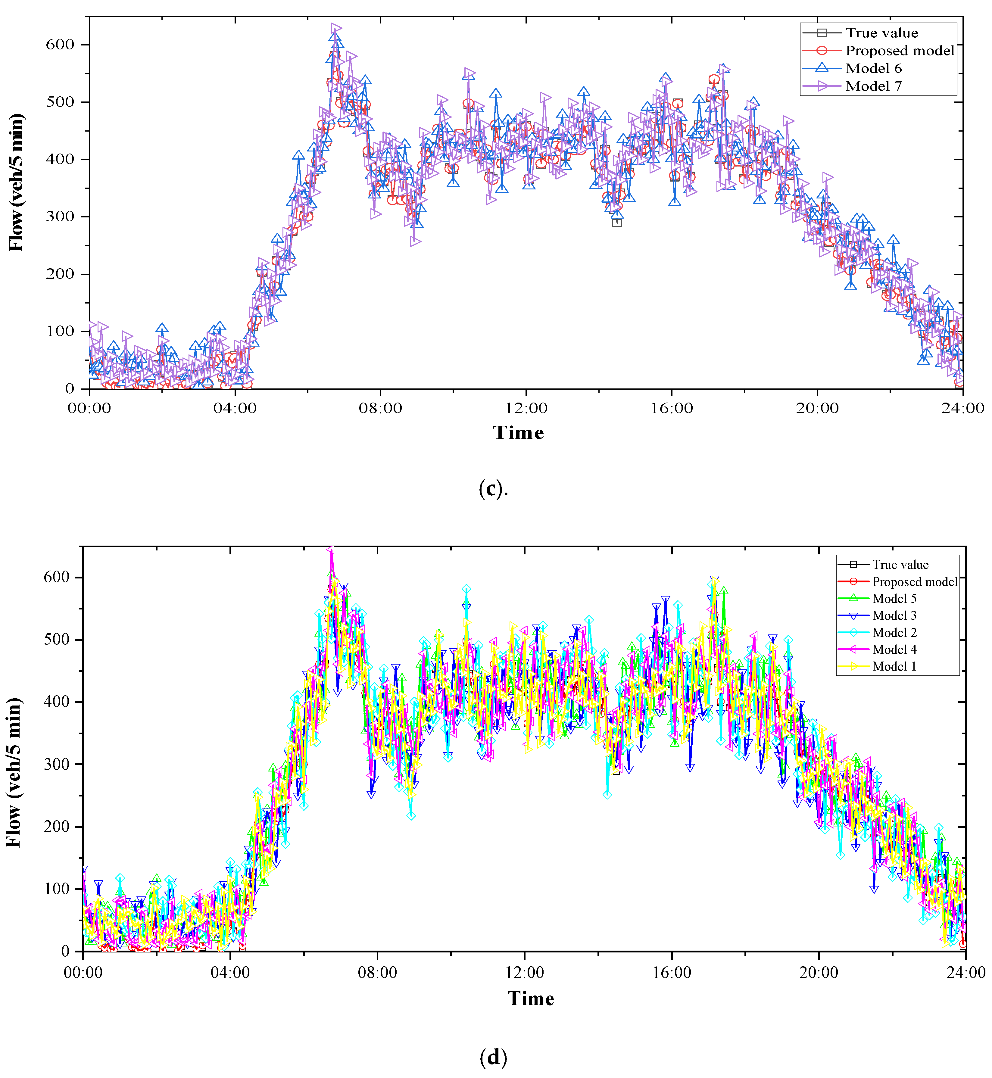
4.3.2. Comparison Models

To confirm the performance and superiority of the proposed hybrid prediction model (i.e., a hybrid of CEEMDAN with IWPE for raw traffic data decomposition and GWO optimized LSSVM for prediction, abbreviated as CEEMDAN-IWPE-LSSVM-GWO), the same highway traffic flow experimental data were employed for modeling. A total of 12 alternative forecasting models were constructed for comparative analysis with the proposed hybrid model. Table 2 shows the instructions of comparison models in detail.
Figure 14 and Table 3 show that the calculations of MAE, RMSE, and EC of the proposed model are the best, and its forecasting accuracy is the highest. The detailed analysis and discussion are as follows.
(1). In Figure 14a, we compare Model 9 to the proposed model (CEEMDAN-PE-GWO-LSSVM), which shows that the MAE and RMSE of the proposed model are improved by 37.77% and 44.01%, respectively. The results show that the improved weighted permutation entropy can reduce the error more effectively and is the most effective model in the data processing stage. This is because, in the process of IMF component reconstruction, the weighted permutation entropy (IWPE), which can comprehensively measure the complexity of IMF components, has a better processing effect than the PE method. Comparing Model 8 (CEEMDAN-IWPE-LSSVM) to the proposed model, the MAE and RMSE of the latter are improved by 75.39% and 75.40%, respectively, more than two times as much as the former compared to the CEEMDAN-IWPE-GWO-LSSVM model, which indicates that the GWO-optimized LSSVM model can greatly increase prediction precision. Since the training process of the LSSVM involves the adjustment of many parameters by the GWO method, the forecasting accuracy of this model is further improved after systematic parameter optimization.
(2). In Figure 14b, we compare Model 10 (CEEMDAN-IWPE-BP), Model 11 (CEEMDAN-IWPE-SVM), and Model 12 (CEEMDAN-IWPE-ARIMA) to the proposed model, respectively: the prediction effect of the proposed model is significantly better than Model 10, Model 11, and Model 12. The evaluation indexes of the proposed model are the best, and its forecasting accuracy is the highest. This suggests that the LSSVM has higher accuracy than the BP, SVM, and ARIMA models and has broad application prospects in highway traffic flow prediction.
(3). In Figure 14c, we compare Model 6 (EMD-IWPE-LSSVM-GWO) and Model 7 (EEMD-IWPE-LSSVM-GWO) with the proposed model, respectively: the value of MAE reduced from 19.8924 and 21.0938 to 1.9167, and the value of RMSE reduced from 24.5237 and 25.4538 to 2.2623. The forecasting effect of the proposed model is greatly improved, and the forecasting error is reduced. The apparent improvement indicates that the fluctuation of traffic flow forecasting results obtained by the CEEMDAN method is smoother, and it can reduce the nonlinearity and forecasting errors of the raw dataset.
(4). In Figure 14d, we compare Model 1 (LSSVM), Model 2 (BP), Model 3 (SVM), Model 4 (ARIMA), and Model 5 (LSSVM-GWO) with the proposed model, respectively: the prediction effect of the proposed model is greatly improved, and the forecasting error is reduced. The results suggest that the original traffic flow data through decomposition and prediction is significantly better than the direct prediction without data decomposition.
In Table 3, we rank the prediction effects of the proposed model and comparison model from highest to lowest as follows: the proposed model, Model 9, Model 8, Model 10, Model 11, Model 12, Model 6, Model 7, Model 5, Model 1, Model 3, Model 2, and Model 4. This illustrates that, if the original traffic flow data were processed to a certain extent, no matter what decomposition method is used, the performance would be better than that of direct prediction without decomposition. The EC value of the proposed model is the highest, up to 0.992, indicating that the proposed prediction model can highly fit and predict the trend of future traffic flow.

5. Conclusions

In this paper, we proposed an improved hybrid model of CEEMDAN with IWPE for raw traffic data decomposition and GWO-optimized LSSVM for short-term highway traffic flow prediction. The proposed method first uses the CEEMDAN method to decompose the original traffic flow time-series data into a certain number of IMF components. Since training and building a prediction model for each IMF component in the prediction stage will increase the computational cost and amount of calculation, a method for reconstructing IMF components was proposed. The IWPE of each IMF time-series component instead of permutation entropy was calculated after phase space reconstruction, and then IMF components with similar entropy values were combined to obtain recombined components. Next, the prediction model was established. The LSSVM prediction model was adopted for prediction. We introduced the GWO optimization algorithm to optimize the important parameters of the LSSVM model, which avoided the artificial selection of parameters and improved prediction accuracy. The proposed method was tested on the collected data through California’s Freeway Performance Measurement System and compared with several other models. By analyzing the prediction results of different comparison models, we showed that the model proposed in this paper is superior to other prediction models in three aspects: 1. The CEEMDAN model was used to process and predict the original data, which reduced the prediction error; 2. The proposed IWPE can make up for PE defects while considering the numerical value and the permutation position of time series; and 3. The GWO method was used to optimize LSSVM parameters and can improve prediction accuracy. In future studies, we plan to study a highway traffic flow prediction method that takes space, weather, accidents, and other factors into consideration.

Author Contributions

Conceptualization and investigation, X.W. and S.L.; resources and data curation, Z.W. and M.Z.; formal analysis, methodology, writing—original draft, writing—review & editing, and Validation, R.C. All authors have read and agreed to the published version of the manuscript.

Funding

This research was funded by National Natural Science Foundation of China, grant number 61873109.

Conflicts of Interest

The authors declare no conflict of interest.

References

  1. Zhang, D.; Kabuka, M.R. Combining weather condition data to predict traffic flow: A GRU-based deep learning approach. IET Intell. Transp. Syst. 2018, 12, 578–585. [Google Scholar] [CrossRef]
  2. Djenouri, Y.; Belhadi, A.; Lin, J.C.W.; Cano, A. Adapted K-Nearest Neighbors for Detecting Anomalies on Spatio-Temporal Traffic Flow. IEEE Access 2019, 7, 10015–10027. [Google Scholar] [CrossRef]
  3. Yang, S.X.; Ji, Y.; Zhang, D.; Fu, J. Equilibrium between Road Traffic Congestion and Low-Carbon Economy: A Case Study from Beijing, China. Sustainability 2019, 11, 219. [Google Scholar] [CrossRef] [Green Version]
  4. Zhang, W.B.; Han, G.J.; Wang, X.; Guizani, M.; Fan, K.G.; Shu, L. A Node Location Algorithm Based on Node Movement Prediction in Underwater Acoustic Sensor Networks. IEEE Trans. Veh. Technol. 2020, 69, 3166–3178. [Google Scholar] [CrossRef]
  5. Ramezani, M.; Ye, E. Lane density optimisation of automated vehicles for highway congestion control. Transp. B 2019, 7, 1096–1116. [Google Scholar] [CrossRef]
  6. Li, Z.C.; Huang, J.L. How to Mitigate Traffic Congestion Based on Improved Ant Colony Algorithm: A Case Study of a Congested Old Area of a Metropolis. Sustainability 2019, 11, 1140. [Google Scholar] [CrossRef] [Green Version]
  7. Alesiani, F.; Moreira-Matias, L.; Faizrahnemoon, M. On Learning from Inaccurate and Incomplete Traffic Flow Data. IEEE Trans. Intell. Transp. Syst. 2018, 19, 3698–3708. [Google Scholar] [CrossRef]
  8. Tanveer, M.; Kashmiri, F.A.; Naeem, H.; Yan, H.M.; Qi, X.; Rizvi, S.M.A.; Wang, T.S.; Lu, H.P. An Assessment of Age and Gender Characteristics of Mixed Traffic with Autonomous and Manual Vehicles: A Cellular Automata Approach. Sustainability 2020, 12, 2922. [Google Scholar] [CrossRef] [Green Version]
  9. de Luca, S.; Di Pace, R.; Memoli, S.; Pariota, L. Sustainable Traffic Management in an Urban Area: An Integrated Framework for Real-Time Traffic Control and Route Guidance Design. Sustainability 2020, 12, 726. [Google Scholar] [CrossRef] [Green Version]
  10. Rojo, M. Evaluation of Traffic Assignment Models through Simulation. Sustainability 2020, 12, 5536. [Google Scholar] [CrossRef]
  11. Williams, B.M. Modeling and Forecasting Vehicular Traffic Flow as a Seasonal Stochastic Time Series Process; University of Virginia: Charlottesville, VA, USA, 1999. [Google Scholar]
  12. Jomnonkwao, S.; Uttra, S.; Ratanavaraha, V. Forecasting Road Traffic Deaths in Thailand: Applications of Time-Series, Curve Estimation, Multiple Linear Regression, and Path Analysis Models. Sustainability 2020, 12, 395. [Google Scholar] [CrossRef] [Green Version]
  13. Okutani, I.; Stephanedes, Y.J. Dynamic Prediction of Traffic Volume Through Kalman Filtering Theory. Transp. Res. B-Meth. 1984, 18, 1–11. [Google Scholar] [CrossRef]
  14. Emami, A.; Sarvi, M.; Bagloee, S.A. Short-term traffic flow prediction based on faded memory Kalman Filter fusing data from connected vehicles and Bluetooth sensors. Simul. Model. Pract. Theory 2020, 102, 102025. [Google Scholar] [CrossRef]
  15. Cai, L.R.; Zhang, Z.C.; Yang, J.J.; Yu, Y.D.; Zhou, T.; Qin, J. A noise-immune Kalman filter for short-term traffic flow forecasting. Phys. A 2019, 536, 122601. [Google Scholar] [CrossRef]
  16. Frazier, C.; Kockelman, K.M. Chaos theory and transportation systems—Instructive example. Stat. Methods Saf. Data Anal. Eval. 2004, 1897, 9–17. [Google Scholar] [CrossRef] [Green Version]
  17. Adewumi, A.; Kagamba, J.; Alochukwu, A. Application of Chaos Theory in the Prediction of Motorised Traffic Flows on Urban Networks. Math. Probl. Eng. 2016, 2016, 5656734. [Google Scholar] [CrossRef] [Green Version]
  18. Castro-Neto, M.; Jeong, Y.S.; Jeong, M.K.; Han, L.D. Online-SVR for short-term traffic flow prediction under typical and atypical traffic conditions. Expert Syst Appl. 2009, 36, 6164–6173. [Google Scholar] [CrossRef]
  19. Dimitriou, L.; Tsekeris, T.; Stathopoulos, A. Adaptive hybrid fuzzy rule-based system approach for modeling and predicting urban traffic flow. Transp. Res. C-Emerg. Techonol. 2008, 16, 554–573. [Google Scholar] [CrossRef]
  20. El-Sayed, H.; Sankar, S.; Daraghmi, Y.A.; Tiwari, P.; Rattagan, E.; Mohanty, M.; Puthal, D.; Prasad, M. Accurate Traffic Flow Prediction in Heterogeneous Vehicular Networks in an Intelligent Transport System Using a Supervised Non-Parametric Classifier. Sensors 2018, 18, 1696. [Google Scholar] [CrossRef] [PubMed] [Green Version]
  21. Bratsas, C.; Koupidis, K.; Salanova, J.M.; Giannakopoulos, K.; Kaloudis, A.; Aifadopoulou, G. A Comparison of Machine Learning Methods for the Prediction of Traffic Speed in Urban Places. Sustainability 2020, 12, 142. [Google Scholar] [CrossRef] [Green Version]
  22. Cai, L.R.; Chen, Q.; Cai, W.H.; Xu, X.M.; Zhou, T.; Qin, J. SVRGSA: A hybrid learning based model for short-term traffic flow forecasting. IET Intell. Transp. Syst. 2019, 13, 1348–1355. [Google Scholar] [CrossRef]
  23. Wang, Y.P.; Zhao, L.N.; Li, S.Q.; Wen, X.Y.; Xiong, Y. Short Term Traffic Flow Prediction of Urban Road Using Time Varying Filtering Based Empirical Mode Decomposition. Appl. Sci. 2020, 10, 238. [Google Scholar] [CrossRef] [Green Version]
  24. Luo, C.; Huang, C.; Cao, J.D.; Lu, J.Q.; Huang, W.; Guo, J.H.; Wei, Y. Short-Term Traffic Flow Prediction Based on Least Square Support Vector Machine with Hybrid Optimization Algorithm. Neural Process. Lett. 2019, 50, 2305–2322. [Google Scholar] [CrossRef]
  25. Chen, X.B.; Cai, X.W.; Liang, J.; Liu, Q.C. Ensemble Learning Multiple LSSVR With Improved Harmony Search Algorithm for Short-Term Traffic Flow Forecasting. IEEE Access 2018, 6, 9347–9357. [Google Scholar] [CrossRef]
  26. Mackenzie, J.; Roddick, J.F.; Zito, R. An Evaluation of HTM and LSTM for Short-Term Arterial Traffic Flow Prediction. IEEE Trans. Intell. Transp. Syst. 2019, 20, 1847–1857. [Google Scholar] [CrossRef]
  27. Liu, H.; Wang, J. Vulnerability Assessment for Cascading Failure in the Highway Traffic System. Sustainability 2018, 10, 2333. [Google Scholar] [CrossRef] [Green Version]
  28. Mena-Oreja, J.; Gozalvez, J. A Comprehensive Evaluation of Deep Learning-Based Techniques for Traffic Prediction. IEEE Access 2020, 8, 91188–91212. [Google Scholar] [CrossRef]
  29. Huang, N.E.; Zheng, S.; Long, S.R.; Wu, M.C.; Shih, H.H.; Quanan, Z.; Yen, N.-C.; Tung, C.C.; Liu, H.H. The Empirical Mode Decomposition and the Hilbert Spectrum for Nonlinear and Non-Stationary Time Series Analysis. Proc. R. Soc. Lond. Ser. A Math. Phys. Eng. Sci. 1998, 454, 903–995. [Google Scholar] [CrossRef]
  30. Huang, N.E.; Wu, M.L.C.; Long, S.R.; Shen, S.S.P.; Qu, W.D.; Gloersen, P.; Fan, K.L. A confidence limit for the empirical mode decomposition and Hilbert spectral analysis. Proc. R. Soc. Lond. Ser. A Math. Phys. Eng. Sci. 2003, 459, 2317–2345. [Google Scholar] [CrossRef]
  31. Wu, Z.; Huang, N.E. Ensemble Empirical Mode Decomposition: A Noise-Assisted Data Analysis Method. Adv. Adapt. Data Anal. 2011, 1, 1–41. [Google Scholar] [CrossRef]
  32. Yeh, J.-R.; Shieh, J.-S.; Huang, N.E. Complementary Ensemble Empirical Mode Decomposition: A Novel Noise Enhanced Data Analysis Method. Adv. Adapt. Data Anal. 2011, 2, 135–156. [Google Scholar] [CrossRef]
  33. Huo, Z.Q.; Zhang, Y.; Jombo, G.; Shu, L. Adaptive Multiscale Weighted Permutation Entropy for Rolling Bearing Fault Diagnosis. IEEE Access 2020, 8, 87529–87540. [Google Scholar] [CrossRef]
  34. Suykens, J.A.K.; Vandewalle, J. Least squares support vector machine classifiers. Neural Process. Lett. 1999, 9, 293–300. [Google Scholar] [CrossRef]
  35. Cortes, C.; Vapnik, V.N. Support Vector Networks. Machine Learn. 1995, 20, 273–297. [Google Scholar] [CrossRef]
  36. Mirjalili, S.; Mirjalili, S.M.; Lewis, A. Grey Wolf Optimizer. Adv. Eng. Softw. 2014, 69, 46–61. [Google Scholar] [CrossRef] [Green Version]
  37. Al-Tashi, Q.; Abdulkadir, S.J.; Rais, H.M.; Mirjalili, S.; Alhussian, H.; Ragab, M.G.; Alqushaibi, A. Binary Multi-Objective Grey Wolf Optimizer for Feature Selection in Classification. IEEE Access 2020, 8, 106247–106263. [Google Scholar] [CrossRef]
  38. Caltrans Performance Measurement System. Available online: http://pems.dot.ca.gov/ (accessed on 8 May 2020).
Figure 1. The gray wolf position update process for hunting prey.
Sustainability 12 08298 g001
Figure 2. The overall framework of the proposed highway traffic flow prediction model. CEEMDAN: complete ensemble empirical mode decomposition with adaptive noise; LSSVM: least-squares support vector machine; GWO: gray wolf optimizer.
Sustainability 12 08298 g002
Figure 3. The I405-N freeway position location of observation loop detector No.VDS-1209092 in the California Department of Transportation Caltrans Performance Measurement System (PeMS): (a) the I405-N freeway position location; (b) the location of loop detector No.VDS-1209092.
Sustainability 12 08298 g003
Figure 4. The raw traffic flow and speed of VDS-1209092 per 5-min interval from 1 May to 7 May 2019.
Sustainability 12 08298 g004
Figure 5. The results of the complete ensemble empirical mode decomposition with adaptive noise (CEEMDAN) method.
Sustainability 12 08298 g005
Figure 6. The results of the ensemble empirical mode decomposition (EEMD) method.
Sustainability 12 08298 g006
Figure 7. The results of the short-term highway traffic flow decomposed by the empirical mode decomposition (EMD) model.
Sustainability 12 08298 g007
Figure 8. The iterations for realizing each intrinsic mode function (IMF) component: (a) the iterations of CEEMDAN; (b) the iterations of EEMD; (c) the iterations of EMD.
Sustainability 12 08298 g008aSustainability 12 08298 g008b
Figure 9. The relationship between the delay time τ and the embedded dimension d of each IMF component using the C–C method.
Sustainability 12 08298 g009
Figure 10. The IWPE calculation results of each IMF component.
Sustainability 12 08298 g010
Figure 11. The reconstructed IMFr subsequences based on the IWPE method.
Sustainability 12 08298 g011
Figure 12. Iteration curve.
Sustainability 12 08298 g012
Figure 13. Highway traffic flow forecasting results based on the proposed model.
Sustainability 12 08298 g013
Figure 14. The comparison of the comparison models with the proposed model: (a) the comparison of the Model 8 and Model 9 with the proposed model; (b) the comparison of the Model 10, Model 11 and Model 12 with the proposed model; (c) the comparison of the Model 6 and Model 7 with the proposed model; (d) the comparison of the Model 1, Model 2, Model 3, Model 4 and Model 5 with the proposed model.
Sustainability 12 08298 g014aSustainability 12 08298 g014b
Table 1. The parameters τ, d, and improved weighted permutation entropy (IWPE) value calculated for each IMF component.
ComponentτdPEIWPE ValueNormalized IWPE
IMF1671.319621.189670.18082
IMF2481.306111.189890.18086
IMF32371.315031.188810.18069
IMF44131.317131.181440.17957
IMF5861.276131.168500.17760
IMF61081.023111.034490.15724
IMF71890.882030.926090.14076
IMF820110.522790.591460.08990
IMF93170.490140.597230.09077
IMF1012100.318550.417800.06353
IMF1116120.162180.308830.04694
RES2010.002030.001200.00001
Table 2. The instructions of comparison models. PE: permutation entropy.
ModelModel InstructionAbbreviation
proposed modela hybrid model of CEEMDAN with IWPE for raw traffic data decomposition and GWO optimized LSSVM for predictionCEEMDAN-IWPE-LSSVM-GWO
Model 1Least-squares support vector machine modelLSSVM
Model 2Back-propagation neural network modelBP
Model 3Support vector machine modelSVM
Model 4Autoregression moving average modelARIMA
Model 5GWO-optimized LSSVM modelLSSVM-GWO
Model 6a hybrid model of EMD with IWPE and GWO-optimized LSSVMEMD-IWPE-LSSVM-GWO
Model 7a hybrid model of EEMD with IWPE and GWO-optimized LSSVMEEMD-IWPE-LSSVM-GWO
Model 8a hybrid model of CEEMDAN with IWPE and LSSVMCEEMDAN-IWPE-LSSVM
Model 9a hybrid model of CEEMDAN with PE and GWO optimized LSSVMCEEMDAN-PE-LSSVM-GWO
Model 10a hybrid model of CEEMDAN with IWPE and BPCEEMDAN-IWPE-BP
Model 11a hybrid model of CEEMDAN with IWPE and SVMCEEMDAN-IWPE-SVM
Model 12a hybrid model of CEEMDAN with IWPE and ARIMACEEMDAN-IWPE-ARIMA
Table 3. Model performance for traffic flow prediction.
Forecasting ModelMAERMSEECRank
Proposed model1.91672.26230.9921
Model 122.454228.15920.91910
Model 224.695832.14450.90712
Model 323.543829.75310.91411
Model 426.076431.44620.87513
Model 521.369426.66980.9329
Model 619.892424.52370.9467
Model 721.093825.45380.9418
Model 87.78829.19560.9813
Model 93.07994.04120.9842
Model 1012.319414.80030.9784
Model 1113.562515.70540.9665
Model 1214.395818.73540.9536

