Article

Mapping Annual Land Use and Land Cover Changes in the Yangtze Estuary Region Using an Object-Based Classification Framework and Landsat Time Series Data

1
Faculty of Geomatics, East China University of Technology, Nanchang 330013, China
2
Shanghai Key Lab for Urban Ecological Processes and Eco-Restoration, East China Normal University, Shanghai 200241, China
3
Key Laboratory of the Causes and Control of Atmospheric Pollution of Jiangxi Province, East China University of Technology, Nanchang 330013, China
*
Author to whom correspondence should be addressed.
Sustainability 2020, 12(2), 659; https://doi.org/10.3390/su12020659
Submission received: 20 December 2019 / Revised: 10 January 2020 / Accepted: 13 January 2020 / Published: 16 January 2020

Abstract

:
A system understanding of the patterns, causes, and trends of long-term land use and land cover (LULC) change at the regional scale is essential for policy makers to address the growing challenges of local sustainability and global climate change. However, it still remains a challenge for estuarine and coastal regions due to the lack of appropriate approaches to consistently generate accurate and long-term LULC maps. In this work, an object-based classification framework was designed to mapping annual LULC changes in the Yangtze River estuary region from 1985–2016 using Landsat time series data. Characteristics of the inter-annual changes of LULC was then analyzed. The results showed that the object-based classification framework could accurately produce annual time series of LULC maps with overall accuracies over 86% for all single-year classifications. Results also indicated that the annual LULC maps enabled the clear depiction of the long-term variability of LULC and could be used to monitor the gradual changes that would not be observed using bi-temporal or sparse time series maps. Specifically, the impervious area rapidly increased from 6.42% to 22.55% of the total land area from 1985 to 2016, whereas the cropland area dramatically decreased from 80.61% to 55.44%. In contrast to the area of forest and grassland, which almost tripled, the area of inland water remained consistent from 1985 to 2008 and slightly increased from 2008 to 2016. However, the area of coastal marshes and barren tidal flats varied with large fluctuations.

1. Introduction

Estuaries are the interfaces between marine, freshwater, and terrestrial ecosystems and are welcomed as intermediate transitional zones with various ecosystem service functions [1]. Affected by climate change and rapidly urbanization, the estuarine and coastal regions are facing with many degradation risks, such as wetland shrinking, environmental pollution and coastal erosion [2,3]. To alleviate these problems, long-term dense monitoring of land use and land cover (LULC) change is of crucial important, because it provides essential information for depicting the history, current situation and future of LULC change, and for understanding biogeochemical processes and the mechanisms of LULC changes [4,5].
Remote sensing have been widely applied for mapping LULC over a variety of spatiotemporal scales in estuarine and coastal regions [6,7,8]. However, the choice of remotely sensed data for long-term dense and large-scale LULC mapping is usually a compromise between temporal frequency and spatial resolution [9]. LULC maps derived from high-spatial-resolution imagery (such as the Chinese satellite Gaofen-6 of imagery) provide fine detailed information, but the cost is expensive for frequent observation over large estuarine region. LULC maps derived from coarse resolution imagery (such as EOS-MODIS/NOAA-AVRHH data) have high temporal frequency and large coverage, but its spatial resolution is too coarse to track detail change of LULC [5]. Against this background, Landsat data with 16 days temporal resolution and 30 m spatial resolution, which provides the longest and most systematic historical data [10], is potentially more suitable than other data sources for monitoring dense LULC dynamics at large estuarine regions.
Many researchers have applied bi-temporal or sparse time series remotely sensed data to map and monitor LULC changes in estuarine and coastal regions [11,12,13,14]. For example, Kesgin and Nurlu [15] used a time series of Landsat TM and ASTER images to assess LULC change in the coastal zone of Candarli Bay, Turkey. However, most of the existing studies focused on the comparison of two points rather than depicting the entire record at once. They cannot separate gradual changes from sudden change, and represent a major obstacle for understanding how and why estuarine system change [16].
In terms of classification algorithms, LULC mapping can be performed by pixel-based and object-based methods. Pixel-based methods, such as random forest classifier and maximum likelihood algorithm, use the spectral information contained in individual pixels to map LULC classes. These methods are thoroughly exploit spectral information, and have been shown to achieve accurately for the mapping of certain LULC classes [17]. However, they are challenged to use the texture and context information, which cause low mapping accuracies in heterogeneous regions (such as estuary region) [18]. Luckily, new studies indicate that object-based approaches have great potential to map complex LULC landscape, and they are quickly gaining acceptance in remote sensing fields [19,20]. Compared to pixel-based approaches, object-based methods have several immediate benefits. First, the processing of units from pixels to image objects reduces both within-class spectral variation and “salt-and-pepper” effects, which are typical in pixel-based classification [21]. Second, a variety of features characterizing the spatial and contextual properties can be incorporated to the mapping procedures and improve mapping accuracy [22]. Third, it can be a close association between the boundaries of objects and their real-world counterparts [23].
Unsurprisingly, these advantages have resulted in, generally, higher mapping accuracies when compared to pixel-based methods [24,25]. For example, Tehrany et al. [26] assessed performance of object-based and pixel-based classification approaches for LULC mapping, the result showed that the object-based methods performed better than pixel-based methods. However, most of these researches focus on high or very high spatial resolution imagery. A few studies were found using long-term medium-spatial-resolution remote sensing data and object-based methods to monitor continuous LULC change. Thus, object-based mapping for long-term LULC change monitoring will continue to be a developing field.
For estuarine regions, these regions have complex heterogeneous landscape, and exhibit complex spectral characteristics. There has several challenges to generate appropriate time-series data to support long-term LULC monitoring [27]. The first challenge is a lack of robustness classification algorithm for long-term LULC mapping. The main reason is that Steep environmental gradients and highly dynamics in estuarine regions often alter land surface’s reflectance, and that make it difficult to use only one algorithm to accurately map long-term LULC change in these regions [28]. The second challenge is that selecting training samples for the classification of historical images is difficult. One reason is that the accessibility to high-spatial-resolution remotely sensed data is limited and the associated costs of acquiring and processing are very high [29]. Another reason is that in situ historical data is usually lacking, especially in estuarine regions [30]. The third challenge is data gaps due to cloud contamination in estuarine and coastal regions [31]. This makes it difficult to map long-term dense LULC products. Thus, approaches for consistent classification of image time series urgently need to develop for monitoring long-term LULC changes in estuarine and coastal regions.
In this study, a typical estuarine and coastal region, namely the Yangtze River estuary, was selected as the study area to explore these challenges. The Yangtze River estuary, one of the most famous estuaries in the world, is an ecologically and economically important region, which provides a wide range of ecosystem services, such as habitat for coastal vegetation and animals, carbon sequestration, and food supply [1,2]. With rapid urbanization and accelerated climate change, the LULC pattern in the study area has underwent unprecedented changes in past decades. Previous studies have shown that the high rate of LULC conversion in this area have created a series of environmental problems, such as coastal wetland degradation, water pollution and biodiversity loss [32]. Unfortunately, due to the lack of a system understanding of long-term LULC changes, the dynamic linkages between LULC changes and its environmental responses are poorly understood. Therefore, it is of the utmost importance for the mapping and monitoring of long-term LULC to optimize management strategies.
In this work, to explore ways to solve the challenges mentioned above, an object-based classification framework was developed to mapping long-term LULC dynamics of the Yangtze River estuary region using annual time-series of Landsat data. The specific goal is (1) to develop an object-based framework for generating consistent annual Landsat time series LULC maps by integrating four of prevailing LULC mapping techniques (object-based image analysis, hierarchical classification, and updating and backdating approaches) and (2) to quantify and assess annual LULC change in the Yangtze River estuary region from 1985 to 2016.

2. Materials and Methods

2.1. Study Area

The Yangtze River estuary, one of the most famous coastal and estuarine ecoregions in the world, was selected as the study area. The region is located in East China, and the study area includes the Shanghai municipality and portions of Suzhou and Nantong in Jiangsu Province. The estuary extends from 30°33′ to 32°8′ N in latitude and from 120°50′ to 122°7′ E in longitude, covering an area of 13929.75 km2 (Figure 1). Topographically, the region is composed of plains, except for a few hills located in the southwest. The climate is a marine subtropical monsoon climate, where clouds are frequent during the entire year. The region covers complex urban impervious materials, cropland, forest, water body and grass, as well as a variety of wetlands. However, the Yangtze River estuary has become a vulnerable region due to intense human activities and uncertain climate change.

2.2. Landsat Image Preprocessing

A consistent Landsat data preprocessing process was developed to process all the Landsat images. The process included atmospheric correction, image co-registration, poor-quality observation detection, gap filling, mosaicking and data clipping. Landsat TM (Landsat Thematic Mapper)/ETM+ (Landsat Enhanced Thematic Mapper Plus) bands 1–5 and 7 and bands 2–7 for Landsat OLI (Landsat 8 Operational Land Imager) were used in this work.

2.2.1. Image Selection

The Landsat images used in this study were acquired from the United States Geological Survey (USGS, http://glovis.usgs.gov/). All Landsat data covering the study area were assessed from 1984 to 2016. Two issues were considered in selecting high-quality images (Table 1): (1) the cloud contamination of a selected image was < 10% (mainland cover parts) as much as possible in the study area; (2) the selected images should cover the three key growing seasons of natural vegetation in each year to improve the classification accuracy [33]. These seasons include the early growing season (“spring,” March to May), peak growing season (“summer,” June to September), and late growing season (“autumn,” October to December). However, due to cloud contamination, cloud-free images were not available for some years during all three key phenological phases. Thus, images of adjacent years were used as alternatives. In addition, one scene at the lowest tide for each year was selected for tidal flat extraction (Table 1).

2.2.2. Atmospheric Correction and Geometric Correction

For all selected Landsat images, the Fast Line of Sight Atmospheric Analysis of Spectral Hypercubes (FLAASH) algorithm was chosen to perform atmospheric corrections, which can accurately correct the radiation errors caused by various reasons [34]. All images were geometrically registered into a UTM projection (zone 51, North) with geometric errors of less than one pixel. Thus, all images have the same coordinate system.

2.2.3. Gap Filling and Cloud Removal

The failure of the Scan Line Corrector (SLC) on Landsat 7’s ETM+ sensor in 2003, caused to approximately 22% of the pixels per scene not being scanned. The SLC failure has reduced the capacity of those images for mapping LULC dynamics. Thus, methods for gap filling were needed to address the missing values before image consequent processing. The gap-filling approach developed by Garcia [35] was used to solve the missing values in this study. This method is a three-dimensional spatiotemporal interpolation algorithm. The algorithm is a penalized least-squares regression based on a three-dimensional discrete cosine transform. It can maintain the original signal where data exist and minimize smoothing effects where new data are interpolated [36]. This algorithm has been successfully applied in previous studies [37]. Compared with the existing gap-filling methods [38], Garcia’s method did not require ancillary data to simulate the missing pixel values and can accurately restore the values of unscanned pixels.
In this study, clouds and cloud shadows were visually detected and removed through the assembly of cloud-free observations from multi-temporal imagery of the same year.

2.2.4. Calculation of Spectral Indices

Several spectral indices were selected for LULC mapping in this study: the Enhanced Vegetation Index (EVI) [39], Modified Normalized Difference Water Index (MNDWI) [40], and Normalized Difference Build-Up Index (NDBI) [41]. The EVI was used to separate vegetation types from not-vegetation types, the MNDWI was used to extract water; and impervious and pervious surfaces were mapped with the NDBI. To minimize classification errors due to phenological differences, the effect of individual precipitation events and image temporal differences [42], the average EVI (EVIave), the average MNDWI (MNDWIave), and the average NDBI (NDBIave) were calculated. These spectral indices were calculated using the Landsat surface reflectance based on the following equations and spectral bands:
EVI   =   2.5 × ( ρ NIR     ρ RED ) / ( ρ NIR   +   6   ×   ρ RED     7.5   ×   ρ BLUE   +   1.5 ) ,
MNDWI   = ( ρ GREEN     ρ SWIR 1 ) / ( ρ GREEN   +   ρ SWIR 1 ) ,
NDBI   = ( ρ SWIR 1     ρ NIR ) / ( ρ SWIR 1   +   ρ NIR ) ,
EVI ave   =   ( EVI spring   +   EVI summer + EVI autumn ) / 3 ,
MNDWI ave   =   ( MNDWI spring   +   MNDWI summer   +   MNDWI autumn ) / 3 ,
NDBI ave   =   ( NDBI spring   +   NDBI summer   +   NDBI autumn ) / 3 ,
where ρ BLUE , ρ GREEN ,   ρ RED ,   ρ NIR ,   and   ρ SWIR 1 are the surface reflectance values of the blue band, green band, red band, near infrared band, and shortwave infrared band (band 6 for Landsat OLI, band 5 for Landsat TM/ETM+), respectively.

2.3. Classification Scheme

Based on the research aims, features of the acquired images and field surveys, a nine-class scheme was designed for the study area (Table 2) based on a modified version of the scheme proposed by Gong et al. [43].

2.4. Object-Based Classification Framework

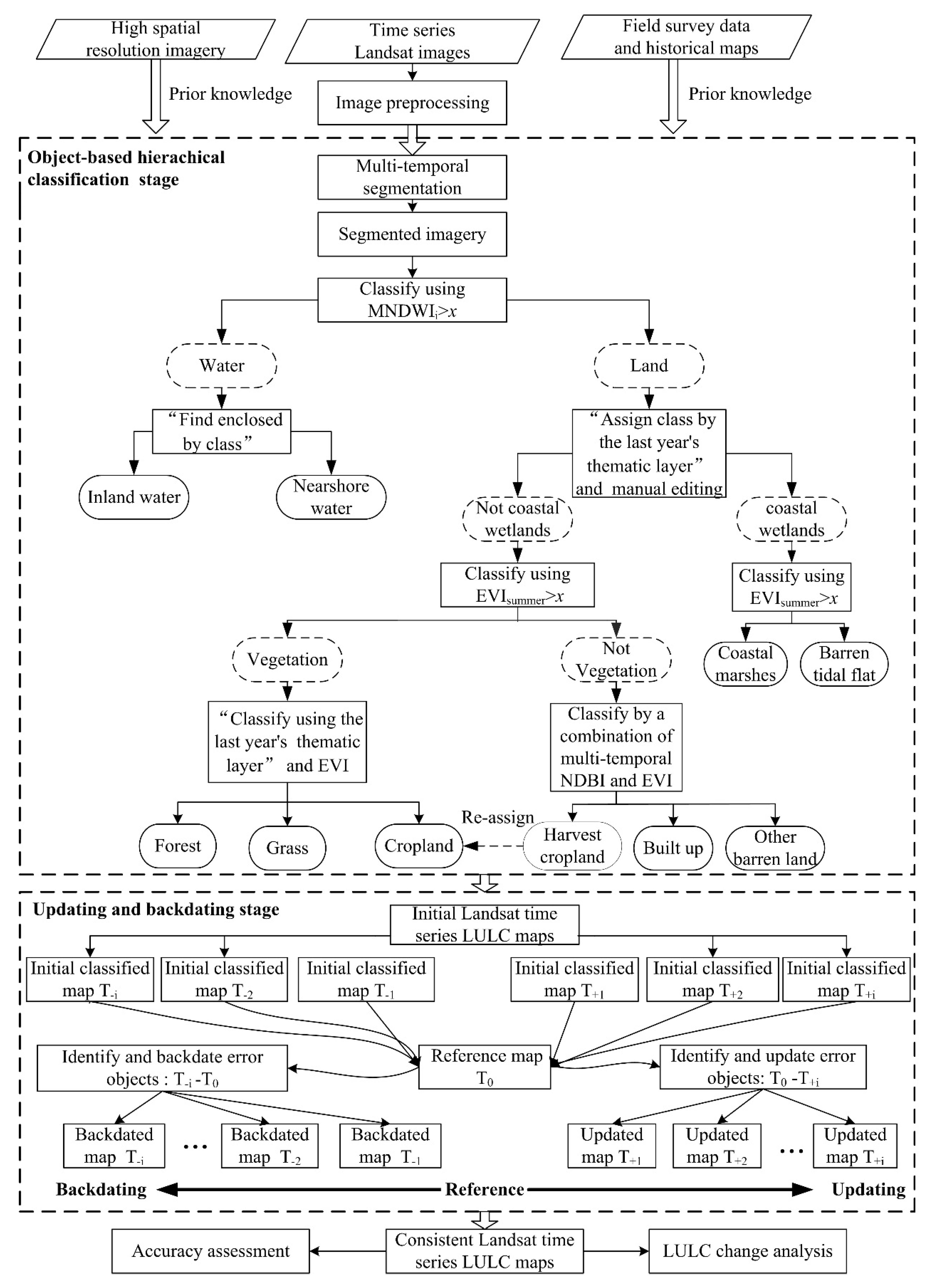
An object-based framework was designed to integrate object-based image analysis, hierarchical classification, updating and backdating approaches for LULC mapping in this study, as shown in Figure 2. In the framework, multi-temporal imagery was first segmented to generate image objects. Then, a rule-based hierarchical classification method was implemented to generate the initial LULC maps. In this stage, lots of prior knowledge obtained from field survey data and historical maps, such as spectral characteristics, phonological metrics, and spatial features for each class, was incorporated into the rule-based classifier to improve the classification accuracy. Trial and error methods are used to select the classification parameters and determine the optimal threshold values to classify each types, but this approach may increase the chance for classification inconsistencies. To overcome these issues, updating and backdating approaches were used to reduce the misclassification errors and generate more consistent LULC maps. After these steps, an accuracy assessment was performed for the LULC products. Finally, time series LULC products were used for change analysis.

2.5. Multi-Temporal Segmentation

In this study, image segmentation was implemented in eCognition® Developer 8.7 software. The multiresolution segmentation algorithm was selected as the image segmentation algorithm, which was proposed by Baatz and Schäpe [44]. The algorithm merges pixels based on a heterogeneity criterion, which can be adjusted by selecting the scale parameter, weights of spectral bands, spectral factor, and compactness factor [45,46]. Following Drǎguţ et al. [47], the ESP tool was used to aid in determining appropriate parameter settings for image segmentation. To guarantee the homogeneity of objects across the 32 years of Landsat time series, all time-series images were processed using the same parameters that were sufficiently detailed to map all the LULC classes in this study. Namely, multi-temporal images (“spring,” “summer,” and “autumn”) were segmented in each year using 18 bands with equal weighting, a shape parameter of 0.1, compactness of 0.6, and scale factor of 20.

2.6. LULC Classification

2.6.1. Object-Based Hierarchical Classification Stage

After image segmentation, an object-based hierarchical classification approach was implemented to generate the initial LULC products. An overview of the LULC mapping rule set is shown in Figure 2. In Figure 2, four steps are applied in the rule set. In the first step, water was extracted using the MNDWI. Considering the seasonal variations of water bodies, the summer images were used as reference images because summer is the rainy season in the study area. In the second step, a hybrid method was used within each land class to separate “coastal wetlands” from “not coastal wetlands.” The algorithm named “assign class by thematic layer” within eCognition was first used to extract the ‘coastal wetlands’, of which the input vector was the coastal wetland layer from the previous year. The final “coastal wetland” boundaries were modified by visual interpretation. In the water category, the algorithm named “find enclosed by class” within eCognition was used to separate inland water and nearshore water. In the third step, within the “not coastal wetlands” class, “vegetation” was separated from “not vegetation” using EVIsummer. Within the “coastal wetlands,” coastal marshes were distinguished from barren tidal flats using EVIsummer. In the final step, within the “not vegetation” type, harvest cropland was separated from the other two categories through analysis of the multi-temporal EVI and NDBI. Notably, high EVI and low NDBI values were obtained when harvest cropland was in the replantation phase. Built-up land was separated from other barren land using the NDBI. Within the vegetation category, a method similar to that adopted to classify “coastal wetlands” was applied to separate forest and grass from cropland.

2.6.2. Updating and Backdating Stage

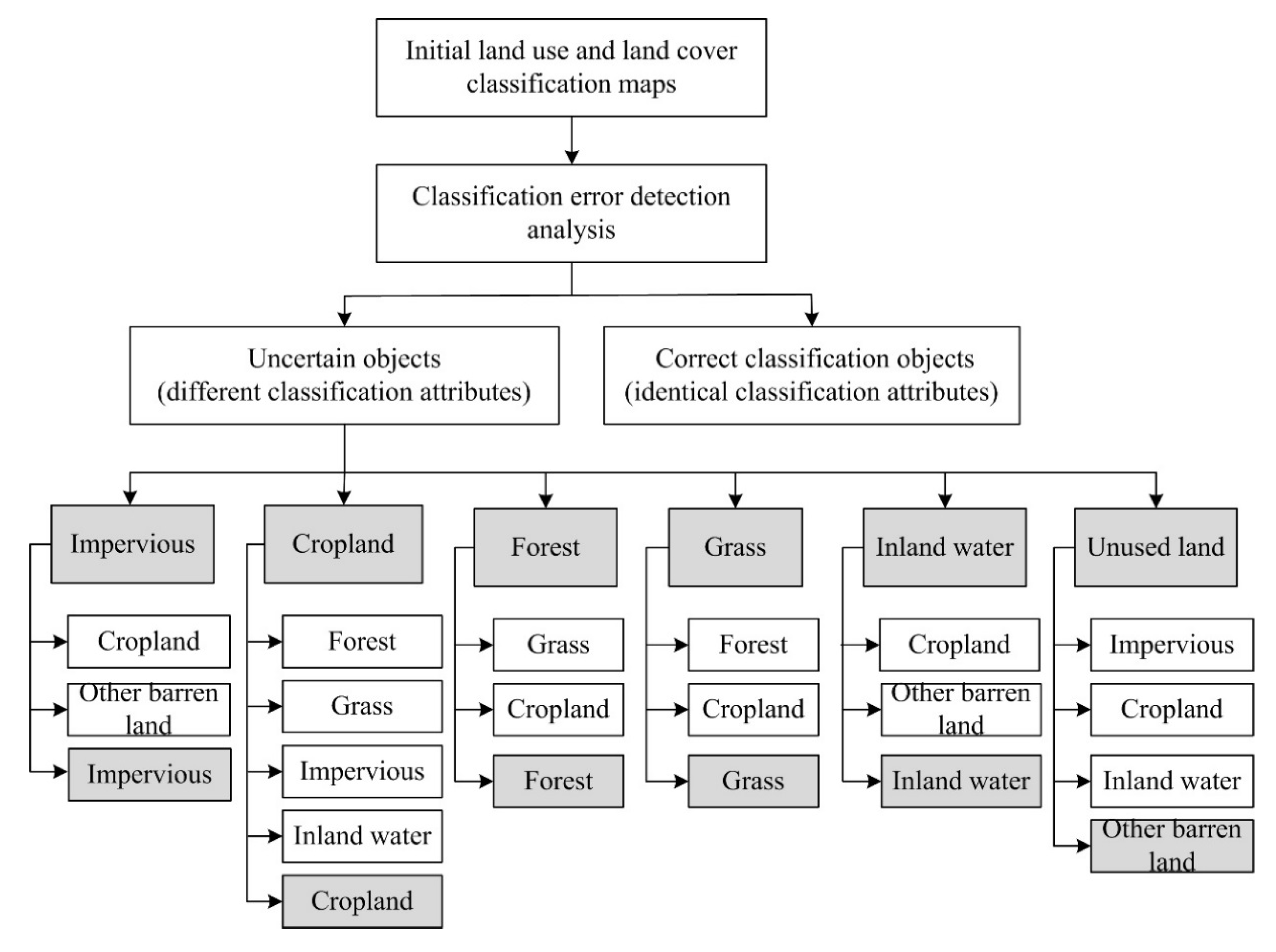
After hierarchical classification, error analysis showed that a certain amount of error could still be observed in the initial classified maps. To reduce these errors, updating and backdating approaches were used to generate more accurate LULC products (Figure 2). In this stage, classification error detection analysis was implemented, and 15 major misclassification scenarios occurred (Figure 3) (for coastal marshes, barren tidal flats and nearshore water, good classification results were achieved from the previous stage, so these three classes did not require updating/backdating). To perform updating/backdating, the overlay analysis method was first used to determine “correct classification objects” and “uncertain objects.” Objects with identical classification types (attributes) between the reference map (T0) (Table 1) and the initial classified map (Ti) were assigned as “correct classification objects.” Objects with different classification types between Ti and T0 were labeled as “uncertain objects.”
As shown in Figure 3, the “correct classification objects” maintained the original classified results when performing updating/backdating. Among the “uncertain objects,” only the misclassified objects required updating/backdating for classification correction, and the remaining “uncertain objects” maintained the original classified results (Figure 3). A combination of rule-based methods and a visual interpretation approach was used to identify and reclassify the misclassified objects from the “uncertain objects” (Table 3). The visual interpretation approach of updating/backdating error objects was used through manual editing of the initial classified layer. The rule-based approach is a semi-automatic reclassified process. For example, if one misclassification object requires an update to impervious land, two criteria must be met: (a) the attribute of the object in T0 must be impervious, and (b) the values of EVIave and NDBIave in Ti must be less than 0.2 and greater than −0.1, respectively. In this stage, the works of Yu et al., Linke and McDermid. and Linke et al. are recommended as references for understanding more details of updating and backdating methods [48,49,50]. The reference maps used in this stage were generated by visual interpretation of the initial classified maps based on multi-temporal Landsat imagery and Google Earth maps.

2.7. Accuracy Assessment

Orthorectified aerial photos, high-resolution imagery from Google Earth, and field survey data were combined to produce reference data. Since available historical high-resolution imagery cannot cover the whole study area for the period from 1985 to 1998, reference data were also created from multi-temporal Landsat imagery and historical maps through visual interpretation in those period. The method proposed by Cochran was used to determine the total sample size [51]. Once the total sample size was determined, the approach proposed by Olofsson et al. [52] was used to determine the allocation of samples for specific categories. Namely, we allocated 50 samples per rare class (forest, grass, coastal marshes and unused land), and a sample size of n-200 was then proportionally allocated to the remaining classes. Accordingly, we used a random sampling scheme to generate the checkpoints for each class. Because the accuracy assessment required very intensive visual analysis and long-term time series and high spatial resolution data were not all available in this study, accuracy assessments were only conducted for the LULC maps from 1985, 1992, 1998, 2005, 2011, and 2016. The sampling design scheme of this study is shown in Table 4. Accuracy was assessed using a confusion matrix to calculate the overall accuracies, user’s and producer’s accuracies, and the Kappa coefficient [53].

3. Results

3.1. Accuracy Assessment of the LULC Maps

An accuracy assessment of the LULC products indicated that the map accuracies from the object-based classification framework approach were high (Supplementary Table S1). The overall accuracies (OA) were 87.82%, 87.43%, 85.77%, 86.30%, 86.74%, and 87.85% in 1985, 1992, 1998, 2005, 2011, and 2016, respectively, and the Kappa coefficients were 0.77, 0.78, 0.76, 0.78, 0.79, and 0.82, respectively. Cropland, inland water, coastal mashes and barren tidal flats were accurately classified, with user’s accuracies (UA) and producer’s accuracies (PA) of greater than 80% for all tested maps. For impervious cover, PA ranged from 77.63% to 87.21%, and UA ranged from 61.98% to 87.85%. The relatively low classification accuracy of impervious cover in 1985 and 1992 was mostly caused by low-density impervious regions. Such regions were often confused with cropland due to the limited spatial resolution and image quality. The rare LULC types, including forest, grass and other barren land, were relatively poorly classified, and the associated UAs were generally lower than 75%.

3.2. Long-Term LULC Dynamics

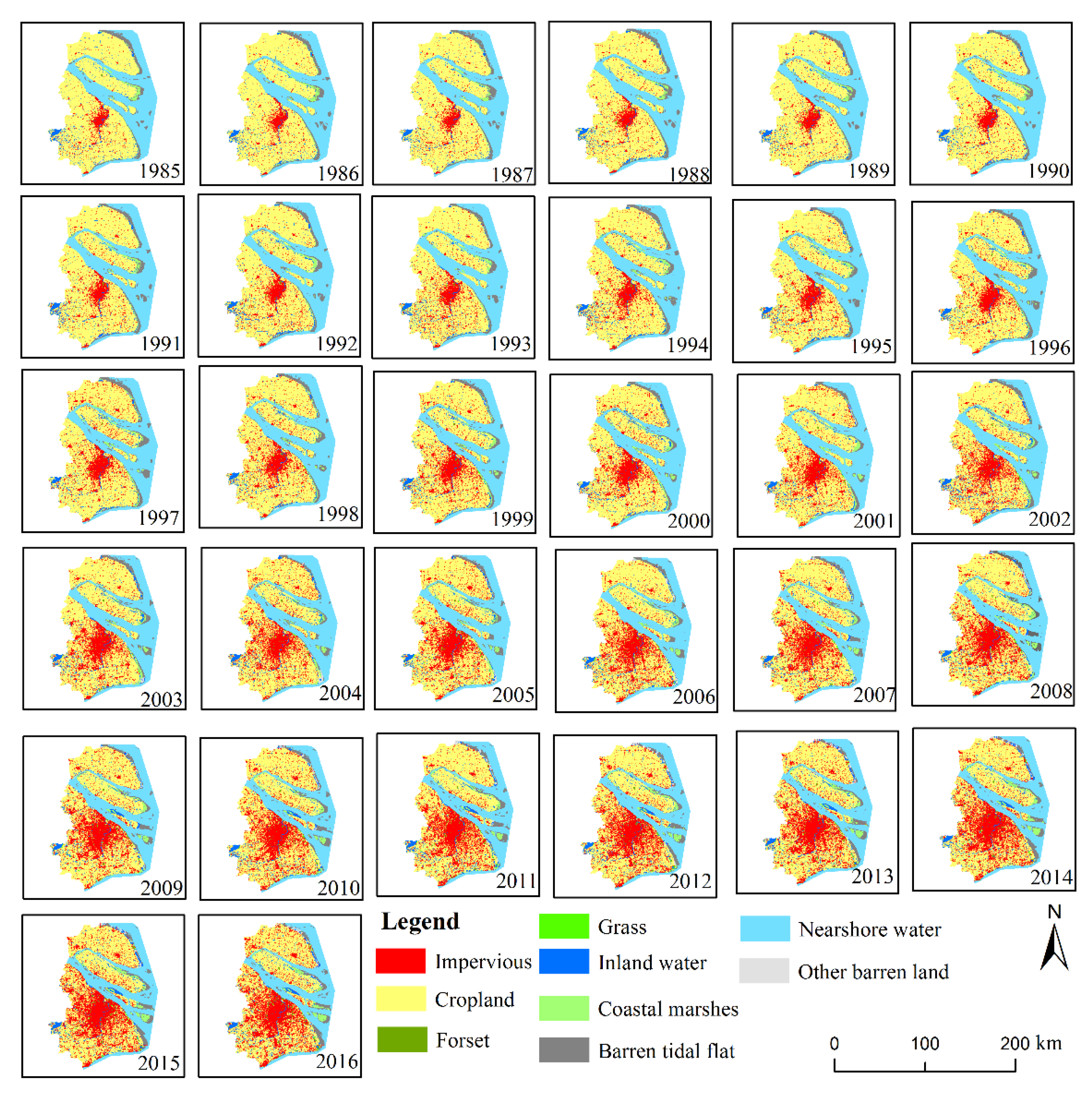
The spatial distributions of LULC types are clearly demonstrated in Figure 4, and the long-term changes are illustrated across each panel. The LULC classification results showed that great change was observed across the study area, especially change near the coastlines and peri-urban region. Specifically, cropland was the most extensive LULC type, but it continuously and rapidly decreased from 1985 to 2016. In contrast, impervious cover continuously and significantly expanded due to rapidly urbanization. Figure 4 also indicates that forest and grass substantially increased during the study period, although the proportions are still very small. The spatiotemporal distribution of coastal wetlands (including coastal marshes and barren tidal flats) varied and exhibited large fluctuations. Other barren land displayed an upward trend due to large-scale reclamation and the formation of increasing amounts of reclaimed lands from 2000 to 2016.
Quantitatively speaking, the land area of the study region increased by 730.13 km2 from 1985 to 2016, with an average annual increase of 23.55 km2. This increase was due to land reclaimed from coastal wetlands (coastal marshes, bare tidal flat and nearshore water). For specific categories, the cropland area continuously decreased from 8076.63 km2 (80.61%) in 1985 to 5959.33 km2 (55.44%) in 2016 (Figure 5), with an average annual decrease of 68.3 km2, and had a trend of continuous decrease (Slope = −65.96, R2 = 0.99). The impervious coverage increased from 642.84 km2 (6.42%) in 1985 to 3140.88 km2 (22.55%) in 2016, with an average annual increase of 80.58 km2, thus resulting in a trend to continuous increase (Slope = 80.95, R2= 0.99). This expansion was mainly at the expense of cropland. The area of forest and grass increased by more than triple the original area during this period due to the long-term implementation of urban greening. The proportion of inland water was stable from 1985 to 2008 and then experienced a slight increase from 2008 to 2016. The area of coastal marshes fluctuated. Barren tidal flat areas underwent continued declining trends due to long-term reclamation activities (Slope = −6.41, R2 = 0.55).

3.3. Monitoring Gradual Changes with Long-Term Time Series of LULC Products

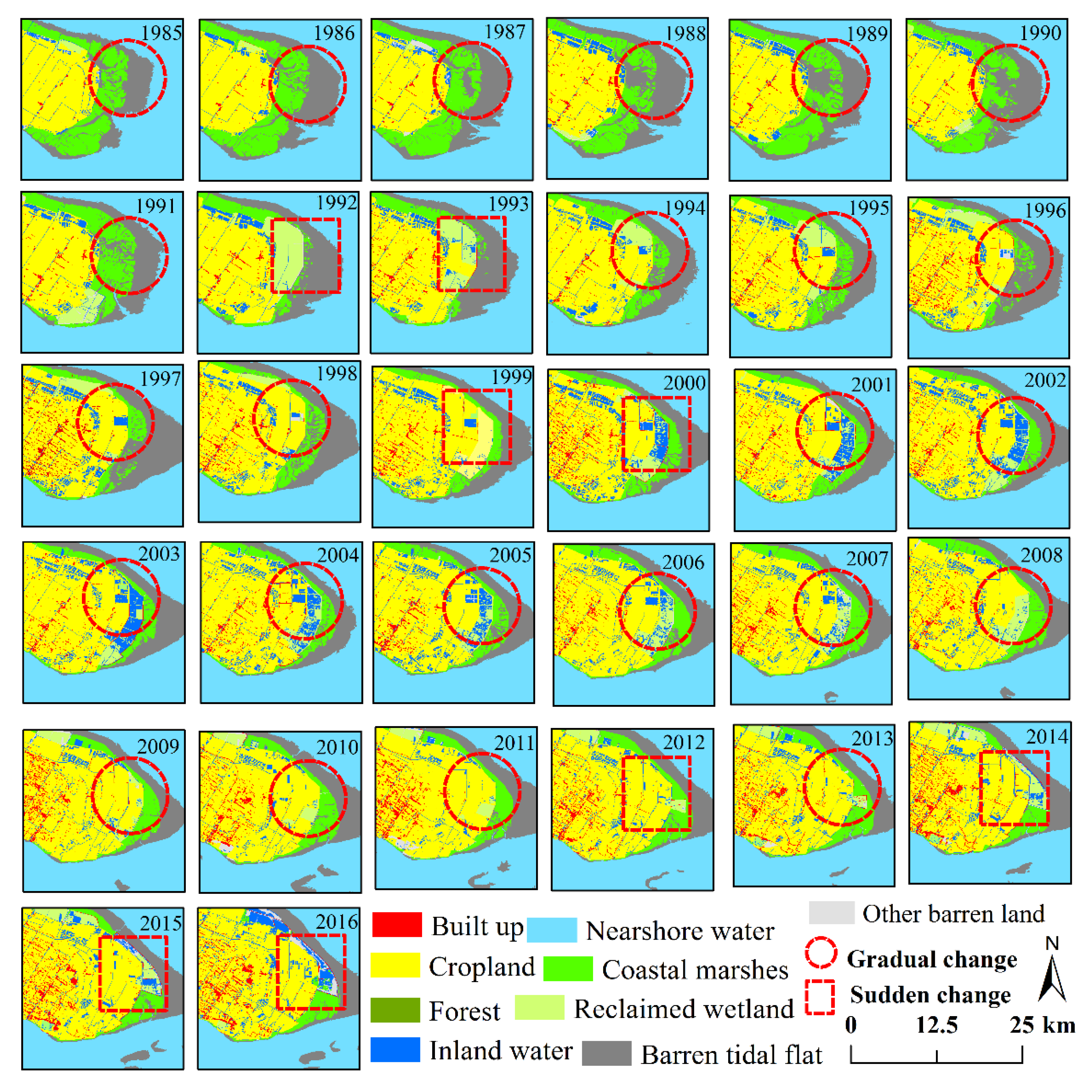
Compared with most previous studies that used bi-temporal or sparse time series images [28], this work contributed to the analysis of LULC changes by using annual, long-term Landsat time series data. With annual time series LULC maps, the long-term (including gradual changes) and short-term trends (e.g., sudden change) in LULC dynamics can be monitored. Figure 4 clearly reflects the continuous spatiotemporal process of LULC change in the Yangtze River estuary from a time series perspective. More importantly, gradual changes that would not be observed using bi-temporal or sparse time series maps can be detected with LULC products produced in this paper. Here, we consider LULC gradual changes to be those that are occurring over a period of several years or more, usually relating gradual LULC transitions over that time period. At a conceptual level, some of the most notable example of gradual change involve to LULC undergoing a gradual shift through time, such as the process of re-growing saltmarsh vegetation after damage by typhoon. To present the details of these gradual changes, the generated maps in a selected region (Chongming Dongtan wetland natural reserve) were enlarged and illustrated, as shown in Figure 6. Figure 6 not only shows the sudden change of coastal marshes by disease or natural disasters or large-scale reclamation (denoted by the red ellipse region in Figure 6) but also shows regrowth and long-term recovery from these events (denoted by the red rectangle and circle regions in Figure 6). It is difficult to map such gradual changes using bi-temporal or sparse time series maps.

4. Discussion

4.1. Advantages and Disadvantages of the Proposed Framework

In this study, an object-based classification framework was developed to generate a consistent Landsat time series for the long-term monitoring of LULC changes in the Yangtze River estuary region. This objective was completed through a combination of object-based image analysis, hierarchical classification, and updating and backdating approaches. Several advantages have been made to generate consistent long-term LULC maps in the proposed framework. First, compared to the traditional supervised classification algorithms [17], the proposed framework can make better use of spatial information such as shape and context, which can improve classification accuracy for complex LULC mapping. Second, compared to popular machine learning and deep learning algorithms, the proposed method does not need training samples, which is difficult to select training samples for these popular algorithms [54]. Third, object-based classification framework can largely reduce the errors caused by spatial misregistration, which is a common phenomenon and difficult to completely eliminate when using pix-based methods [55]. Finally, the proposed framework (updating and backdating stages) allow for a more straightforward utilization of prior knowledge. For example, the study area has not obviously appeared the phenomenon of counter-urbanization, thus we can use updating approach to improve the mapping accuracy of built up class (The classification result of reference image can be directly updated as the result of corresponding misclassified objects from the “uncertain objects”).
However, the approach has some disadvantages that must be addressed. Data gaps (due to cloud contamination and gap filling) and temporal difference problems in images are the main sources of classification error in this study, and novel methods, such as data fusion, should be introduced or proposed to address these problems. Another issue in the proposed method is related to the mixed pixel problem. Due to complex LULC types in estuarine and coastal regions, mixed pixels are very common and may result in the inaccurate estimation of LULC. Hence, sub-pixel analysis may be useful to overcome these mixed pixel problems in future studies. In addition, compared to LULC mapping, using a Google Earth Engine–like platform [56,57], the proposed method is still a time-consuming and laborious work.

4.2. Implications for Ecological Restoration

Under the combined effects of human activities and climate change, most of estuarine and coastal ecosystems are in a degraded state. Ecological restoration is widely used to reverse the degraded state. Understanding annual LULC changes is the first step to have some insight on ecological degeneration and conducting restoration projects. Analyzing a long-term time series of LULC products is critical for predicting further LULC changes in management of ecosystem services [16,23], which is important for decision making during the implementation of ecological restoration projects. Information provided by the annual LULC products can be used to assess restoration effects associated with ecosystem functions and services. On top of that, annual LULC products provide basic data for understanding the mechanisms and processes of ecosystem restoration.

5. Conclusions and Future Work

In summary, an object-based classification framework that integrates object-based image analysis, hierarchical classification, and updating and backdating approaches was developed for mapping long-term LULC changes in the Yangtze River estuary region from 1985–2016 using annual Landsat time series images. The results showed that the annual time series of LULC maps could clearly reflect the continuous spatiotemporal change process of LULC in the study area that would not have been observed using bi-temporal or sparse time series maps. The impervious area rapidly increased from 6.42% to 22.55% of the total land area from 1985 to 2016, and the cropland area dramatically decreased from 80.61% to 55.44%. Additionally, the area of forest and grass increased by more than three times the original area. The proportion of inland water remained stable from 1985 to 2008 and exhibited a slight increase from 2008 to 2016. The area of coastal marshes and barren tidal flats displayed fluctuating change, and barren tidal flats exhibited a rapidly decreasing trend. Furthermore, the time series of LULC products revealed gradual changes that are valuable for both ecological and environmental management. An accuracy assessment of single-year classifications indicated that the designed framework provides an efficient method with OAs of over 86%.This study also shows the limitations of the proposed framework such as not full automatic and mixed pixel problem. Further work will focus on the change mechanisms among different land cover classes and more robust and automatic classification algorithms require further development to map long-term LULC change.

Supplementary Materials

The following are available online at https://www.mdpi.com/2071-1050/12/2/659/s1, Table S1. Confusion matrix of land cover validation.

Author Contributions

Design, methodology, and data processing, J.A.; writing-original draft preparation, J.A., C.Z., L.C., and D.L. Funding acquisition, J.A. All authors have read and agreed to the published version of the manuscript.

Funding

This work was supported by the Open Research Fund of Shanghai Key Lab for Urban Ecological Processes and Eco-Restoration (SHUES2019A07), Doctoral Scientific Research Foundation of East China University of Technology (DHBK2018001), Major Projects of Shanghai Science and Technology Commission (18DZ1206506) and Shanghai Natural Science Foundation of China (No. 17ZR1427400). Sincere thanks are given for the comments and contributions of anonymous reviewers and members of the editorial team.

Acknowledgments

The authors would like to express their sincere thanks to Zhiqiang Gao for his guidance of this article. Sincere thanks are given for the comments and contributions of anonymous reviewers and members of the editorial team.

Conflicts of Interest

The authors declare no conflict of interest.

References

  1. Zhao, B.; Yan, Y.; Guo, H.; He, M.; Gu, Y.; Li, B. Monitoring rapid vegetation succession in estuarine wetland using time series MODIS-based indicators: An application in the Yangtze River Delta area. Ecol. Indic. 2009, 9, 346–356. [Google Scholar] [CrossRef]
  2. Tian, B.; Wu, W.; Yang, Z.; Zhou, Y. Drivers, trends, and potential impacts of long-term coastal reclamation in China from 1985 to 2010. Estuar. Coast. Shelf Sci. 2016, 170, 83–90. [Google Scholar] [CrossRef]
  3. Ai, J.; Gao, W.; Gao, Z.; Shi, R.; Zhang, C. Phenology-based Spartina alterniflora mapping in coastal wetland of the Yangtze Estuary using time series of GaoFen satellite no. 1 wide field of view imagery. J. Appl. Remote Sens. 2017, 11, 026020. [Google Scholar] [CrossRef]
  4. Chakraborty, A.; Sachdeva, K.; Joshi, P.K. Mapping long-term land use and land cover change in the central Himalayan region using a tree-based ensemble classification approach. Appl. Geogr. 2016, 74, 136–150. [Google Scholar] [CrossRef]
  5. Vogelmann, J.E.; Gallant, A.L.; Shi, H.; Zhu, Z. Perspectives on monitoring gradual change across the continuity of Landsat sensors using time-series data. Remote Sens. Environ. 2016, 185, 258–270. [Google Scholar] [CrossRef] [Green Version]
  6. Klemas, V.V. Coastal and environmental remote sensing from unmanned aerial vehicles: An overview. J. Coast. Res. 2015, 31, 1260–1267. [Google Scholar] [CrossRef] [Green Version]
  7. Sun, C.; Liu, Y.; Zhao, S.; Zhou, M.; Yang, Y.; Li, F. Classification mapping and species identification of salt marshes based on a short-time interval NDVI time-series from HJ-1 optical imagery. Int. J. Appl. Earth Obs. Geoinf. 2016, 45, 27–41. [Google Scholar] [CrossRef]
  8. Gray, P.; Ridge, J.; Poulin, S.; Seymour, A.; Schwantes, A.; Swenson, J.; Johnston, D. Integrating drone imagery into high resolution satellite remote sensing assessments of estuarine environments. Remote Sens. 2018, 10, 1257. [Google Scholar] [CrossRef] [Green Version]
  9. Li, W.; Gong, P. Continuous monitoring of coastline dynamics in western Florida with a 30-year time series of Landsat imagery. Remote Sens. Environ. 2016, 179, 196–209. [Google Scholar] [CrossRef]
  10. Wulder, M.A.; White, J.C.; Goward, S.N.; Masek, J.G.; Irons, J.R.; Herold, M.; Woodcock, C.E. Landsat continuity: Issues and opportunities for land cover monitoring. Remote Sens. Environ. 2008, 112, 955–969. [Google Scholar] [CrossRef]
  11. Adam, E.; Mutanga, O.; Odindi, J.; Abdel-Rahman, E.M. Land-use/cover classification in a heterogeneous coastal landscape using RapidEye imagery: Evaluating the performance of random forest and support vector machines classifiers. Int. J. Remote Sens. 2014, 35, 3440–3458. [Google Scholar] [CrossRef]
  12. Tran, H.; Tran, T.; Kervyn, M. Dynamics of land cover/land use changes in the Mekong Delta, 1973–2011: A remote sensing analysis of the Tran Van Thoi District, Ca Mau Province, Vietnam. Remote Sens. 2015, 7, 2899–2925. [Google Scholar] [CrossRef] [Green Version]
  13. Zhang, B.; Zhang, Q.; Feng, C.; Feng, Q.; Zhang, S. Understanding Land Use and Land Cover Dynamics from 1976 to 2014 in Yellow River Delta. Land 2017, 6, 20. [Google Scholar] [CrossRef] [Green Version]
  14. Shi, G.; Jiang, N.; Yao, L. Land use and cover change during the rapid economic growth period from 1990 to 2010: A case study of shanghai. Sustainability 2018, 10, 426. [Google Scholar] [CrossRef] [Green Version]
  15. Kesgin, B.; Nurlu, E. Land cover changes on the coastal zone of Candarli Bay, Turkey using remotely sensed data. Environ. Monit. Assess. 2009, 157, 89–96. [Google Scholar] [CrossRef] [PubMed]
  16. Dearing, J.; Braimoh, A.; Reenberg, A.; Turner, B.; van der Leeuw, S. Complex land systems: The need for long time perspectives to assess their future. Ecol. Soc. 2010, 15, 21. [Google Scholar] [CrossRef] [Green Version]
  17. Lu, D.; Weng, Q. A survey of image classification methods and techniques for improving classification performance. Int. J. Remote Sens. 2007, 28, 823–870. [Google Scholar] [CrossRef]
  18. Gómez, C.; White, J.C.; Wulder, M.A. Optical remotely sensed time series data for land cover classification: A review. ISPRS J. Photogramm. Remote Sens. 2016, 116, 55–72. [Google Scholar] [CrossRef] [Green Version]
  19. Toure, S.I.; Stow, D.A.; Shih, H.C.; Weeks, J.; Lopez-Carr, D. Land cover and land use change analysis using multi-spatial resolution data and object-based image analysis. Remote Sens. Environ. 2018, 210, 259–268. [Google Scholar] [CrossRef]
  20. Souza-Filho, P.; Nascimento, W.; Santos, D.; Weber, E.; Silva, R.; Siqueira, J. A GEOBIA approach for multitemporal land-cover and land-use change analysis in a tropical watershed in the southeastern Amazon. Remote Sens. 2018, 10, 1683. [Google Scholar] [CrossRef] [Green Version]
  21. Ma, L.; Li, M.; Ma, X.; Cheng, L.; Du, P.; Liu, Y. A review of supervised object-based land-cover image classification. ISPRS J. Photogramm. Remote Sens. 2017, 130, 277–293. [Google Scholar] [CrossRef]
  22. Chen, Y.; Zhou, Y.N.; Ge, Y.; An, R.; Chen, Y. Enhancing land cover mapping through integration of pixel-based and object-based classifications from remotely sensed imagery. Remote Sens. 2018, 10, 77. [Google Scholar] [CrossRef] [Green Version]
  23. Benz, U.C.; Hofmann, P.; Willhauck, G.; Lingenfelder, I.; Heynen, M. Multi-resolution, object-oriented fuzzy analysis of remote sensing data for GIS-ready information. ISPRS J. Photogramm. Remote Sens. 2004, 58, 239–258. [Google Scholar] [CrossRef]
  24. Myint, S.W.; Gober, P.; Brazel, A.; Grossman-Clarke, S.; Weng, Q. Per-pixel vs. object-based classification of urban land cover extraction using high spatial resolution imagery. Remote Sens. Environ. 2011, 115, 1145–1161. [Google Scholar] [CrossRef]
  25. Ouyang, Z.T.; Zhang, M.Q.; Xie, X.; Shen, Q.; Guo, H.Q.; Zhao, B. A comparison of pixel-based and object-oriented approaches to VHR imagery for mapping saltmarsh plants. Ecol. Inf. 2011, 6, 136–146. [Google Scholar] [CrossRef]
  26. Tehrany, M.S.; Pradhan, B.; Jebuv, M.N. A comparative assessment between object and pixel-based classification approaches for land use/land cover mapping using SPOT 5 imagery. Geocarto Int. 2014, 29, 351–369. [Google Scholar] [CrossRef]
  27. Ma, T.; Li, X.; Bai, J.; Cui, B. Tracking three decades of land use and land cover transformation trajectories in China’s large river deltas. Land Degrad. Dev. 2019, 30, 799–810. [Google Scholar] [CrossRef]
  28. Di, X.; Hou, X.; Wang, Y.; Wu, L. Spatial-temporal characteristics of land use intensity of coastal zone in China during 2000–2010. Chin. Geogr. Sci. 2015, 25, 51–61. [Google Scholar] [CrossRef]
  29. Xie, Y.; Zhang, A.; Welsh, W. Mapping wetlands and phragmites using publically available remotely sensed images. Photogramm. Eng. Remote Sci. 2015, 81, 69–78. [Google Scholar] [CrossRef]
  30. Moffett, K.; Nardin, W.; Silvestri, S.; Wang, C.; Temmerman, S. Multiple stable states and catastrophic shifts in coastal wetlands: Progress, challenges, and opportunities in validating theory using remote sensing and other methods. Remote Sens. 2015, 7, 10184–10226. [Google Scholar] [CrossRef] [Green Version]
  31. Ai, J.; Gao, W.; Gao, Z.; Shi, R.; Zhang, C.; Liu, C. Integrating pan-sharpening and classifier ensemble techniques to map an invasive plant (Spartina alterniflora) in an estuarine wetland using Landsat 8 imagery. J. Appl. Remote Sens. 2016, 10, 026001. [Google Scholar] [CrossRef]
  32. Li, B.; Liao, C.H.; Zhang, X.D.; Chen, H.L.; Wang, Q.; Chen, Z.Y.; Cheng, X.L. Spartina alterniflora invasions in the Yangtze River estuary, China: An overview of current status and ecosystem effects. Ecol. Eng. 2009, 35, 511–520. [Google Scholar] [CrossRef]
  33. Sexton, J.O.; Urban, D.L.; Donohue, M.J.; Song, C. Long-term land cover dynamics by multi-temporal classification across the Landsat-5 record. Remote Sens. Environ. 2013, 128, 246–258. [Google Scholar] [CrossRef]
  34. Cooley, T.; Anderson, G.P.; Felde, G.W.; Hoke, M.L.; Ratkowski, A.J.; Chetwynd, J.H.; Bernstein, L.S. FLAASH, a MODTRAN4-based atmospheric correction algorithm, its application and validation. In Proceedings of the IEEE International Geoscience and Remote Sensing Symposium, Toronto, ON, Canada, 24–28 June 2002. [Google Scholar]
  35. Garcia, D. Robust smoothing of gridded data in one and higher dimensions with missing values. Comput. Stat. Data Anal. 2010, 54, 1167–1178. [Google Scholar] [CrossRef] [PubMed] [Green Version]
  36. Zhang, L.; Weng, Q. Annual dynamics of impervious surface in the Pearl River Delta, China, from 1988 to 2013, using time series Landsat imagery. ISPRS J. Photogramm. Remote Sens. 2016, 113, 86–96. [Google Scholar] [CrossRef]
  37. Gómez, C.; White, J.C.; Wulder, M.A.; Alejandro, P. Integrated object-based spatiotemporal characterization of forest change from an annual time series of Landsat image composites. Can. J. Remote Sens. 2015, 41, 271–292. [Google Scholar] [CrossRef]
  38. Chen, J.; Zhu, X.; Vogelmann, J.E.; Gao, F.; Jin, S. A simple and effective method for filling gaps in Landsat ETM+ SLC-off images. Remote Sens. Environ. 2011, 115, 1053–1064. [Google Scholar] [CrossRef]
  39. Liu, H.Q.; Huete, A. A feedback based modification of the NDVI to minimize canopy background and atmospheric noise. IEEE Trans. Geosci Remote Sens. 1995, 33, 457–465. [Google Scholar] [CrossRef]
  40. Xu, H. Modification of normalised difference water index (NDWI) to enhance open water features in remotely sensed imagery. Int. J. Remote Sens. 2006, 27, 3025–3033. [Google Scholar] [CrossRef]
  41. Zha, Y.; Gao, J.; Ni, S. Use of normalized difference built-up index in automatically mapping urban areas from TM imagery. Int. J. Remote Sens. 2003, 24, 583–594. [Google Scholar] [CrossRef]
  42. Yuan, F.; Sawaya, K.E.; Loeffelholz, B.C.; Bauer, M.E. Land cover classification and change analysis of the Twin Cities (Minnesota) Metropolitan Area by multitemporal remote sensing. Remote Sens. Environ. 2005, 98, 317–328. [Google Scholar] [CrossRef]
  43. Gong, P.; Niu, Z.; Cheng, X.; Zhao, K.; Zhou, D.; Guo, J.; Ying, Q. China’s wetland change (1990–2000) determined by remote sensing. Sci. China Earth Sci. 2010, 53, 1036–1042. [Google Scholar] [CrossRef]
  44. Baatz, M.; Schäpe, A. Multiresolution segmentation—An optimization approach for high quality multi-scale image segmentation. In Angewandte Geographische Informations-Verarbeitung XII; Strobl, J., Blaschke, T., Griesebner, G., Eds.; Wichmann Verlag: Karlsruhe, Germany, 2000. [Google Scholar]
  45. Blaschke, T. Object-based contextual image classification built on image segmentation. In Proceedings of the IEEE Workshop on Advances in Techniques for Analysis of Remotely Sensed Data, Greenbelt, MD, USA, 27–28 October 2003. [Google Scholar]
  46. eCognition. eCognition Developer 8.7 User Guide; Trimble Documentation; eCognition: München, Germany, 2011. [Google Scholar]
  47. Drǎguţ, L.; Tiede, D.; Levick, S.R. ESP: A tool to estimate scale parameter for multiresolution image segmentation of remotely sensed data. Int. J. Geogr. Inf. Sci. 2010, 24, 859–871. [Google Scholar] [CrossRef]
  48. Yu, W.; Zhou, W.; Qian, Y.; Yan, J. A new approach for land cover classification and change analysis: Integrating backdating and an object-based method. Remote Sens. Environ. 2016, 177, 37–47. [Google Scholar] [CrossRef]
  49. Linke, J.; McDermid, G.J. Monitoring landscape change in multi-use west-central Alberta, Canada using the disturbance-inventory framework. Remote Sens. Environ. 2012, 125, 112–124. [Google Scholar] [CrossRef]
  50. Linke, J.; McDermid, G.J.; Laskin, D.N.; McLane, A.J.; Pape, A.; Cranston, J.; Hall-Beyer, M.; Franklin, S.E. A disturbance-inventory framework for flexible and reliable landscape monitoring. Photogramm. Eng. Remote Sci. 2009, 75, 981–995. [Google Scholar] [CrossRef]
  51. Cochran, W.G. Sampling Techniques, 3rd ed.; Wiley: New York, NY, USA, 1977. [Google Scholar]
  52. Olofsson, P.; Foody, G.M.; Herold, M.; Stehman, S.V.; Woodcock, C.E.; Wulder, M.A. Good practices for estimating area and assessing accuracy of land change. Remote Sens. Environ. 2014, 148, 42–57. [Google Scholar] [CrossRef]
  53. Congalton, R.G.; Green, K. Assessing the Accuracy of Remotely Sensed Data: Principles and Practices; CRC Press: Boca Raton, FL, USA, 2008. [Google Scholar]
  54. Jozdani, S.E.; Johnson, B.A.; Chen, D. Comparing deep neural networks, ensemble classifiers, and support vector machine algorithms for object-based urban land use/land cover classification. Remote Sens. 2019, 11, 1713. [Google Scholar] [CrossRef] [Green Version]
  55. McDermid, G.J.; Linke, J.; Pape, A.D.; Laskin, D.N.; McLane, A.J.; Franklin, S.E. Object-based approaches to change analysis and thematic map update: Challenges and limitations. Can. J. Remote Sens. 2008, 34, 462–466. [Google Scholar] [CrossRef]
  56. Liu, X.; Hu, G.; Chen, Y.; Li, X.; Xu, X.; Li, S.; Wang, S. High-resolution multi-temporal mapping of global urban land using Landsat images based on the Google Earth Engine Platform. Remote Sens. Environ. 2018, 209, 227–239. [Google Scholar] [CrossRef]
  57. Venkatappa, M.; Sasaki, N.; Shrestha, R.P.; Tripathi, N.K.; Ma, H.O. Determination of Vegetation Thresholds for Assessing Land Use and Land Use Changes in Cambodia using the Google Earth Engine Cloud-Computing Platform. Remote Sens. 2019, 11, 1514. [Google Scholar] [CrossRef] [Green Version]
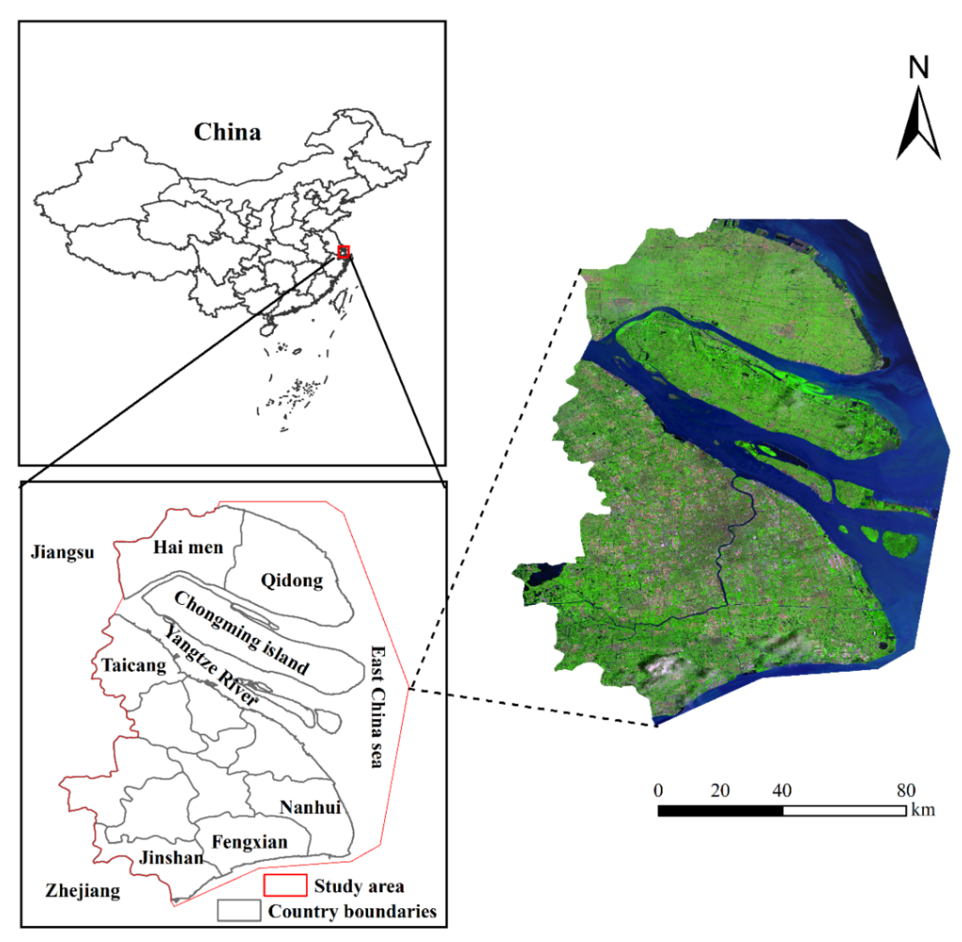
Figure 1. Location of the study area.
Sustainability 12 00659 g001
Figure 2. The designed framework that combines object-based image analysis, hierarchical classification, and updating and backdating approaches for LULC mapping in this study.
Sustainability 12 00659 g002
Figure 3. The class hierarchy for updating/backdating. The initial classification classes are marked in gray, and the misclassified classes are marked in white.
Sustainability 12 00659 g003
Figure 4. Annual time series of LULC maps of the Yangtze River estuary region from 1985 to 2016.
Sustainability 12 00659 g004
Figure 5. Long-term changes in LULC types from 1985 to 2016.
Sustainability 12 00659 g005
Figure 6. Monitoring of gradual changes and sudden changes in Chongming Dongtan wetland from 1985 to 2016 using annual time-series of Landsat data.
Sustainability 12 00659 g006
Table 1. Imagery used for mapping land use and land cover (LULC) and time assignment for updating/backdating.
Year“Spring” “Summer”“Autumn”Image for Tidal Flat MappingTime Assignment for Updating /Backdating
198523/04/198419/08/198620/11/198521/02/1985T−5
198618/05/198719/08/198620/11/198521/02/1985T−4
198718/05/198703/07/198828/12/198718/05/1987T−3
198818/05/198703/07/198830/10/198913/01/1988T−2
198901/12/198911/08/198930/10/198911/08/1989T−1
199026/05/199014/08/199004/12/199014/08/1990T0
199113/04/199218/07/199220/10/199122/02/1991T+1
199231/05/199218/07/199220/10/199118/07/1992T+2
199331/03/199303/06/199320/10/199131/03/1993T−2
199405/05/199412/08/199516/11/199505/05/1994T−1
199508/05/199512/08/199516/11/199516/11/1995T0
199624/04/199618/09/199718/11/199624/04/1996T−4
199711/04/199718/09/199720/10/199711/04/1997T−3
199814/04/199804/08/199808/11/199808/11/1998T−2
199901/04/199924/09/199903/11/199908/11/1998T−1
200027/04/200002/09/200005/11/200002/09/2000T0
200121/03/200103/07/200116/11/200102/09/2000T+1
200208/03/200230/07/200211/11/200211/11/2002T+2
200308/03/200202/08/200329/10/200302/08/2003T−5
200411/05/200519/07/200424/11/200419/07/2004T−4
200511/05/200512/06/200527/11/200512/06/2005T−3
200620/04/200602/08/200627/11/200520/04/2006T−2
200707/04/200728/07/200719/11/200820/04/2006T−1
200811/05/200806/07/200819/11/200811/05/2008T0
200928/04/200919/09/200903/12/201028/04/2009T−4
201025/05/201020/05/201103/12/201027/12/2010T−3
201126/04/201120/05/201106/11/201228/04/2012T−2
201228/04/201229/08/201306/11/201228/04/2012T−1
201325/05/201329/08/201317/11/201329/08/2013T0
201428/05/201429/08/201304/11/201429/08/2013T+1
201512/03/201503/08/201503/12/201612/03/2015T+2
201617/05/201620/07/201603/12/201603/12/2016T+3
Table 2. LULC classification scheme in the Yangtze River estuary.
ClassDescription
ImperviousBuilt-up land, roads, transportation, residential, commercial services, industrial areas and settlements in villages
CroplandAreas cultivated with crops such as rice, beans, and maize
ForestAreas dominated by trees or shrubs, > 30% vegetation cover
GrassLawns and grassland
Inland waterWater bodies located inland
Coastal marshesSaltmarsh and reclaimed marsh that was converted from saltmarsh, > 30% vegetation cover
Barren tidal flatIntertidal mudflat, < 30% vegetation cover
Nearshore water Estuarine water bodies beyond the coastline, shallow seawater
Other barren land Barren land and transactional lands (reclaimed land) that are likely to change or be converted to other uses in the further
Table 3. Methods for updating/backdating for different error types.
Reference Class (T0) Initial Classified Class (Ti)Backdating/Updating to ClassFeatures/MethodReference Values of Features
ImperviousCroplandImperviousEVIave, NDBIaveEVIave < 0.2 & NDBIave > −0.06
ImperviousUnused landImperviousEVIave, NDBIaveNDBIave > 0
CroplandForestCroplandEVIaveEVIave > 0.2
CroplandGrassCroplandEVIaveEVIave > 0.18
CroplandImperviousCroplandEVIave, NDBIaveEVIave > 0.2 & NDBIave < −0.16
CroplandInland waterCroplandEVIaveEVIave > 0.15
ForestCroplandForestVisual interpretation-
ForestGrassForestVisual interpretation-
GrassCroplandGrassVisual interpretation-
GrassForestForestVisual interpretation-
Inland waterCroplandInland waterMNDWIaveMNDWIave > −0.05
Inland waterUnused landInland waterMNDWIaveMNDWIave > 0
Unused landImperviousUnused landVisual interpretation-
Unused landCroplandCroplandVisual interpretation-
Unused landInland waterInland waterVisual interpretation-
Table 4. Land use and land cover sample sizes (n) and sample allocation of each class for validation.
Class/Year198519921998200520112016
Impervious86152204294345405
Cropland10771014974905842767
Forest505050505050
Grass505050505050
Inland water606561666875
Coastal marshes505050505050
Barren tidal flat807372606767
Unused land 505050505050
Total (n)150315041511152515221514