Optimizing the Rail Profile for High-Speed Railways Based on Artificial Neural Network and Genetic Algorithm Coupled Method

Abstract

Though the high-speed railways are seen as a sustainable form of transportation, the fact that the rail wear in high-speed railways negatively affects the running safety and riding comfort, as well as the maintenance of railways, has drawn a wide range of concerns among researchers and scholars. In order to reduce the rail wear and achieve the goal of sustainable transportation, this paper proposes an ingenious optimization program of rail profiles based on the artificial neural network (ANN) and genetic algorithm (GA) coupled method. The candidate solutions of the nonlinear GA programming model are regarded as the inputs of the trained ANN model. Meanwhile, the outputs of the trained ANN model serve as the objective functions of the GA model. The computational results show that the optimized rail profile not only has superior performances in terms of the wheel/rail wear and contact conditions, but also maintains good dynamic performances. Therefore, this study can provide the theoretical and practical basis for the design and the preventive grinding of rails in the high-speed railways. Also, the ANN-GA coupled model can be extended and further employed on the optimization of other rail profiles.

1. Introduction

High-speed railways in China had reached 35,000 km by the end of 2019 (http://society.people.com.cn/GB/n1/2020/0101/c1008-31530914.html). With the rapid growth of the operating mileage and train density, non-uniform rail wear has become one of the critical damages to track infrastructures, and the costs of maintenance and replacements of rails caused by wheel/rail wear are billions of CNY (China Yuan) per year in China [1]. Moreover, the deteriorated running stability and safety as well as the ride comfort of trains will be incurred by the severe rail wear. The root cause of the rail wear is the wheel–rail profile matching because the wheel/rail profiles will directly affect the interaction between them. However, at present, very few existing researches have focused on the optimization of rail profiles aiming at reducing rail wear in high-speed railways. Considering the peculiarities of high-speed railway, such as large volumes of passenger flows and busy lines [2], the time for maintenance is short and the workload is heavy. As a consequence, it is necessary to reduce the rail wear by optimizing rail profiles with a proper method. Besides, the optimized rail profiles, which will eliminate the defects of the rails’ decarburized layer and reduce wheel/rail wear, can achieve the goal of prolonging the rail service life and cutting down the expenses of maintenance.

Traditionally, the trial-and-error method was employed to design the rail/wheel profile, which was mainly based on railway engineers’ experience. Recently, many advanced design methods of rail/wheel profiles have been proposed, benefiting from the rapid development of optimization techniques. Cui et al. [3] proposed a concept of wheel profile design by evaluating the lateral force and the stability of wheelsets, and then the requirements of the wheel profile geometry were investigated through the proposed optimization method. Zeng et al. [4] presented a multi-objective optimization model of pre-grinding profile, in which the objective functions were the nodal accumulated contact stress (NACS) and nodal mean contact stress (NMCS) Kriging models. Wang et al. [5] designed a rail profile for heavy haul railways in terms of the conformance between wheel and rail profiles around contact points for all possible wheel–rail contact situations. Jahed et al. [6] employed a numerical optimization approach to optimize the wheel profile, in which the research target was rolling radii difference (RRD). Persson et al. [7] used a genetic algorithm (GA) optimization method to develop an improved rail profile for Stockholm underground. Ignesti et al. [8] presented two innovative wheel profiles, specifically designed with the aim of improving the wear and stability behavior of the standard ORE S1002 wheel profile. Shevstov et al. [9,10] presented a numerical optimization method for wheel profile design, in which the RRD was employed as an optimization criterion. Wang et al. [11] proposed an improved sequential quadratic programming (SQP) method for optimizing rail profiles to improve vehicle running stability in the switch panel of high-speed railway turnouts.

It can be concluded that plenty of advanced optimization techniques were proposed to design rail/wheel profiles, and it is obvious to see the advantages of these methods. However, due to the complex nonlinear relationship of the interaction between rails and wheels, the formulations of objective functions in numerical optimization methods are difficult to obtain. Moreover, many assumptions are put forward in order to easily obtain these mathematical expressions, whereas the accuracy of optimized results may be degraded. Considering the excellent ability of the artificial neural network (ANN) to solve complex nonlinear problems without the need for specific mathematical expressions [12], this method can get rid of the difficulties of accurately expressing the relationship between design variables and objective functions. Therefore, an ANN model is put forward in this paper. With the rapid development of artificial intelligence, the ANN has been widely adopted in wear research. Singh et al. [13] used a back propagation neural network (BPNN) to predict the flank wear of high-speed steel drill bits for drilling holes on a copper work piece. Kumar and Singh [14] employed ANN to predict wear loss quantities of A390 aluminum alloy. The experimental results were trained in the ANNs program and the predicted results coincided with the experimental results. Shebani and Iwnicki [15] developed nonlinear autoregressive models with exogenous input neural network (NARXNN) for wheel and rail wear prediction.

In this paper, an ANN-GA coupled model is developed for the optimization of rail profiles from the perspective of rail wear. The optimization method developed in this paper is shown in Figure 1. Firstly, the Chinese 60N rail, which has been widely used in China high-speed railways, is optimized by employing the developed model, and points-to-be-optimized of the rail profile are chosen among the major contact area. Then, the new rail profiles satisfying the constraints are input to the multibody dynamics-rail wear (MDRW) model to calculate the rail wear. Afterward, the data of points-to-be-optimized and corresponding objective functions related to rail wear are divided into training sets and testing sets. Later, an ANN model is developed in this paper, in which the coordinates of points-to-be-optimized as input data and corresponding objective functions related to rail wear as output data are employed. The ANN model is trained and tested by the datasets mentioned above. Then, the candidate solutions of the nonlinear constrained GA model are regarded as input data of the trained ANN model, and in the meantime, the output data of the trained ANN model are employed as objective functions of the GA model. The optimized rail profile can be obtained by the ANN-GA coupled model. Finally, the performances of optimized and original rail profiles are compared in the wear developments of the wheel/rail and dynamic behaviors of the track/vehicle.

2. Rail Profile Design

This section presents the mathematical descriptions for the rail profile design.

2.1. Variables Design

The Chinese 60N rails have been widely employed in China high-speed railways. Also, according to a large amount of the onsite observations, it is found that the width of the contact bands is usually 20 to 30 mm at the top of rails [16]. Consequently, the points-to-be-optimized are chosen among the −20 mm to +20 mm region at the top of rails, as shown in Figure 2. This region is divided into n + 1 curve segments. The points at both ends are fixed at y and z coordinates, but the points-to-be-optimized are only fixed at y coordinates. As a result, the changes of these target points in z directions are able to generate different rail profiles by cubic splines. Moreover, the number of points-to-be-optimized not only impacts on the accuracy of the optimized results but also the scale of the optimization procedure. Considering that, 10 points-to-be-optimized are chosen.

2.2. Objective Function

The wear of rails which will change the profiles may have an impact on the running safety and ride comfort. Therefore, it is important to develop an objective function that can accurately describe the wear of the region to be optimized. The objective function developed in this paper is expressed as follows:

$$\min F(Z)=\min {\displaystyle \sum _{m=1}^M{\alpha }_m}\cdot F_m(z_1,z_2,z_3,\dots ,z_n)=\min {\displaystyle \sum _{m=1}^M{\alpha }_m}\cdot \sqrt{{\displaystyle \sum _{i=1}^n{(w_i^m-{\overline{w}}^m)}^2}} ({\displaystyle \sum _{m=1}^M{\alpha }_m}=1)$$

(1)

where m is mth type of vehicle, α_m represents the weight of the mth type of vehicle, in which the influences of the types of vehicles, running speed, and other factors can be considered, and the value of it can be settled based on demand. z₁, z₂, z₃, …, z_n are the z coordinates of the design variables, $w_i^m$ denotes the rail wear of the mth type of vehicle’s ith point-to-be-optimized, and ${\overline{w}}^{\mathrm{m}}$ is the average rail wear of the mth type of vehicle’s all points-to-be-optimized.

The rail wear mentioned in the objective function is evaluated by the means of the MDRW model, and the MDRW model consisting of the multibody dynamics model and the wear model is introduced in the following subsections.

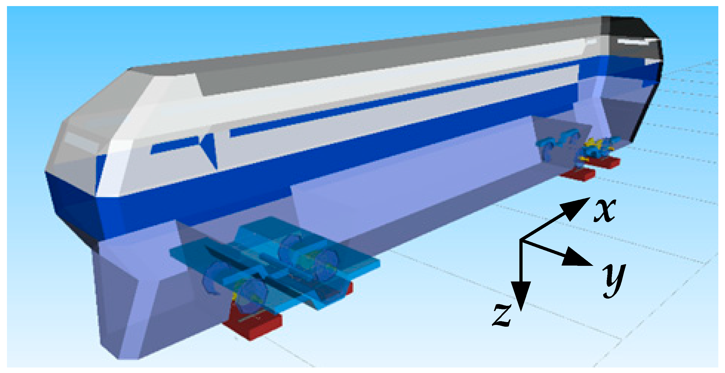
2.2.1. Multibody Dynamics Model

The vehicle model is built with detailed suspensions, as described, which consists of one car body and two bogies, and each bogie is made up of one frame, two wheelsets, and four axel boxes. The whole vehicle model established by SIMPACK is made up of 15 rigid bodies and 50 degrees of freedom in all, as listed in

Table 1. The degrees of freedom of the vehicle model.

Rigid Body Name	Longitudinal	Lateral	Vertical	Roll	Pitch	Yaw
Car body	xc	yc	zc	φc	γc	Φc
Frame	xfi	yfi	zfi	φfi	γfi	Φfi
Axle box	None	None	None	None	γai	None
Wheelset	xwi	ywi	zwi	φwi	γwi	Φwi

. Moreover, the force elements within the primary and secondary suspensions are nonlinear force elements, including spring stiffnesses and dampers. Further parameters of the vehicle model can be found in Xin et al. [17]. In order to simulate actual operational conditions, irregularities of the high-speed railways measured on site are adopted in the model, as shown in Figure 3. Furthermore, the moving track model is applied in this paper, which consists of rails, fasteners, and the track slab, and the detail parameters of the moving track model can be found in Zhai [18], as shown in Figure 4. In this model, dynamic simulations are conducted on a track including tangent and curved sections, and the parameters of the track are listed in

Table 2. The parameters in dynamic simulations.

Parameter	Value	Parameter	Value
Rail cant	1/40	Rail gauge (mm)	1435
Radius of curve (m)	7000	Superelevation (mm)	150
Length of transition curve (m)	670	Length of circular curve (m)	2000
Length of tangent section before curved section (m)	1380	Length of tangent section after curved section (m)	280
Running speed (km/h)	300

. The results of dynamic simulations, such as contact points positions, contact forces, creepages, and so on, are input to the wear model for the calculations of rail wear.

2.2.2. Wear Model

The wear model is established based on Archard’s wear law [19], which has been widely used to calculate the wear caused by the contact friction between objects. The original formula is expressed as follows:

$${\mathrm{V}}_{wear}=k_{wear}\frac{N\cdot s}{H}$$

(2)

where V_wear is the wear volume, k_wear is the wear coefficient, N is the normal contact force, s is the sliding distance, and H is the surface hardness of the softer material.

The FASTSIM algorithm is used to analyze the tangent contact within contact patches, and Hertz’s contact theory is employed to analyze the normal contact. The contact ellipse is discretized first into many rectangle elements, and then the normal stress at the center of a discrete element can be calculated as follows:

$$p_z(x,y)=\frac{3N}{2\pi ab}\sqrt{1-{\left(\frac{x}{a}\right)}^2-{\left(\frac{y}{b}\right)}^2}$$

(3)

where (x, y) denotes the coordinates of the center of a discrete element in the contact patch’s coordinate system, and a and b represent the lengths of the semi-major axis and the semi-minor axis of the elliptical contact patches, respectively. In order to calculate the wear depth in a discrete element, the normal stress at the center of a discrete element is assumed to be the normal stress of the element, and then the wear depth in the element is evaluated as follows:

$$\mathsf{\Delta }{z}_{wear}(x,y)=k_{wear}\frac{p_z\mathsf{\Delta }d}{H}$$

(4)

where Δd is the elastic deformation in time interval Δt and it can be calculated by Equation (5):

$$\mathsf{\Delta }d=\left|S\right|\mathsf{\Delta }t=\sqrt{s_x^2+s_y^2}·\frac{\mathsf{\Delta }x}{V_c}$$

(5)

where S = [s_x s_y]^T is the total slip speed obtained by the FASTSIM algorithm, V_c is the velocity of the center of a discrete element related to the contact patch, and Δx represents the length of a discrete element in the running direction. Substituting Equations (3) and (5) into Equation (4), the wear depth in each discrete element can be obtained as follows:

$$\mathsf{\Delta }{z}_{wear}(x,y)=\frac{3N{k}_{wear}}{2\pi abH}\sqrt{1-{\left(\frac{x}{a}\right)}^2-{\left(\frac{y}{b}\right)}^2}·\sqrt{s_x^2+s_y^2}·\frac{\mathsf{\Delta }x}{V_c}$$

(6)

where the wear coefficient k_wear can only be obtained from a large number of onsite experiments. However, due to the large volumes of passenger flows and busy lines of high-speed railways in China, not enough experiments can be conducted. Therefore, there is no wear coefficient for high-speed railways in China at present. However, many researchers and scholars [20,21,22,23] have used the wear coefficient obtained from the commuter rail system in Stockholm to study the wheel/rail wear, which indicates that this wear coefficient can be suitable for various conditions, including the wheel/rail wear in China high-speed railways. Therefore, the wear coefficient adopted in this paper is depicted by Figure 5 according to the commuter rail system in Stockholm (Jendel [24]).

For each time step of the calculation (2 × 10⁻³ s), the wear of all discrete elements in contact patches along the running direction is summed, and it is regarded as the total wear of the rail profile caused by one rolling circle of a wheel. By summing up the wear of four wheels on the same side, the distributions of rail wear can be obtained when a vehicle passes one time.

2.2.3. Model Verification

The running speed of the vehicle, the radius of the curve, the length of the transition curve, and the super-elevation are: 250 km/h, 6000 m, 180 m, and 70 mm, respectively. In addition, the German high-speed track spectrum is adopted as irregularities. The operating conditions are the same as those in Zhai [18], and the dynamic responses of the multibody dynamics model established in this paper and Zhai [18] are listed in

Table 3. The comparison of dynamic responses.

Evaluation Index	This Paper	Zhai [18]
Vertical wheel-rail force (kN)	132.33	140.89
Lateral wheel-rail force (kN)	19.01	24.38
Derailment coefficient	0.21	0.29

.

It can be seen that the maximum values of the established model are close to those of Zhai [18]. Therefore, it indicates the correctness of the multibody dynamics model established in this paper.

2.3. Constraint Function

To achieve optimization goals that conform to the actual conditions, it is necessary to apply constraints on variables.

Constraint function a: The determination of rail profiles must satisfy the requirement of the convex curve, that is, the slope of adjacent points decreases with the increase of y coordinates. The constraint function is expressed as follows:

$$\frac{z_i-z_{i+1}}{y_i-y_{i+1}}>\frac{z_{i+1}-z_{i+2}}{y_{i+1}-y_{i+2}} (i=1,2,3,\dots ,n-2)$$

(7)

where (y_i, z_i) are the coordinates of the ith point-to-be-optimized in the optimized region of the rail profile.

Constraint function b: Optimizations of rail profiles are carried out based on the original rail profiles, so the optimized profiles should be located below the original rail profiles. Moreover, optimized rail profiles should satisfy the requirement of the maximum grinding depth, which is limited to 2 mm according to the management measures in China. Therefore, the constraint functions are expressed as follows:

$$\{\begin{array}{l}{l}_i\le z_i\le u_i\\ 0\le \mathsf{\Delta }{z}_i\le 2\end{array} (i=1,2,3,\dots ,n)$$

(8)

where l_i and u_i are the lower and upper limits of the ith point-to-be-optimized respectively, and Δz_i is the difference in z coordinate of the ith point-to-be-optimized between the original profile and the new one.

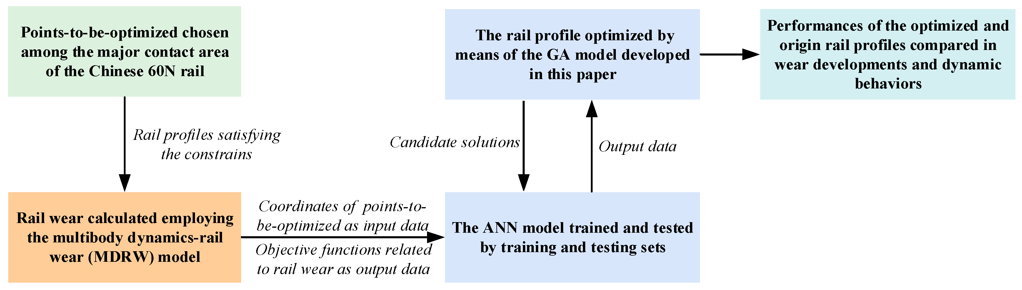
3. Optimization Model

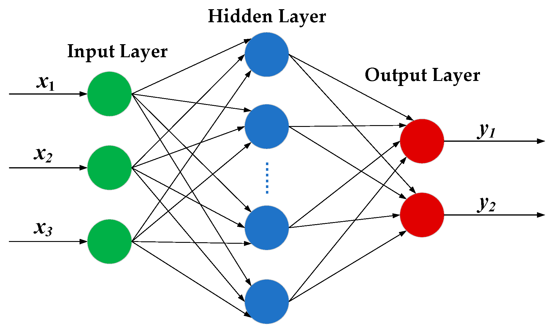
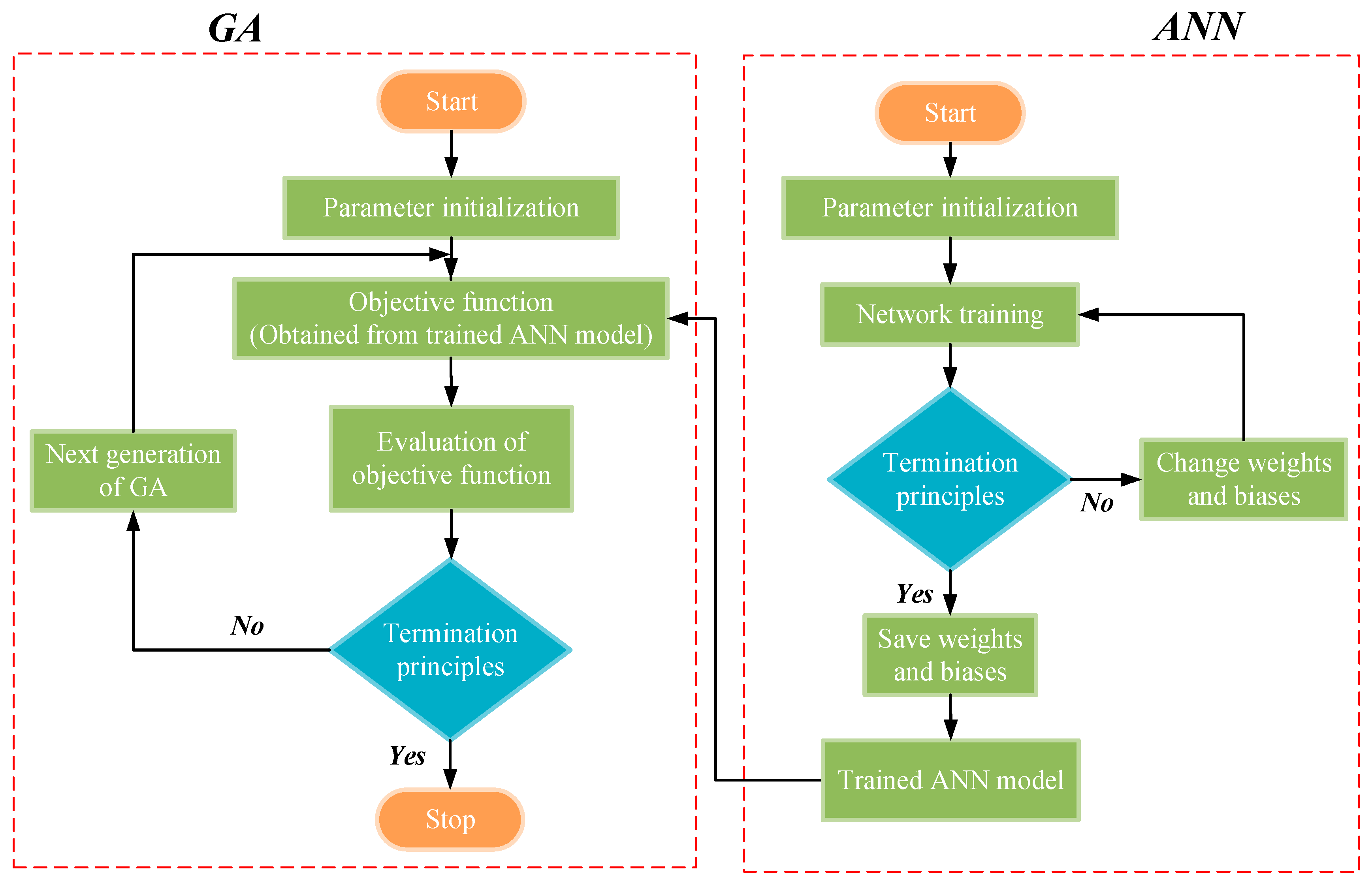
Considering that the objective function of each generation needs to be obtained in the optimization process of the GA model, it is very cumbersome and difficult to calculate the rail wear of each generation and then substitute it into the objective function to obtain the objective function of each generation. Therefore, some sets of the variables and corresponding objective function data are obtained to train the ANN model, and then the cumbersome process mentioned above can be replaced with the trained ANN model. The inputs to this trained ANN model are the candidate solutions of the non-linear constrained GA model, and the outputs of this ANN model are the objective functions of the GA model as well. As a consequence, the functions of predicting the objective functions related to rail wear and optimizing the rail profiles are both significant to achieve the optimization process of rail profiles. Moreover, the ANN-GA coupled method makes the optimization process simple and effective.

3.1. ANN Model

Similar to the biological neural networks that constitute human/animal brains, an ANN is based on a collection of connected units or nodes called artificial neurons, as shown in Figure 6. In an ANN, these nodes are essentially a series of mathematical functions that receive weighted inputs. After processing the inputs, these nodes transfer the outputs to other nodes of the next layer (if any). An ANN is trained to predict the outputs by modifying the weights [25,26,27].

The prediction accuracy of an ANN is usually determined by activation functions, training algorithm, the number of hidden layers and nodes, and arrangement of nodes [28]. Multi-layer perceptron (MLP) is one of the most widely used ANNs for the regression analysis [29]; therefore, MLP is employed in this paper. As for the MLP model developed in this paper, the hyperbolic tangent sigmoid function and the linear function are adopted in the hidden layer and output layer, respectively, and the Levenberg–Marquardt algorithm is employed for training. According to Hornik et al. [30], a three-layer BPNN, which has one hidden layer, can approximate any function at any precision well, given a sufficient number of hidden-layer nodes. Therefore, one hidden layer is applied to the MLP model proposed in this paper, and the number of nodes in the hidden layer is determined by the means of the trial-and-error method based on the training data, as shown in Figure 7. It can be found from Figure 7 that when the number of hidden-layer nodes is 15, the value of mean square error (MSE), which is expressed by Equation (9), becomes minimum. Also, the variation tendency of MSE is rising with the increase of the number of hidden-layer nodes. As a result, the number of hidden-layer nodes is taken as 15 in the MLP model developed in this paper.

$$MSE=\frac{1}{Q}{\displaystyle \sum _{q=1}^Q{(T_q-y_q)}^2}$$

(9)

where Q is the number of the dataset, T_q is the qth target value of the dataset, and y_q is the qth predicted value of the dataset.

In this paper, the prediction steps of the MLP model are as follows [25]:

Step 1: The input of a node in the hidden layer is summed up with the weighted inputs and a constant bias, which is formulated by Equation (10):

$$n_r={\displaystyle \sum _{p=1}^P{w}_{pr}{x}_p+b_r} (r=1,2,3,\dots ,R)$$

(10)

where p and r are the pth node of the input layer and rth node of the hidden layer respectively, P and R are the number of nodes in the input layer and the hidden layer, x_p is the input to the MLP model, w_pr and b_r are the weight and constant bias of the hidden layer respectively, and n_r is the input to the rth node of the hidden layer.

Step 2: After applying the activation function to all the nodes of the hidden layer, the output of a node in the hidden layer is expressed as follows:

$$H_r=g(n_r)=g({\displaystyle \sum _{p=1}^P{w}_{pr}{x}_p+b_r})$$

(11)

where g(x) is the activation function, which is the hyperbolic tangent sigmoid function, and H_r is the output of the rth node in the hidden layer.

Step 3: The activation function of the output layer is linear. Therefore, the output of a node in the output layer is summed up with weighted outputs from the hidden layer and a constant bias, which is expressed by Equation (12):

$$y_k={\displaystyle \sum _{r=1}^R{w}_{rk}{H}_r+b_k} (k=1,2,3,\dots ,K)$$

(12)

where k is the kth node of the output layer, K is the number of nodes in the output layer, w_rk and b_k are the weight and constant bias of the output layer respectively, and y_k is the output of the kth node in the output layer.

Step 4: The updates of weights in the hidden layer and the output layer are expressed by Equations (13) and (14), respectively:

$$w_{pr}=w_{pr}+\eta H_r(1-H_r)x_p{\displaystyle \sum _{k=1}^K{w}_{rk}(T_k-y_k)}$$

(13)

$$w_{rk}=w_{rk}+\eta H_r(T_k-y_k)$$

(14)

where η is the learning rate.

Step 5: The updates of biases in the hidden layer and the output layer are formulated by Equations (15) and (16), respectively:

$$b_r=b_r+\eta H_r(1-H_r){\displaystyle \sum _{k=1}^K{w}_{rk}(T_k-y_k)}$$

(15)

$$b_k=b_k+\eta (T_k-y_k)$$

(16)

Following the above steps, the MLP model can be mathematically expressed as follows:

$$y_k={\displaystyle \sum _{r=1}^R{w}_{rk}g({\displaystyle \sum _{p=1}^P{w}_{pr}{x}_p+b_r})+b_k (k=1,2,3,\dots ,K)}$$

(17)

3.2. GA Model

GA is a heuristic search that is inspired by Charles Darwin’s theory of natural evolution. Compared with tradition techniques, the advantages of GA are as follows: (1) it can search the solution globally and not easily fall into local minima and (2) it can effectively avoid differential operation on variables [31].

GA begins with a population that represents a potential set of solutions to a problem, while a population consists of a certain number of individuals encoded by genes. Each individual is actually an entity with characteristic chromosomes, which determine the external representation of shapes of individuals. Therefore, mappings from the phenotype to the genotype, that is, encoding work, need to be implemented at the beginning. Since the gene encoding is complex, it must usually need to be simplified, such as the binary encoding. After the initial generation of the population, according to the survival-of-the-fittest principle, the evolution of each generation produces better and better approximate solutions. In each generation, it is based on the fitness of the individual to make selections. The new population is generated utilizing genetic operators, which consist of combination, crossover, and mutation. This process will cause the descendant population to be more adaptable to the environment than the previous population, and the best individual in the last generation population is decoded, which can be used as the approximate optimal solution to a problem [26].

Generally speaking, the penalty function is employed to solve optimization problems with nonlinear constraints [32,33]. The penalty makes sure that any search space which violates nonlinear constraints will be abandoned. The nonlinear constraints are usually handled by creating an augmented Lagrangian form called subproblem for the original problem [34], which is formulated by Equation (18):

$$\min \theta (x,\lambda ,l,\rho )=F(x)-{\displaystyle \sum _{i=1}^d{\lambda }_i{l}_i\log (l_i-C_i(x))}+{\displaystyle \sum _{\mathrm{j}=1}^e{\lambda }_{j}Ce{q}_j(x)}+\frac{\rho }{2}{\displaystyle \sum _{j=1}^{e}Ce{q}_j{(x)}^2}$$

(18)

where F(x) is the objective function, d and e are the number of inequality and equality nonlinear constraints respectively, C(x) and Ceq(x) are, separately, inequality and equality nonlinear constraints, λ is the non-negative Lagrange multiplier, l is the slack variable, ρ is the penalty parameter, and the augmented Lagrangian subproblem is minimized in the nonlinear constrained GA.

In each iteration, the Lagrange multipliers are fixed. Therefore, the subproblems do not reach minima until the termination principles are achieved. What calls for special attention is that since the subproblem extracts the nonlinear constraints from the primal problem, only linear constraints and bounds need to be satisfied. The procedure for the optimization of rail profiles employing the ANN-GA coupled optimization method is shown in Figure 8.

4. Results and Discussion

In the optimization process, all parameters are consistent with the actual operational conditions, which are listed in Table 2, and the detailed geometric parameters of the Chinese 60N rail profile are illustrated in Figure 9. Moreover, three types of vehicle models mainly operating in high-speed railways are employed in the optimization process, which are equipped with S1002CN, XP55, and LMA wheel profiles, respectively. The three types of wheel profiles are shown in Figure 10. The influences of different wheel profiles are considered by weighting in their objective functions, as expressed in Equation (1), in which the weight values of three types of vehicles are all set as 1/3.

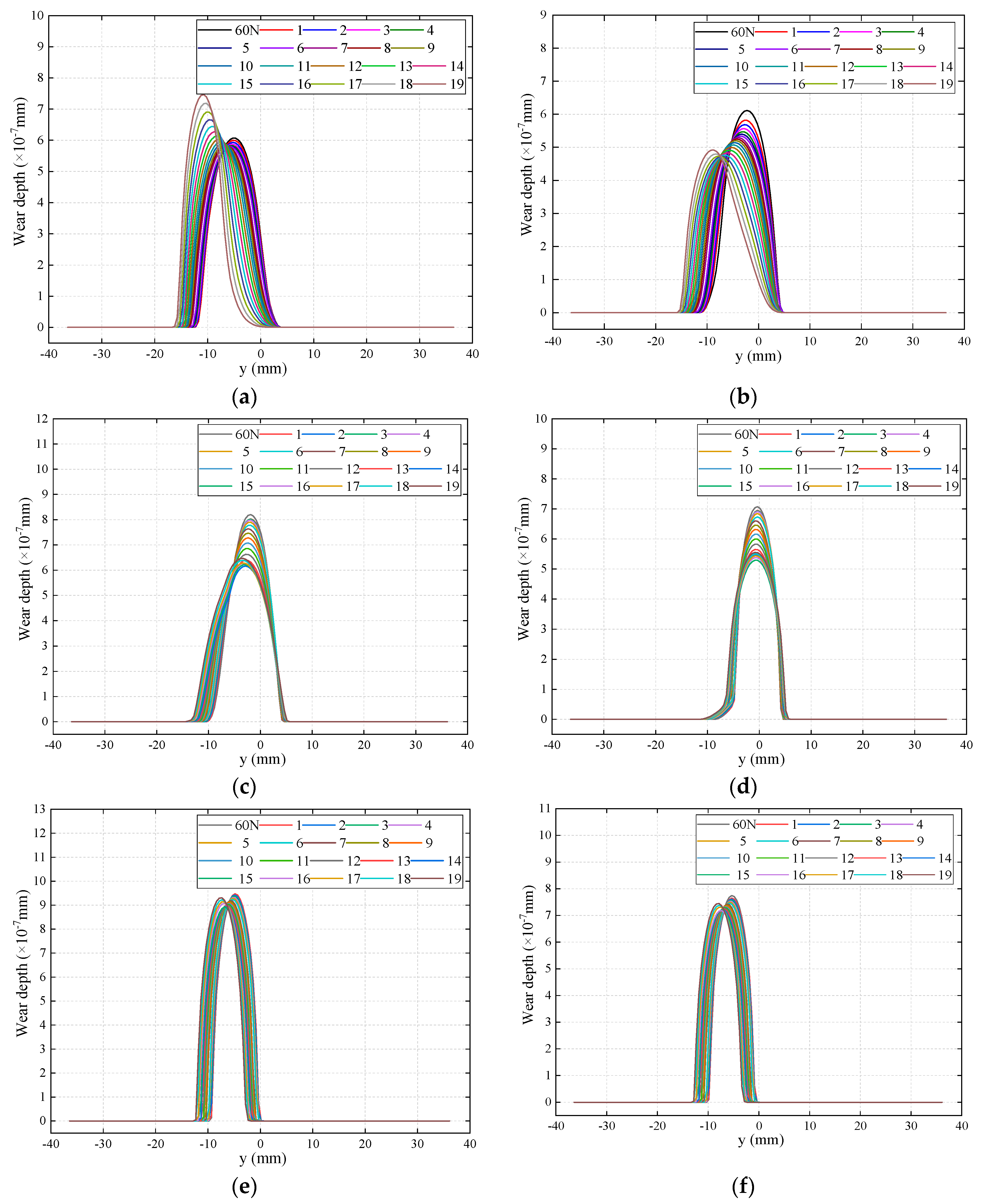
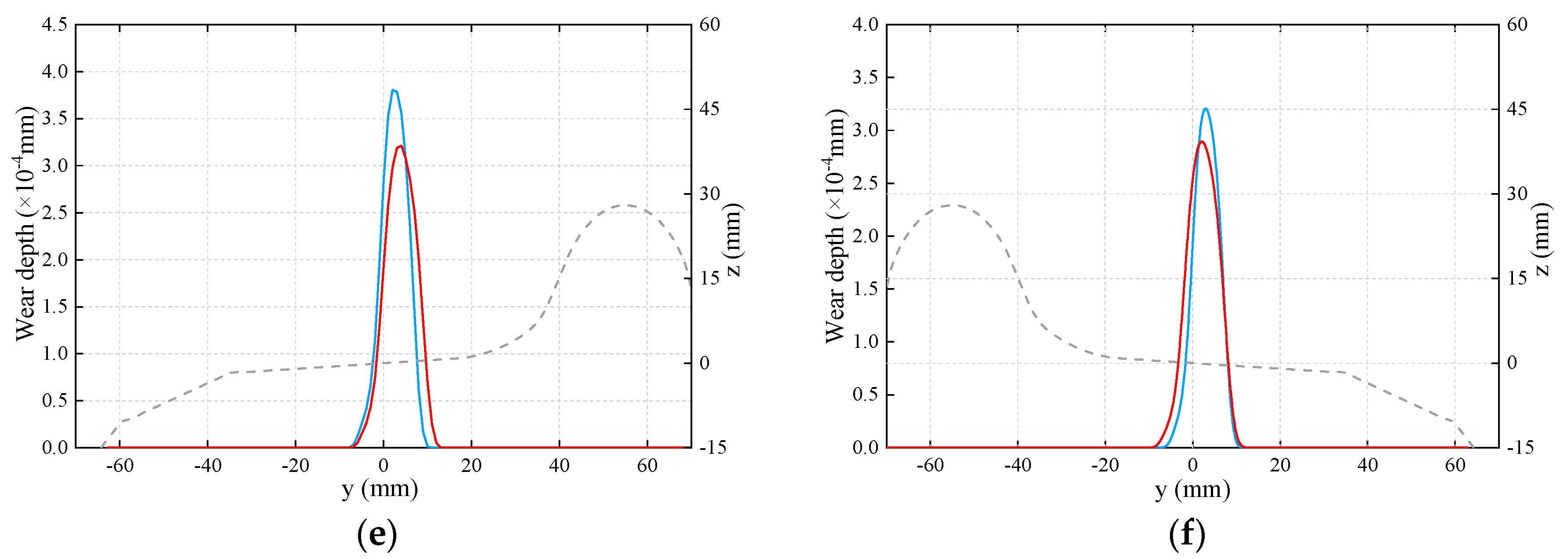
4.1. Simulation Results of MDRW Model

According to the constraint functions, 20 sets of satisfactory rail profiles were generated, as shown in Figure 11. The profiles were input to the MDRW model to calculate rail wear and objective functions, and the results are described in Figure 12 and Figure 13, respectively.

It can be observed from Figure 12 that the main wear regions of different rail profiles are concentrated at the rail heads, which is from −20 mm to 10 mm. Also, due to the deficient super-elevation in the curved section, the wear of the left rails as the outer rails is more severe than that of the right rails. However, the deficient super-elevation is only 1.7 mm, so the rail shoulders of the left rails will not appear worn. With the growth of the distances from new profiles’ rail heads to the original ones, the wear of both side rails performs as decreasing previously and increasing later. Therefore, the optimal solution should appear in the range of 20 sets of rail profiles.

Figure 13 indicates the objective functions of the left rail, right rail, and the sum of them, and it can be observed that the trends of objective functions are in good agreement with the wear of 20 sets of rail profiles. As a consequence, the objective functions developed in this paper can effectively demonstrate the mapping relationship between design variables and rail wear. Considering that the optimized profile should be suitable for left and right rails, the sum of left and right rail’s objective functions is regarded as the final objective function in this paper.

4.2. Prediction Accuracy of the ANN Model

In this paper, the input data are the z coordinates of points-to-be-optimized, and the output data are the corresponding values of the objective function. Moreover, 20 sets of data including 220 data points are adopted to train and test the ANN model, as listed in

Table 4. The datasets adopted in the ANN model.

Datasets	Input Data (×–1 mm)										Output Data (×10−7 mm)
1	1.292	0.633	0.257	0.088	0.010	0.010	0.088	0.257	0.633	1.292	13.8580
2	1.302	0.657	0.290	0.125	0.048	0.048	0.125	0.290	0.657	1.302	13.6690
3	1.312	0.682	0.323	0.162	0.087	0.087	0.162	0.323	0.682	1.312	13.6080
4	1.321	0.707	0.356	0.198	0.125	0.125	0.198	0.356	0.707	1.321	13.4005
5	1.331	0.731	0.389	0.235	0.163	0.163	0.235	0.389	0.731	1.331	13.2630
6	1.341	0.756	0.422	0.271	0.202	0.202	0.271	0.422	0.756	1.341	13.0758
7	1.351	0.780	0.455	0.308	0.240	0.240	0.308	0.455	0.780	1.351	13.0643
8	1.361	0.805	0.488	0.345	0.279	0.279	0.345	0.488	0.805	1.361	13.0418
9	1.371	0.829	0.520	0.381	0.317	0.317	0.381	0.520	0.829	1.371	12.9944
10	1.381	0.854	0.553	0.418	0.355	0.355	0.418	0.553	0.854	1.381	12.9913
11	1.391	0.878	0.586	0.455	0.394	0.394	0.455	0.586	0.878	1.391	12.9652
12	1.401	0.903	0.619	0.491	0.432	0.432	0.491	0.619	0.903	1.401	12.9441
13	1.411	0.928	0.652	0.528	0.471	0.471	0.528	0.652	0.928	1.411	12.9136
14	1.421	0.952	0.685	0.565	0.509	0.509	0.565	0.685	0.952	1.421	12.8299
15	1.431	0.977	0.718	0.601	0.547	0.547	0.601	0.718	0.977	1.431	12.7234
16	1.440	1.001	0.751	0.638	0.586	0.586	0.638	0.751	1.001	1.440	12.6435
17	1.450	1.026	0.784	0.675	0.624	0.624	0.675	0.784	1.026	1.450	12.6669
18	1.460	1.050	0.817	0.711	0.663	0.663	0.711	0.817	1.050	1.460	12.6900
19	1.470	1.075	0.849	0.748	0.701	0.701	0.748	0.849	1.075	1.470	12.9405
20	1.480	1.099	0.882	0.785	0.739	0.739	0.785	0.882	1.099	1.480	13.3525

. Among these data, 80 percent of the data are taken randomly as the training set and the remaining data are treated as the testing set, respectively. The relative errors of prediction results with target values based on testing data are listed in

Table 5. The relative errors based on testing data.

Number of Rail Profiles	Prediction Result (×10−7 mm)	Target Value (×10−7 mm)	Relative Error ξ (%)
16	12.6435	10.5575	0.9141
3	13.6080	9.7627	−2.2523
15	12.7234	10.3132	−0.5516

, and the mathematical expression of relative error is expressed by Equation (19).

$$\xi =\frac{x_p-x_t}{x_t}\times 100\%$$

(19)

where x_p is the prediction result and x_t is the target value.

It can be observed from Table 5 that the relative errors are all controlled below 3%. Moreover, the relative errors show that the trained MLP model can effectively illustrate the mapping relationship between inputs and outputs. As a result, the outputs of the MLP model can be employed as the objective functions of the GA model.

4.3. Optimizaiton Results of the ANN-GA Coupled Model

4.3.1. Optimization Process

The initial population is generated randomly in the range of constraint function b, and the optimization process is conducted based on the initial population. The candidate solutions of the GA model are input to the trained ANN model, and the outputs from the trained ANN model are regarded as the objective functions of the GA model. The two-directional iterative process of the ANN-GA coupled model is conducted until the minimum value of the objective function is obtained. The variation trend of the fitness with the increase of the generation is illustrated in Figure 14. It can be seen that the maximum fitness and the average fitness all remain constant after 100 generations. The optimization result can be obtained after 100 iterations, and the optimized rail profile is generated by cubic splines, as shown in Figure 15. In addition, the objective functions obtained by the ANN-GA model and the MDRW model are 11.936 × 10⁻⁷ mm and 11.785 × 10⁻⁷ mm respectively, and the relative error is only 1.28%. Therefore, the optimization result of the ANN-GA model is in perfect agreement with that of the MDRW model.

4.3.2. Wear Performances

The wear of both side rails and leading wheelsets are separately calculated by the MDRW model, in which the parameters of the track are listed in Table 2. The wheel wear of the leading wheelsets is depicted in Figure 16. It can be concluded that, due to the use of the optimized rail profile, the left and right wheels’ wear depth becomes smaller than those of the original rail profile. In addition, the maximum wear depth appears to be on the left wheel of XP55. After applying the optimized rail profile to three types of vehicles, the wear regions of both side wheels basically become larger, but they are still in the center regions of the wheel profiles.

With regards to the wear of both side rails, the results are presented in Figure 17. After applying the optimized profile to three types of vehicles, the wear depths of both side rails are smaller than those of the original profile. Also, because of the deficient super-elevation in the curved section, the wear depth of left rails as the outer rails is bigger than that of right rails, whether employing the optimized rail profile or not. The maximum wear depth also appears to be on the left rail of XP55. For both side rails, the wear areas are extended after employing the optimized profile. Therefore, the wear distributions of rail heads are more uniform, and the occurrence of concentrated wear is decreased.

4.3.3. Dynamic Performances

To compare and analyze the dynamic performances when employing the optimized and original rail profiles, the vehicle-track coupled dynamic model is established, as mentioned in Section 2.2.1. The parameters of the track are listed in Table 2.

Considering the running safety and stability, it is worth noting that the evaluation indexes include the vertical/lateral wheel-rail force, derailment coefficient, wheel load reduction ratio, and area of contact patch. The peak values of these evaluation indexes when employing the original profile and the optimized profile are illustrated in Figure 18. As for the area of contact patch, the average values are also listed. The statistical histograms of the vertical/lateral wheel–rail force, derailment coefficient, and the wheel load reduction ratio are illustrated in Figure 19, and the time history curves of contact patch area are shown in Figure 20. Moreover, the derailment coefficient and the wheel load reduction ratio can be calculated by Equations (20) and (21).

$$\frac{F_L}{F_V}=\frac{\tan \alpha -\mu }{1+\mu \cdot \tan \alpha }$$

(20)

where F_L is the lateral wheel–rail force, F_V denotes the vertical wheel–rail force, α is the angle of wheel flange, and μ denotes the wheel–rail friction coefficient.

$$\frac{\mathsf{\Delta }W}{\overline{W}}=\frac{W_1-W_2}{W_1+W_2}$$

(21)

where ΔW is the quantity of the wheel load reduction, $\overline{W}$ is the average static wheel load, and W₁ and W₂ denote the two sides of wheel loads, respectively.

From Figure 18 and Figure 19, it can be found that very small differences, when comparing the original profile with the optimized profile under three conditions, exist in the vertical/lateral wheel–rail force, derailment coefficient, and wheel load reduction ratio. Moreover, the statistical distributions of these indexes mentioned above all show tends of normal distributions, approximately. Except for the lateral wheel–rail force of S1002CN, the peak values of the other three evaluation indexes all declined. As for the lateral wheel-rail force of S1002CN, the peak values of the optimized profile only increased by 3.13%. However, the peak values of the vertical wheel–rail force, derailment coefficient, and wheel load reduction ratio were much smaller than the limiting values in corresponding regulations [35].

Unlike the other evaluation indexes, it can be observed from Figure 18e,f, and Figure 20 that the differences of the contact patch area are obvious when comparing the optimized profile with the original profile under three conditions. After using the optimized profile, the contact patch area becomes larger and the maximum increment can reach up to 46.87%, which appears in the peak value of LMA. As a result, employing the optimized profile can improve the contact conditions between rails and wheels.

To sum up, the differences are very small on the whole, though sometimes the dynamic responses of the optimized profile are bigger than those of the original profile, except for the area of contact patch. Moreover, the peak values of both profiles are much smaller than limiting values. As a result, the optimized profile not only achieves the optimization goal but also maintains good dynamic performances.

4.3.4. Effectiveness Evaluation

To evaluate the optimization effectiveness of the ANN-GA coupled method proposed in this paper, the increment of the area of contact and the decrease of the maximum contact pressure are compared with that obtained by the method developed in Cui et al. [36]. The comparisons of the two evaluation indexes are listed in

Table 6. The comparisons of evaluation indexes.

Evaluation Index	S1002CN	LMA	XP55	Cui et al. [36]
Increment of the area of contact	29.59%	33.00%	25.08%	16.11%
Decrease of the maximum contact pressure	28.06%	33.65%	26.21%	23.50%

. It can be observed that the method proposed in this paper performs better than that developed in Cui et al. [36].

5. Conclusions

In this paper, an ANN-GA coupled optimization method was developed to optimize the rail profile. The ANN model was developed by feeding forward back-propagation neural networks with the MLP structure. The input data were the coordinates of points-to-be-optimized and the output data were the objective functions related to the rail wear. The prediction model was able to predict the objective functions with accuracy above 97%. Therefore, it can indicate that the prediction model is accurate and efficient.

The trained ANN model coupled with the GA model was developed in this paper, which has multiple nonlinear constraints. The candidate solutions of the GA model were input to the trained ANN model, and the outputs from the trained ANN model were regarded as the objective functions of the GA model. The two-directional iterative process of the ANN-GA coupled model were conducted until the minimum value of the objective function was obtained.

The related error of the optimized rail profile’s objective function predicted by the ANN-GA coupled model was only 1.28%, compared with that calculated by the MDRW model. Therefore, the validity of the optimized rail profile can be proved. Then, the optimized profile and the original profile were systematically compared in aspects of the wheel/rail wear and dynamic performances, and the MDRW model developed in this paper was used to conduct the comparative study. It can be found from computational results that the wear depth of the optimized rail profile was smaller, and the wear distributions were more uniform. The wear depth of wheels of the leading wheelset became smaller after adopting the optimized rail profile as well. Furthermore, the differences of the vertical/lateral wheel–rail force, derailment coefficient, and wheel load reduction ratio were very small. Moreover, they were much smaller than the limiting values. As for the contact patch area, the differences in the contact patch area were obvious. After using the optimized rail profile, the contact patch area became larger, and the increment can reach to 46.87%. Therefore, employing the optimized profile can improve the contact conditions between rails and wheels.

Conclusions can be drawn that the optimized rail profile not only has superior performances in terms of the wheel/rail wear and contact conditions but also maintains good dynamic performances. The present work in this paper aimed to propose the ingenious ANN-GA coupled method theoretically and then the optimized rail profile was compared and analyzed by simulating. Finally, this study can provide the theoretical and practical basis for the design and the preventive grinding of rails used in the high-speed railways. Moreover, the ANN-GA coupled model can also be used for the optimization of other rail profiles.

References

1. Liu, J.; Wang, W.; Liu, Q. Matching Characteristics between Four Kinds of Wheel Steels and U71Mn Hot-Rolled Rail. J. Southwest Jiaotong Univ. 2015, 50, 1130–1136. [Google Scholar]
2. Ollivier, G.; Bullock, R.; Jin, Y.; Zhou, N. High-speed railways in China: A look at traffic. China Transp. Top. 2014, 11, 1–12. [Google Scholar]
3. Cui, D.; Wang, R.; Allen, P.; An, B.; Li, L.; Wen, Z. Multi-objective optimization of electric multiple unit wheel profile from wheel flange wear viewpoint. Struct. Multidiscip. Optim. 2019, 59, 279–289. [Google Scholar] [CrossRef] [Green Version]
4. Zeng, W.; Qiu, W.; Ren, T.; Sun, W.; Yang, Y. Multi-Objective Optimization of Rail Pre-Grinding Profile in Straight Line for High Speed Railway. J. Shanghai Jiaotong Univ. (Science) 2018, 23, 527–537. [Google Scholar] [CrossRef]
5. Wang, P.; Gao, L.; Xin, T.; Cai, X.; Xiao, H. Study on the numerical optimization of rail profiles for heavy haul railways. Proc. Inst. Mech. Eng. Part F J. Rail Rapid Transit 2017, 231, 649–665. [Google Scholar] [CrossRef]
6. Jahed, H.; Farshi, B.; Eshraghi, M.A.; Nasr, A. A numerical optimization technique for design of wheel profiles. Wear 2008, 264, 1–10. [Google Scholar] [CrossRef]
7. Persson, I.; Nilsson, R.; Bik, U.; Lundgren, M.; Iwnicki, S. Use of a genetic algorithm to improve the rail profile on Stockholm underground. Veh. Syst. Dyn. 2010, 48, 89–104. [Google Scholar] [CrossRef]
8. Ignesti, M.; Innocenti, A.; Marini, L.; Meli, E.; Rindi, A.; Toni, P. Wheel profile optimization on railway vehicles from the wear viewpoint. Int. J. Non-Linear Mech. 2013, 53, 41–54. [Google Scholar] [CrossRef] [Green Version]
9. Shevtsov, I.; Markine, V.; Esveld, C. Optimization of Railway Wheel Profile Using MARS Method. In Proceedings of the 43rd AIAA/ASME/ASCE/AHS/ASC Structures, Structural Dynamics, and Materials Conference, Denver, CO, USA, 22–25 April 2002; p. 1320. [Google Scholar]
10. Shevtsov, I.Y.; Markine, V.L.; Esveld, C. One procedure for optimal design of wheel profile. In Proceedings of the IQPC Conference on Achieving Best Practice in Wheel/Rail Interface Management, Amsterdam, The Netherlands, 31 January–1 February 2002. [Google Scholar]
11. Wang, P.; Ma, X.; Wang, J.; Xu, J.; Chen, R. Optimization of rail profiles to improve vehicle running stability in switch panel of high-speed railway turnouts. Math. Probl. Eng. 2017, 2017, 2856030. [Google Scholar] [CrossRef]
12. Kramer, M.A. Nonlinear principal component analysis using autoassociative neural networks. Aiche. J. 1991, 37, 233–243. [Google Scholar] [CrossRef]
13. Singh, A.K.; Panda, S.S.; Chakraborty, D.; Pal, S.K. Predicting drill wear using an artificial neural network. Int. J. Adv. Manuf. Technol. 2006, 28, 456–462. [Google Scholar] [CrossRef]
14. Kumar, A.; Singh, D. Artificial neural network-based wear loss prediction for a390 aluminium alloy. J. Theor. Appl. Inf. Technol. 2008, 4, 961–964. [Google Scholar]
15. Shebani, A.; Iwnicki, S. Prediction of wheel and rail wear under different contact conditions using artificial neural networks. Wear 2018, 406–407, 173–184. [Google Scholar] [CrossRef] [Green Version]
16. Juanjuan, R.; Huawei, Z.; Ming, O. Influence of rail grinding on wheel-rail contact relationship for high-speed railway. J. Huazhong Univ. Sci. Technol. (Natural Science Edition) 2016, 44, 95–100. [Google Scholar]
17. Xin, T.; Wang, P.; Ding, Y. Effect of Long-Wavelength Track Irregularities on Vehicle Dynamic Responses. Shock Vib. 2019, 2019, 4178065. [Google Scholar] [CrossRef]
18. Zhai, W. Vehicle-Track Coupled Dynamics, 4th ed.; China Science Publishing & Media Ltd.: Beijing, China, 2014. [Google Scholar]
19. Archard, J. Contact and rubbing of flat surfaces. J. Appl. Phys. 1953, 24, 981–988. [Google Scholar] [CrossRef]
20. Xu, J.; Wang, P.; Wang, J.; An, B.; Chen, R. Numerical analysis of the effect of track parameters on the wear of turnout rails in high-speed railways. Proc. Inst. Mech. Eng. Part F J. Rail Rapid Transit 2018, 232, 709–721. [Google Scholar] [CrossRef]
21. Luo, R.; Shi, H.; Teng, W.; Song, C. Prediction of wheel profile wear and vehicle dynamics evolution considering stochastic parameters for high-speed train. Wear 2017, 392, 126–138. [Google Scholar] [CrossRef]
22. Bevan, A.; Molyneux-Berry, P.; Eickhoff, B.; Burstow, M. Development and validation of a wheel wear and rolling contact fatigue damage model. Wear 2013, 307, 100–111. [Google Scholar] [CrossRef] [Green Version]
23. Iwnicki, S. The effect of profiles on wheel and rail damage. Inte. J. Veh. Struct. Syst. 2009, 1, 99–104. [Google Scholar] [CrossRef]
24. Jendel, T. Prediction of wheel profile wear—Comparisons with field measurements. Wear 2002, 253, 89–99. [Google Scholar] [CrossRef]
25. Sebaaly, H.; Varma, S.; Maina, J.W. Optimizing asphalt mix design process using artificial neural network and genetic algorithm. Constr. Build. Mater. 2018, 168, 660–670. [Google Scholar] [CrossRef] [Green Version]
26. Pappu, S.M.J.; Gummadi, S.N. Artificial neural network and regression coupled genetic algorithm to optimize parameters for enhanced xylitol production by Debaryomyces nepalensis in bioreactor. Biochem. Eng. J. 2017, 120, 136–145. [Google Scholar] [CrossRef]
27. Khudhair, A. Neural Network Analysis for Sliding Wear of 13% Cr Steel Coatings by Electric Arc Spraying. Diyal. J. Eng. Sci. 2010, first, 157–169. [Google Scholar]
28. Schmidhuber, J. Deep learning in neural networks: An overview. Neural Netw. 2015, 61, 85–117. [Google Scholar] [CrossRef] [Green Version]
29. Kavzoglu, T.; Mather, P.M. The use of backpropagating artificial neural networks in land cover classification. Int. J. Remote Sens. 2003, 24, 4907–4938. [Google Scholar] [CrossRef]
30. Hornik, K.; Stinchcombe, M.; White, H. Multilayer feedforward networks are universal approximators. Neural Netw. 1989, 2, 359–366. [Google Scholar] [CrossRef]
31. Deb, K. Optimization for Engineering Design: Algorithms and Examples; PHI Learning Pvt. Ltd.: New Delhi, India, 2012. [Google Scholar]
32. Conn, A.R.; Gould, N.I.; Toint, P. A globally convergent augmented Lagrangian algorithm for optimization with general constraints and simple bounds. Siam. J. Numer. Anal. 1991, 28, 545–572. [Google Scholar] [CrossRef] [Green Version]
33. Deb, K. An efficient constraint handling method for genetic algorithms. Comput. Methods Appl. Mech. Eng. 2000, 186, 311–338. [Google Scholar] [CrossRef]
34. Conn, A.; Gould, N.; Toint, P. A globally convergent Lagrangian barrier algorithm for optimization with general inequality constraints and simple bounds. Math. Comput. Am. Math. Soc. 1997, 66, 261–288. [Google Scholar] [CrossRef]
35. China, S.A. Technical regulations for dynamic acceptance for high-speed railways construction. In TB 10761-2013; Standards Press of China: Beijing, China, 2013. [Google Scholar]
36. Cui, D.; Li, L.; Jin, X. Study on Rail Goal Profile by Grinding. Eng. Mech. 2011, 28, 178–184. [Google Scholar]
Figure 1. The framework of the optimization method in this paper.
Sustainability 12 00658 g001
Figure 2. The illustration of design variables.
Sustainability 12 00658 g002
Figure 3. (a) The lateral irregularities and (b) vertical irregularities.
Sustainability 12 00658 g003
Figure 4. The multibody dynamics model.
Sustainability 12 00658 g004
Figure 5. The Archard wear coefficient.
Sustainability 12 00658 g005
Figure 6. The structure of an artificial neural network (ANN). (xi and yi are the input and output, respectively).
Sustainability 12 00658 g006
Figure 7. The relationship between the number of hidden-layer nodes and mean square error (MSE).
Sustainability 12 00658 g007
Figure 8. The ANN-GA (genetic algorithm) coupled optimization method.
Sustainability 12 00658 g008
Figure 9. The geometric parameters of the Chinese 60N rail profile.
Sustainability 12 00658 g009
Figure 10. The three types of wheel profiles.
Sustainability 12 00658 g010
Figure 11. The satisfactory rail profiles.
Sustainability 12 00658 g011
Figure 12. The wear depth of (a) left rails of S1002CN, (b) right rails of S1002CN, (c) left rails of LMA, (d) right rails of LMA, (e) left rails of XP55, and (f) right rails of XP55.
Sustainability 12 00658 g012
Figure 13. The illustration of objective functions.
Sustainability 12 00658 g013
Figure 14. The variation of fitness.
Sustainability 12 00658 g014
Figure 15. The original and optimized profiles.
Sustainability 12 00658 g015
Figure 16. The wear depth of (a) left wheels of S1002CN, (b) right wheels of S1002CN, (c) left wheels of LMA, (d) right wheels of LMA, (e) left wheels of XP55, and (f) right wheels of XP55. (The red, blue and grey lines refer to optimized profiles, the original profiles, and wheel profiles, respectively).
Sustainability 12 00658 g016aSustainability 12 00658 g016b
Figure 17. The wear depth of (a) left rails of S1002CN, (b) right rails of S1002CN, (c) left rails of LMA, (d) right rails of LMA, (e) left rails of XP55, and (f) right rails of XP55. (The red, blue and purple lines refer to optimized profiles, the original profiles, and rail profiles, respectively).
Sustainability 12 00658 g017aSustainability 12 00658 g017b
Figure 18. The evaluation indexes of dynamic performances (the red and blue bars refer to optimized profiles and the original profiles, respectively.) Note: (ae) are peak values, and (f) is the average value. The values on the top of the purple dotted lines are the limiting values.
Sustainability 12 00658 g018
Figure 19. The statistical histograms of (af) vertical/lateral wheel–rail force, (gi) derailment coefficient, and (jl) wheel load reduction ratio of S1002CN, LMA, and XP55, respectively. (The red and blue bars refer to optimized profiles and the original profiles, respectively).
Sustainability 12 00658 g019aSustainability 12 00658 g019b
Figure 20. The time history curves of contact patch area of (a) S1002CN, (b) LMA, and (c) XP55 (the red and blue lines refer to optimized profiles and the original profiles, respectively).
Sustainability 12 00658 g020