Article

Efficient Structural Design of a Prefab Concrete Connection by Using Artificial Neural Networks

by
Jorge Navarro-Rubio
1,
Paloma Pineda
2,* and
Roberto Navarro-Rubio
1
1
NR Proyectos—Engineering and Architectural Consulting, Calle Constantino nº 49 1º I, 04700 Almería, Spain
2
Department of Building Structures and Geotechnical Engineering, Universidad de Sevilla, Avda, Reina Mercedes, 2, 41012 Seville, Spain
*
Author to whom correspondence should be addressed.
Sustainability 2020, 12(19), 8226; https://doi.org/10.3390/su12198226
Submission received: 7 September 2020 / Revised: 24 September 2020 / Accepted: 4 October 2020 / Published: 6 October 2020

Abstract

:
In the built environment, one of the main concerns during the design stage is the selection of adequate structural materials and elements. A rational and sensible design of both materials and elements results not only in economic benefits and computing time reduction, but also in minimizing the environmental impact. Nowadays, Artificial Neural Networks (ANNs) are showing their potential as design tools. In this research, ANNs are used in order to foster the implementation of efficient tools to be used during the early stages of structural design. The proposed networks are applied to a dry precast concrete connection, which has been modelled by means of the Finite Element Method (FEM). The parameters are: strength of concrete and screws, diameter of screws, plate thickness, and the posttensioning load. The ANN input data are the parameters and nodal stresses obtained from the FEM models. A multilayer perceptron combined with a backpropagation algorithm is used in the ANN architecture, and a hyperbolic tangent function is applied as an activation function. Comparing the obtained predicted stresses to those of the FEM analyses, the difference is less than 9.16%. Those results validate their use as an efficient structural design tool. The main advantage of the proposed ANNs is that they can be easily and effectively adapted to different connection parameters. In addition, their use could be applied both in precast or cast in situ concrete connection design.

1. Introduction

In different engineering fields, the use of Artificial Neural Networks (ANNs) is gaining a noticeable position in the material design and selection stages. These computational models are powerful tools that allow for not only reducing computing times, but also designing adequate shapes and reducing the amount of raw materials used. As a consequence, ANNs have the potential to significantly reduce both economic cost and environmental impact.
Artificial Neural Networks (ANNs) are biologically inspired computational models that are based on the interconnection mechanisms of the human brain’s neurons. These mathematical models are able to solve complex multivariable linear or nonlinear problems and to obtain relationships between different patterns. ANNs have been traditionally applied to different fields, such as financial analysis, image processing (e.g., target recognition and image completion), medical test diagnosis, robot control, and speech recognition. In addition to performing complex computations, they allow for recognizing patterns that can be applied in the learning computation process. ANNs are especially appropriate if the problem has a difficult or non-defined solving procedure [1].
The main advantage of using neural networks is their ability to learn from experience, generalizing from previous situations to new cases and differentiating essential information from that which is irrelevant. ANNs are able to represent and learn both linear and non-linear relationships directly from the data [2].
Since 1986, the use of ANNs was spread due to the feasibility of developing an error back-propagation training algorithm, which was based on a gradient-descent optimization technique [3]. In addition, ANNs have gained a relevant position in solving industrial design problems. It is worth mentioning that the identification of the optimum design within an industrial process is not always possible due the size of the problem and lack of knowledge, as the design stage is essential [2]. However, ANNs are able to perform constraint checks, requiring less computing time to provide adequate results.
Focusing on civil engineering, it is worth mentioning that although ANNs were developed in the seventies [4], their applications in civil and structural engineering date from 1989 [5]. In 2001, Hojjat published a review on Neural Networks in Civil Engineering [5], where the use of ANN from 1989 to 2001 in civil, structural, and building engineering fields was analyzed. Gupta et al [6] analyzed the feasibility of using ANNs in structural analysis and building design from 1990 to 2011. Amezquita-Sanchez et al. [7] published a review paper analyzing the ANNs’ applications in civil infrastructures. That research focused on structural system identification, structural health monitoring, structural vibration control, structural design and optimization, prediction applications, construction engineering, and geotechnical engineering.
In civil engineering, ANNs have been successfully used in automation and optimization [2,5,8], in material formulation [9], and in system identification and monitoring [10,11]. In structural analysis and design, the following applications could be highlighted [2,6,12]: structural analysis of systems with large degrees of freedom, size optimization of structural members, joint location, shape optimization of structural types (e.g., truss geometry), topology optimization (based on deletion of ineffective structural members), and maximum stress identification and location. Focusing on the application to specific structural problems, Intelligent Finite Element Analysis (IFEA), which combines the Finite Element Method (FEM) together with an ANN, has been used for simulating or predicting constitutive models [13,14,15]. Waszczyszyn and Ziemianski [16] applied a hybrid ANN to analyze elastoplastic beams together with the Finite Difference and Finite Element methods. Neural Networks have been also applied in structural analysis pattern recognition [17,18]. Regarding prediction applications of ANNs, Lee [19] and De-Cheng et al. [20] analyzed their use for predicting the concrete strength; Yan Cao et al. (2020) analyzed their application in the behavior of beam-to-column connections; Van Dao et al. [21] applied these computational models in the compressive strength prediction of concrete mixed with geopolymer; and Abambres et al. [22] predicted the fatigue strength of concrete. Stoffel et al. [23] proposed an ANN to predict deformations in non-linear metal plates, while Kamgar et al. [24] designed a feed-forward back-propagation neural network (FFBPNN) to be used to propose a new formulation for predicting the compressive strength of fiber-reinforced polymer (FRP)-confined concrete cylinders, and Komleh and Maghsoudi [25] applied an Adaptative Neuro-Fuzzy Inference System (ANFIS) and multiple regression analysis in the prediction of the curvature ductility factor of FRP-strengthened reinforced high-strength concrete beams. Focusing on the use of metaheuristic optimization algorithms to optimize structures, the works by Kaleh et al. [26] and by Kaleh and Dadras [27] are remarkable. Focusing on economic issues, Kamgar et al. [8] proposed a fuzzy inference system to evaluate the building design codes from an economic point of view.
It is worth noting that the use of ANNs in precast concrete elements or connections is an open research field. In fact, neither the prediction of complex nonlinear structural stresses and deformations nor their use in the design stage has been widely analyzed.
The main objective of this research is threefold:
  • To contribute to the optimal design of precast structural components by using ANNs;
  • To minimize the computation time in structural analyses by means of ANNs;
  • To contribute to the implementation of ANNs within the building sector.

2. Materials and Methods

In order to accomplish the aforementioned objectives, this work focuses on the structural design of a specific dry beam–column connection, which has been recently proposed and analyzed by Navarro-Rubio et al. [28]. Four ANNs are designed to predict the structural response of the connection, aiming at designing the materials in an effective way. Each ANN is trained by using numerical data that are obtained from Finite Element analyses (FEM). These analyses are performed with Ansys FEM software [29]. The input data include: (i) material parameters, (ii) relations between adjacent stresses in nodes, and (iii) deformations. All the FEM model parameters are implicitly considered in the ANN input during the learning process. Four Multilayer Perceptrons (MLPs) are proposed to predict the behavior of the elements using a Hyperbolic Tangent Function (HTF) as the activation function.
Due to the stresses’ variability in the precast concrete connection (e.g., nodal stresses are positives and negatives in the same element, in the beam or plate) the HTF function is the most adequate. This function provides a faster convergence and lower error than those of the sigmoidal one. After analyzing the results, the proposed ANNs are validated to be used as a design tool, aiming at reducing computation time, and making easier the structural design stage. The main advantage of the designed ANNs is the easy and effective adaptation to different connection parameters, as well as the feasibility of being used both in precast or cast in situ concrete connections. In general, the numerical software solves one model for each parameter configuration; it is a time-consuming process if many different parameter combinations are required. Actually, in common practice, a considerable number of element connections are expected, and defining the appropriate design for each connection would demand significant computational times. The main reason for developing an ANN is that once it is properly trained, it can be used for solving the design problem for any set of input parameters in a highly efficient manner and with lower computational times (if compared to common numerical procedures).
In the following subsections, the analyzed case study (including the main characteristics of the FEM model) is described. The discrete optimization method that has been used is also presented.

2.1. Description of the Case Study

In order to study both the feasibility and the potential of using ANNs for the design of structural materials and elements, this research focuses on a single case study, the analysis of a dry precast concrete connection that has been recently designed and analyzed by Navarro-Rubio et al. [28].
The connection is designed as follows: Precast concrete beams are connected to a precast concrete column with bolted steel plates (Figure 1 and Figure 2); non-contact tubes inside the column are added for the screw yielding (Figure 1e). A post-tensioned tendon is located in the middle of the beam (Figure 1a and Figure 2).
The connection elements are fabricated in the workshop and connected on-site. In the workshop, after the formwork is built, the steel elements and rebars are located in the final position inside the connection. The final elements are composed of precast concrete beams or columns, with steel plates or tubes for screws or tendons inside them to achieve a faster on-site construction. After removing the formwork, small plates are welded at the bottom of the column’s steel device. The on-site fabrication steps are the following: (i) To place the beams over small plates, the use of cranes is minimized and the on-site construction times are reduced. (ii) Once the beam is placed in the final position, the screws are fastened to connect precast elements. (iii) Finally, the tendon is put inside the strand, and the elements are posttensioned.
Focusing on the advantage of this connection, two main features can be highlighted: the faster on-site construction stage and the feasibility of achieving a monolithic behavior without cast-in-place concrete. In addition, due to the configuration of the elements, it provides better resistance under horizontal loading. An in-depth discussion on the details of the connection design and its advantages is presented in Navarro-Rubio et al. (2019).
The connection structural response is analyzed by means of numerical simulations. A three- dimensional Finite Element Model (FEM) is developed by using the commercial software Ansys [29]. The concrete elements are modelled by means of eight node solid elements (Solid 65), while linear Link180 elements are used to model rebars inside the concrete. These elements are commonly used in structural analyses (e.g., [30]). Solid steel elements, such as plates and tendons, have been modelled with the element Solid 185. To model the contact between elements (concrete–steel in the beam–column interface), the Target170 and Conta173 elements are used. Those elements can simulate pressure under contact, as well as free volume when there is no contact. The elements also consider friction and cohesion. The mesh comprises 37,631 elements (Figure 1b).
Focusing on the materials, a nonlinear behavior is assumed for concrete and for contact areas. Table 1 provides the material control parameters according to the Spanish Concrete Code EHE-08 [31], where the ultimate strength is Fu = Fck + 8 and Young’s modulus is E = 8500 F u 3 .
The Drucker–Prager (DP) perfectly plastic criterion [32] and the Willam–Warncke (WW) failure surface [33] are the theories that are applied to define the behavior of the concrete. As is well known, both theories yield accurate results on solid 3D models. Three-dimensional cracking is permitted in tension and crushing in compression. In a first stage, the material is isotropic, until either the tensile or the compressive strength is exceeded. As the yield surface does not change with progressive yielding, there is no hardening rule, and the material behaves as elastic—perfectly plastic. The values of cohesion, equal to 6.5 MPa, and friction angle, equal to 35°, have been selected to obtain a good match with uniaxial strength in tension and compression. The dilatancy angle, ψ, is equal to 35°. Two shear transfer coefficients for open and closed cracks, βt equal to 0.85 and βc equal to 0.15, are also included. With regard to the steel elements, elastoplastic models are applied for screws, plates, tendons, and rebars.
Regarding the boundary conditions, the base of the column is completely constrained, and both external sides of the beams are partially constrained, allowing only vertical displacement (but neither horizontal nor nodal rotation are allowed), acting as a symmetry axis.
Nonlinear elastic analyses (under incremental loading) are performed. The loading has been gradually applied on the top face of the beams. The loading steps range from 0 to 0.20 MPa, with a step load of 0.02 MPa. A compression load in the beams is also applied by means of the posttensioned tendon (PT-Load). No other load has been applied in the structural elements. The iteration method is that of Newton–Raphson. The controls, force, and displacement tolerances are activated [30] with a limit of 0.05. The calculation finishes when an element joint reaches its strength limit.
As the main focus of the analysis is the material design, different FEM models are built, varying these parameters: (i) concrete strength, (ii) screw diameters, (iii) plate thickness, (iv) PT-Load, and (v) screw strength. The parameter variation is defined in the following section. The results of each step and sub-step are recorded and used as input for the ANNs.

2.2. Efficient Design

In structural analyses, one of the most relevant objectives within design procedures is minimizing the weight of the used materials [2]. It is worth noting that in order to obtain the best and minimal solution that optimizes a structural element or part (e.g., joint or connection), different material and parameter combinations should be compared. Focusing on FEM analyses, the most common and conventional numerical methods require both high pre-processing and computing times.
The applied design and state variables and the objective function are:
(1) Design variables:
-
DT: Diameter of the screw: 12, 16, 20, 22, and 24 mm;
-
EC: Thickness of the beam plate: 15, 20, 25, 30, 35, and 40 mm;
-
PT: Posttensioning load applied: 0, 50, 100, 150, and 200 kN;
-
Concrete strength: 25, 30, 35, and 40 MPa;
-
Screw steel strength: 4.6, 5.6, 6.8, 8.8, and 10.9, where A.B represents the yield (A × B × 10 MPa) and ultimate strength (B × 100 MPa), respectively.
(2) State variables: The main focuses are the stress field distribution and the deflection in the external face of the beam, where the maximum deflection is expected. The vertical surface load increases in each step, while the material strength in the connection keeps under the stress limits.
(3) Objective function: This is the maximum material nodal stress in the connection according to the design variables, as indicated in point number 1.
By using the proposed ANNs, the results of the different combinations are immediately obtained, and it is easier and faster to compare the different structural design configurations.

3. Results and Discussion

The main result of this research is the proposal of an ANN-based procedure to be used in the early design stages of structural materials and elements. In order to guarantee that the designed ANNs are reliable tools, a validation of the network is also required. In the following subsection, the ANN input and the design, selection, and validation procedure are described and explained in detail.

3.1. The FEM Model as ANN Input

As indicated previously, some of the parameter combinations are used in the ANN learning process. If all the combinations were used, the network does not learn; in fact, it only would provide the given data. In ANN design, the learning stage is carried out with a representative sample, and the validation is performed by using data that have not been applied in the learning stage. Once the validation is done, the network will be ready to use.
For the input learning process, the FEM model, as described in Section 2 (description of the case study), has been implemented. The parametric calculations have been carried out by using different values of the variables (Section 2). 
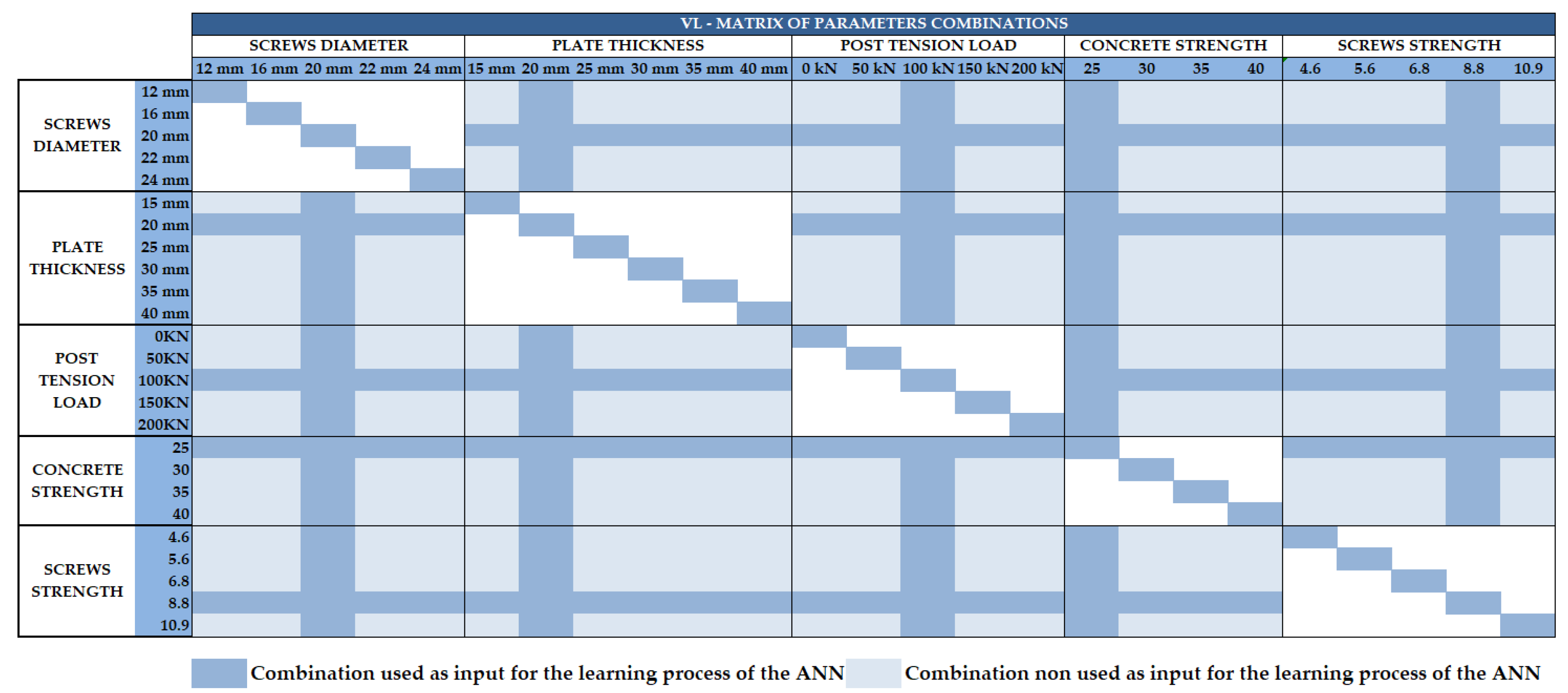
Figure 3 summarizes the parameter combinations and those used in the learning process.
A main concern is to perform a proper selection of the learning process data. For this reason, in this research, the selected sample is representative of all the possible variables, but it is taken into account that most of the parameters (plate thickness, screw diameter and strength, and concrete strength) are not continuous, as they are normalized and standardized discrete industrial values; for instance, screw diameters are 12, 16, 20 mm, etc., but no decimal values are used. The only continuous value could be the post-tensioning load. However, following the actual practice in construction works, common discrete values are also selected for the PT-Load. The number of variables includes the design variables defined in Section 2.2 and provided in Figure 3: (i) six for the plate thickness (15, 20, 25, 30, 35, and 40 mm), (ii) five for the screw diameter (12, 16, 20, 22, and 24 mm), (iii) five for the PT-Load (0, 50, 100, 150, and 200 kN), (iv) four for the concrete strength (25, 30, 35, and 40 MPa), and (v) five for the screw resistance (4.6, 5.6, 6.8, 8.8, and 10.9). Once a variable set has been chosen and fixed, one of them within the set is varied along its range. For instance, keeping the rest of variables fixed (screw diameter, PT-Load, concrete strength, and screw resistance with a fixed value), results will be obtained by varying the sheet metal thickness from 12, 16, 20, 22, and 24 mm, using the results as input for the learning step. That process is repeated with the other variables. For each variable value variation, an FEM model has been built and the numerical data are obtained step by step. This procedure provides a reliable input (2 million units of data), as the ANNs can learn the relationship between stresses in different elements when a parameter is modified, but also the relationships when other parameters are selected.
For each FEM model, an increasing value of the load has been applied over the beam surface. The vertical deformation and nodal stress values have been recorded step by step for each node. All the steps (including the intermediate ones) from the initial and the final stage have been analyzed and saved to be used as input for the learning process. The recorded data have relevant implicit information, as the relationships between stresses and deformations in adjacent nodes are considered in the FEM analysis.
In the combinations that have been used as input, the parameters are recorded in each sub-step of the FEM numerical model, as shown in Table 2. In each combination, the followed structure is the same for all the files in order to allow for an adequate reading and operation for the ANNs. The columns include the step and node number for an easy identification in the numerical model, as well as the material stresses, where σ x and σ y are the concrete stress in the X and Y directions, Vxy and Vxz are the concrete shear stress along the XY and XZ planes, respectively, and σ v m is the Von Misses stress in the steel elements.

3.2. Implementation of the ANNs: Design and Selection of the ANN Models

In this research, four different ANNs have been designed, one per each element: beams, plates, post-tensioning tendon (PT), and screws. The same ANN that has been modelled for the beam could be used to predict column stresses. It is worth mentioning that the column nodes have not been studied because the stresses in the column nodes are lower than those of beams, and no relevant results would be provided.
In the ANN design, a key factor is to obtain a network that is as simple as possible and that does not include non-relevant data. It is worth highlighting that all the information that is provided in FEM model calculations would be high enough to make the network unfeasible.
In this work, as the FEM model implicitly takes into account the strain–stress relation, it is possible to eliminate or neglect the node position, as well as the relation among nodes. The main goal is to predict when a network element is going to collapse. Thus, the network can be dimensioned. Once each element is analyzed for both materials (concrete and steel), the main interest is locating the most loaded node step by step, and comparing it with its limit value. In this way, the network learns the stress increase that is produced by the elements, and that depends on the applied load. Thus, a network for each different element allows for predicting the stress field. Additionally, the designed network learns how a parameter variation influences the stress path (e.g., changing the concrete or screw strengths). Therefore, the network can be applied to any parametric change (e.g., an increase in the structural element dimensions). Moreover, it does not depend on the number of nodes of the numerical model. In the case of not having made the simplification, the number and name of each node should be kept. In this way, a main concern is to be clear on the required data and how to locate them.
The initial stage of the ANN design consists of defining the network architecture. The most common neural networks include an input layer, a hidden layer, and an output layer, as this is enough to solve most problems [17]. In this research, all the ANNs have the same basic structure: a multilayer perceptron developed in C# by using Visual Studio community 2019 [34]. A simple backpropagation algorithm is implemented [
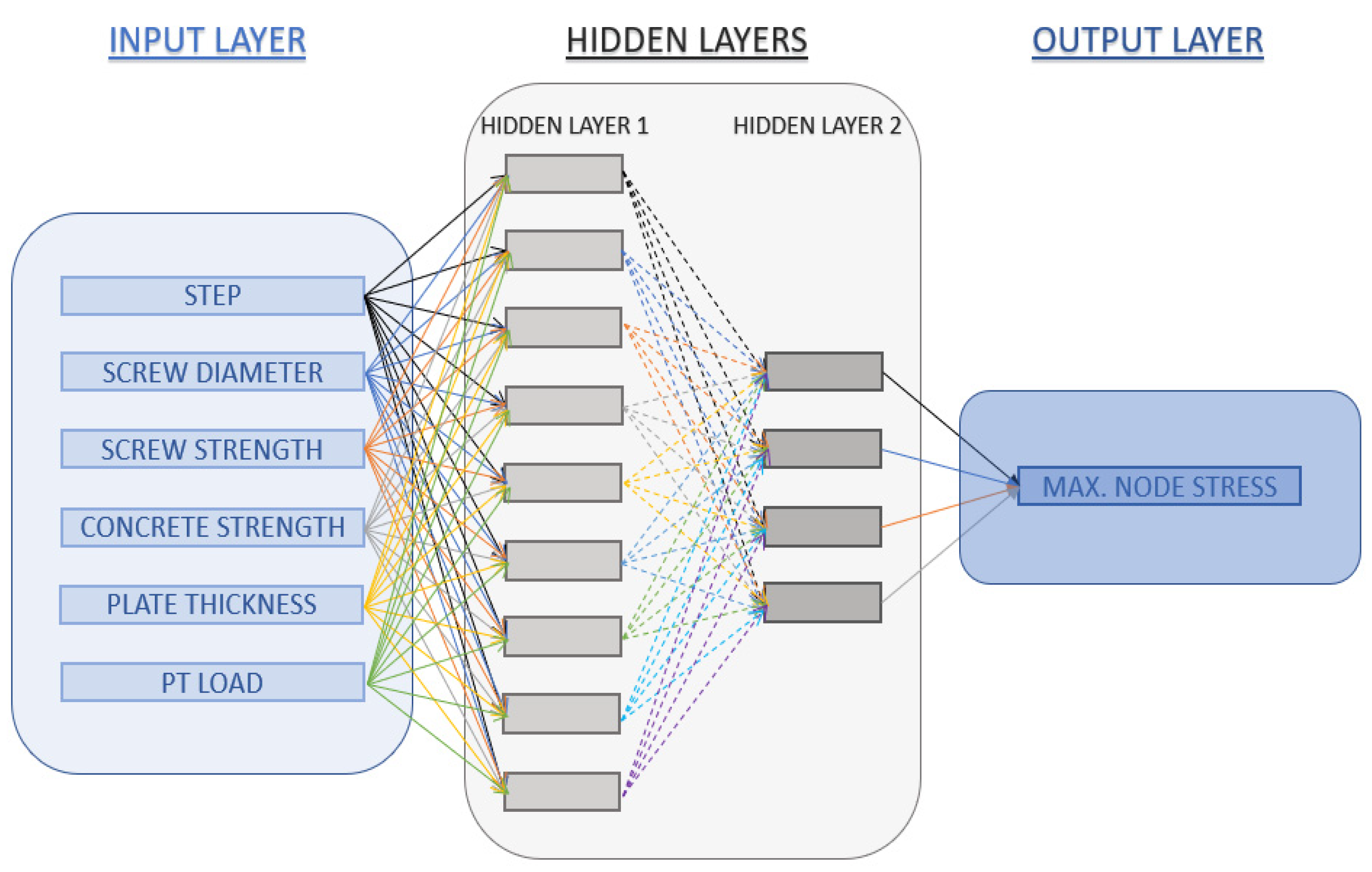
3]. The input layer has six neurons that are the input variables: steps, screw diameter, concrete strength, screw strength, PT-Load, and plate thickness (Figure 3). Regarding the hidden layers, it is worth noting that, in general, one hidden layer is sufficient. However, when the number of neurons in a single layer increases, the predictive efficiency does not increase, and for complex problems, two hidden layers could be required [10,17]. After a trial-and-error stage with one hidden layer and with a neuron number increase, the networks do not converge. For that reason, two hidden layers are required to obtain a faster and better convergence. The number of neurons in the hidden layer depends on the complexity of the ANN, including the number of inputs and outputs or input variable continuity [35]. A minimum number of neurons is required to minimize the output error and to reduce the learning process, but the stability of the network must be guaranteed. The two hidden layers have different neurons depending on the complexity of the calculation and on the dispersion of the input data. The output layer has only one neuron, which is the maximum prediction stress in any element node. Figure 4 depicts the ANN configuration scheme.
In the definition of the ANN topology, a trial-and-error process is required at different stages ([13,17,35,36,37,38]): (i) in the definition of neurons in the hidden layers, (ii) in the testing and learning process, and (iii) in the selection of the random weights. Those trial-and-error procedures make it possible to establish a suitable and stable network. Trial and error may be extended to building several networks, stopping and testing them at different stages of learning, and initializing the network with different random weights. Each network must be tested and analyzed, and the most appropriate network must be chosen in each project. In this research, the followed process required trial-and-error iterations on each network to obtain both good convergence and stability. The numbers of neurons in the hidden layers were gradually increased to reach convergence, and the structure of each ANN is the minimum required to reach that objective. The final configuration and parameters of the designed ANNs are summarized in Table 3.
Due to the field variability of the nodal stress in plates and beams (tensions and compressions are located simultaneously in the element, as well as the sign variation along steps), the ANNs require extra hidden layers to guarantee good convergence.
For a better understanding of the ANN configuration, a flowchart of the ANN algorithm is provided in Figure 5.
One of the main advantages of implementing the use of ANNs within the structural material design stage is the significant decrease in the required computing time if compared to conventional FEM analyses (e.g., those exclusively performed via FEM). Indeed, once the ANN has learned, the estimation is immediately provided for any new configuration. In this study, the time consumed in the learning process was 16 hours for each ANN, using approximately 1.8 million iterations.
The proposed ANN predicts the stiffness matrix solved in the FEM model, providing the maximum expected nodal stress for each element: plates, screws, beams, or tendons. It is worth noting that solving that matrix is one of the most time-consuming steps in FEM analyses. Moreover, the computing time increases exponentially in nonlinear analyses. The data prediction is immediately provided according to the applied input and for any surface loading value applied on the upper face of the beam. In addition, the ANN can solve the nonlinear behavior (in terms of both material and geometry) of the designed connection.
Each step from the FEM model has a direct relationship with the load applied, so an implicit relation between the applied load and the element stresses could be easily obtained (step = load).

3.3. ANN Validation

In the ANN validation, 1.8 million entries have been used. Those entries are distributed in 40 files by randomly varying the parameters. Ten additional numerical calculations have been performed, comparing the elements of the FEM results to the ANN prediction step by step. The parameters that have been applied in the validation are summarized in Table 4. In the selection procedure, a random variation of the parameters has been applied. After that procedure, the FEM model is updated, and the results are compared with those predicted by the ANN.
The maximum and average errors in the learning process are assessed by comparing the actual stress value with the curve of adjustment that the ANN provides. Table 5 summarizes the average nodal stress error in all the steps and sub-steps. The maximum difference, in percentage, between the actual and the predicted stresses is also provided in every node for all the steps and sub-steps. The average error value would be monotonically reduced with the same input in case more iterations were done in the learning process. However, there is a point where its reduction after many iterations is negligible, that is, it becomes asymptotic. If more entries were used, a new learning process would be necessary, and the final error is expected to be lower than the one obtained.
As observed, a maximum error of 7.36% is detected in plates, while the average error is 2.19%. That indicates deviations in some nodes that are located in areas of concentrated stresses (Figure 6), or in steps that are close to the material strength limit. Similar results are detected in screws, beams, and posttensioned tendons.
Four different ANNs have been developed to predict the element results: beam, plate, tendons, and screws. For each FEM model, four comparisons have been made (Figure 7), one for each ANN. In the comparisons, maximum nodal stresses in each element (beam, plate, PT, or screws) per step are provided and compared (in red) with the maximum nodal stress of each step from the FEM numerical analysis (in blue). For concrete, the maximum stress is compared to the maximum principal stress ( σ x σ y ). In the steel elements, the Von Misses stress criterion is used. The load values range from 0 to the maximum obtained in the corresponding FEM analysis. The maximum and average errors are provided.
Regarding FEM values, in Table 6 and Table 7, step-by-step comparisons for each element are depicted. Only the final steps are included.
When the applied loads are increased and the concrete is close to the strength limit, maximum deviations between the predicted stresses and the FEM solutions are obtained. Under 0.08 MPa, the difference is lower than 3%. The maximum stress in concrete when 0.08 MPa is applied is 19.69 MPa. Due to the applications of partial safety factors, as required by Codes [31,39], the maximum concrete stress that is expected in real structures is close to 50% of the strength limit. Thus, the provided stress field is satisfactory enough, accomplishing the Code requirements, and corroborating that the ANN is an efficient design tool.
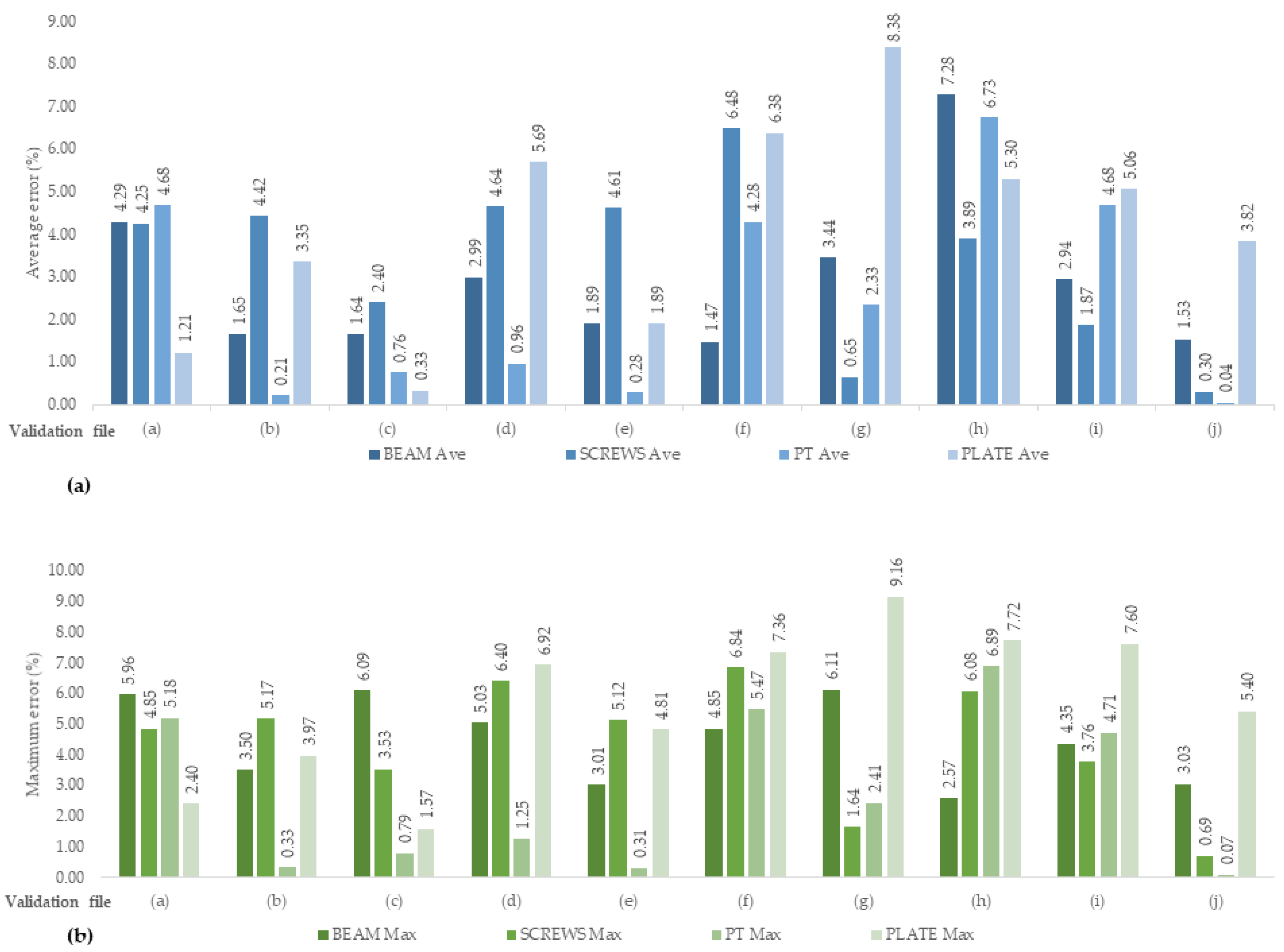
In the validation process, six different parameter combinations from the FEM analysis have been used. The obtained average and maximum errors in each element are summarized in Figure 8.
As observed, a maximum error of 9.16% is obtained in the worst scenario. The maximum errors are obtained in the final steps of each calculation due to the stress concentrations or to the first cracking in concrete. As this situation is an anomaly in the increasing stress curve, the ANN has difficulties in learning and predicting those values. Taking into account that in the most common structural design methods, safety factors are applied, the obtained stress field is around 50% of the strength limit. As observed in Table 6 and Table 7 and Figure 7, the maximum errors appear at the end of the comparison, when concrete is close to the strength limit. It should be noted that for the PT, the maximum error is low, 0.79%. As the average error is lower than 8.38% in all the validation cases, it can be stated that the designed networks are reliable tools for stress prediction and design. The differences between the predicted and the FEM model values in the tensioned parts (i.e., screws or PT tendon) remain stable. More differences are detected in beams (1.47%–6.11%) and plates (0.33%–8.38%), although stresses remain within acceptable ranges.
It is worth noting that the designed ANNs share some features with other research works. Thus, the procedure developed by Ashour et al. [14] is similar to that used in this work, where different ANNs were implemented by varying some parameters and using a back-propagation algorithm with a trial-an-d-error process to determine the number of hidden layers and neurons. In the work by Ashour et al. [14], the network used fewer neurons in one hidden layer. In this research, due to both the variability of the nodal stress field and the number of input data, an extra hidden layer was required. In addition, the number of neurons needs to be increased to reach convergence. In the same research line, Lorenzi et al. [40], after using a back-propagating ANN, highlighted the feasibility of using ANNs to predict concrete compressive strength based on a pull-out test on concrete. Those authors applied different ANNs with three hidden layers and a variable number of neurons in each layer, with a maximum of 80 neurons. In this work, two hidden layers were required, with a maximum of 25 neurons in the beam. That is due to the great number of nodes and to the stress variability in both value and sign when the load increases. Almeida Junior [15] also obtained satisfactory predictive results on the load capacity of adhesive anchors, proposing an ANN with two hidden layers with three and two neurons, and the training process time was 12 seconds. In this research, due to the number of inputs, the number of neurons in the hidden layers, and the number of hidden layers, approximately 16 hours were needed to train the worst scenario. The similar conclusions on time reduction that the ANN provides when compared to common numerical analyses are remarkable.
Taking into account the obtained dispersion in the values and the final step location (which are close to the concrete limit strength), as well as the strength limit of actual structures, it can be stated that the proposed ANN is adequate for designing structural materials. It can be concluded that the designed ANN is a powerful and useful tool to be used in the design stage of structural materials and components.

4. Conclusions

The use of ANNs for the efficient design of structural elements is an open research field where successful developments have recently been achieved.
In this paper, ANNs have been developed to be applied in material design stages and to predict the stress field in structural elements, particularly in the design of dry precast concrete connections.
As ANN input, data from FEM analyses were used in the learning process (i.e., material parameters, nodal stresses, and deformations). The ANNs were designed by means of different parameter combinations in order to enable an efficient learning process. Once the learning process was finished, 10 parameter combinations were used to validate the ANN.
Four ANNs were designed. A multilayer perceptron and a backpropagation algorithm are implemented. Six inputs were applied in the input layer. Two hidden layers with a variable number of neurons, up to 25, were necessary to reach convergence; only one value was obtained in the output layer—the predicted stress.
When the FEM analysis results were compared to those provided by the ANNs, a maximum error of 9.16% was obtained for the stresses, when concrete strength was close to the limit value. The average error value was less than 8.38% in the worst validation scenario. When the concrete stress was less than 20 MPa, the maximum difference remained under 5%. Due to the application of the Codes’ safety factors, such a difference is safe enough to design and calculate structural connections.
The designed networks can solve complex numerical analyses, allowing for prediction of reliable results to be used as decision tools in the early design stages of structural elements. It is also corroborated that the proposed networks reduce the computing time when compared to common numerical methods (e.g., FEM analyses).
The proposed procedure is flexible and adaptable enough to be applied to different materials and configurations, including new parameters, dimensions, shapes, and connections, by using ANNs for predicting stresses of elements. This procedure is reliable enough to be used for optimal configuration of elements in the early design stage of structures.
In future research, the proposed ANN could be combined with optimization algorithms (e.g., metaheuristic) to foster the design of optimal, economical, and sustainable structural precast connections. In addition, the application of the proposed ANN to the design and optimization of different precast elements could be applied and investigated. An especially interesting field could be the application in precast concrete structure connections for industrial buildings, as well as in bus or car canopy connections between beams and column.

Author Contributions

The three co-authors have contributed in the same way in the realization of this work. All authors have read and agreed to the published version of the manuscript.

Funding

This research received no external funding.

Conflicts of Interest

The authors declare no conflict of interest.

References

  1. Günaydın, H.M.; Doğan, S.Z. A neural network approach for early cost estimation of structural systems of buildings. Int. J. Proj. Manag. 2004, 22, 595–602. [Google Scholar] [CrossRef] [Green Version]
  2. Meon, M.S.; Anuar, M.A.; Ramli, M.H.M.; Kuntjoro, W.; Muhammad, Z. Frame Optimization using Neural Network. Int. J. Adv. Sci. Eng. Inf. Technol. 2012, 2, 28–33. [Google Scholar] [CrossRef]
  3. Rumelhart, D.; Hinton, G.; Williams, R. Learning Internal Representation by Error Propagation, Parallel Distributed Processing; MIT Press: Cambridge, UK, 1986. [Google Scholar]
  4. Chandan, M.; Prasad, B.R.; Amarnath, K. Design of reinforced concrete structures using neural networks. J. Struct. Eng. 2001, 127, 818–828. [Google Scholar]
  5. Adeli, H. Neural Networks in Civil Engineering: 1989–2000. Comput. Civ. Infrastruct. Eng. 2001, 16, 126–142. [Google Scholar] [CrossRef]
  6. Gupta, T.; Sharma, R. Structural Analysis and Design of Buildings using neural network: A Review. Int. J. Eng. Manag. Sci. 2011, 2, 216–220. [Google Scholar]
  7. Sanchez, J.A.; Rodriguez, M.V.; Aldwaik, M.; Adeli, H. Neurocomputing in civil infraestructure. Scientia Iranica 2016, 23, 2417–2428. [Google Scholar] [CrossRef] [Green Version]
  8. Kamgar, R.; Hatefi, S.M.; Majidi, N. A Fuzzy Inference System in Constructional Engineering Projects to Evaluate the Design Codes for RC Buildings. Civ. Eng. J. 2018, 4, 2155. [Google Scholar] [CrossRef]
  9. Ziółkowski, P.; Niedostatkiewicz, M. Machine Learning Techniques in Concrete Mix Design. Materials 2019, 12, 1256. [Google Scholar] [CrossRef] [Green Version]
  10. Krishna, B.M.; Reddy, V.G.P.; Shafee, M.; Tadepalli, T. Condition assessment of RC beams using artificial neural networks. Structures 2020, 23, 1–12. [Google Scholar] [CrossRef]
  11. De Lautour, O.R.; Omenzetter, P. Prediction of seismic-induced structural damage using artificial neural networks. Eng. Struct. 2009, 31, 600–606. [Google Scholar] [CrossRef] [Green Version]
  12. Cao, Y.; Wakil, K.; Alyousef, R.; Jermsittiparsert, K.; Ho, L.S.; Alabduljabbar, H.; Alaskar, A.; Alrshoudi, F.; Mohamed, A.M. Application of extreme learning machine in behavior of beam to column connections. Structures 2020, 25, 861–867. [Google Scholar] [CrossRef]
  13. Javadi, A.A.; Mehravar, M.; Faramarzi, A.; Ahangar-Asr, A. An Artificial Intelligence Based Finite Element Method. Comput. Intell. Syst. 2009, 1–7. [Google Scholar]
  14. Ashour, A.F.; Alqedra, M. Concrete breakout strength of single anchors in tension using neural networks. Adv. Eng. Softw. 2005, 36, 87–97. [Google Scholar] [CrossRef]
  15. Júnior, S.A.A. Modeling of Concrete Anchors Supporting Non-Structural Components Subjected to Strong Wind and Adverse Environmental Conditions. Ph.D. Thesis, University of Toledo, Toledo, OH, USA, 2019. [Google Scholar]
  16. Waszczyszyn, Z.; Ziemianski, L. Neural networks in mechanics of structures and materials—New resilts and prospects of applications. Comput. Struct. 2001, 79, 2261–2276. [Google Scholar] [CrossRef]
  17. Yan, F.; Lin, Z.; Wang, X.; Azarmi, F.; Sobolev, K. Evaluation and prediction of bond strength of GFRP-bar reinforced concrete using artificial neural network optimized with genetic algorithm. Compos. Struct. 2017, 161, 441–452. [Google Scholar] [CrossRef]
  18. Kim, T.; Kwon, O.-S.; Song, J. Response prediction of nonlinear hysteretic systems by deep neural networks. Neural Netw. 2019, 111, 1–10. [Google Scholar] [CrossRef]
  19. Lee, S.-C. Prediction of concrete strength using artificial neural networks. Eng. Struct. 2003, 25, 849–857. [Google Scholar] [CrossRef]
  20. Feng, D.-C.; Liu, Z.-T.; Wang, X.-D.; Chen, Y.; Chang, J.-Q.; Wei, D.-F.; Jiang, Z.-M. Machine learning-based compressive strength prediction for concrete: An adaptive boosting approach. Constr. Build. Mater. 2020, 230, 117000. [Google Scholar] [CrossRef]
  21. Van Dao, D.; Ly, H.-B.; Trinh, S.H.; Le, T.-T.; Pham, B.T. Artificial Intelligence Approaches for Prediction of Compressive Strength of Geopolymer Concrete. Materials 2019, 12, 983. [Google Scholar]
  22. Abambres, M.; Lantsoght, E.O. ANN-Based Fatigue Strength of Concrete under Compression. Materials 2019, 12, 3787. [Google Scholar] [CrossRef] [Green Version]
  23. Stoffel, M.; Bamer, F.; Markert, B. Artificial neural networks and intelligent finite elements in non-linear structural mechanics. Thin-Walled Struct. 2018, 131, 102–106. [Google Scholar] [CrossRef]
  24. Kamgar, R.; Naderpour, H.; Komeleh, H.E.; Jakubczyk-Gałczyńska, A.; Jankowski, R. A Proposed Soft Computing Model for Ultimate Strength Estimation of FRP-Confined Concrete Cylinders. Appl. Sci. 2020, 10, 1769. [Google Scholar] [CrossRef] [Green Version]
  25. Ebrahimpour-Komleh, H.; Maghsoudi, A. Prediction of curvature ductility factor for FRP strengthened RHSC beams using ANFIS and regression models. Comput. Concr. 2015, 16, 399–414. [Google Scholar] [CrossRef]
  26. Kaveh, A.; Khanzadi, M.; Moghaddam, M.R. Billiards-inspired optimization algorithm; a new meta-heuristic method. Structures 2020, 27, 1722–1739. [Google Scholar] [CrossRef]
  27. Kaleh, A.; Eslamlou, A.D. Metaheuristic Optimization Algorithms in Civil Engineering: New Applications; Springer: Warsaw, Poland, 2020. [Google Scholar]
  28. JNavarro-Rubio, J.; Pineda, P.; García-Martínez, A. Sustainability, prefabrication and building optimization under different durability and re-using scenarios: Potential of dry precast structural connections. Sustain. Cities Soc. 2019, 44, 614–628. [Google Scholar] [CrossRef]
  29. ANSYS, ANSYS Manual SET, Canonsburg, PA 15317, USA: ANSYS Inc., Southpoint, 275 Technology Drive. 1998.
  30. Hashemi, S.H.; Maghsoudi, A.A.; Rahgozar, R. Reinforced HSC beams strengthened with CFRP plates under bending. Kuwait J. Sci. Eng. 2009, 36, 1–31. [Google Scholar]
  31. Comisión Permanente del Hormigón. Instrucción de Hormigón Estructural EHE-08; Ministerio de Transportes, Movilidad y Agenda Urbana: Madrid, España, 2008. [Google Scholar]
  32. Drucker, D.C.; Prager, W. Soil mechanics and plastic analysis or limit design. Q. Appl. Math. 1952, 10, 157–173. [Google Scholar] [CrossRef] [Green Version]
  33. Willam, K.J.; Warnke, E.D. Constitutive model for the triaxial behaviour of concrete. In Proceedings of the International Association for Bridge and Structural Engineering, ISMES, Bergamo, Italy, 1975; p. 174. [Google Scholar]
  34. Microsoft. Visual Studio Community. 2020. Available online: https://visualstudio.microsoft.com/es/vs/community/ (accessed on 22 April 2019).
  35. Marai, M.A.; Ahmed, M.A.; Mousa, S.E.-B. Neural networks for predicting compressive strength of structural light weight concrete. Constr. Build. Mater. 2009, 23, 2214–2219. [Google Scholar]
  36. Chopra, P.; Sharma, R.K.; Kumar, M.; Chopra, T. Comparison of Machine Learning Techniques for the Prediction of Compressive Strength of Concrete. Adv. Civ. Eng. 2018, 2018, 1–9. [Google Scholar] [CrossRef] [Green Version]
  37. Hasançebi, O.; Dumlupınar, T. Linear and nonlinear model updating of reinforced concrete T-beam bridges using artificial neural networks. Comput. Struct. 2013, 119, 1–11. [Google Scholar] [CrossRef]
  38. Alhassan, M.A.; Ababneh, A.N.; Betoush, N.A. Innovative model for accurate prediction of the transfer length of prestressing strands based on artificial neural networks: Case study. Case Stud. Constr. Mater. 2020, 12, e00312. [Google Scholar] [CrossRef]
  39. European Commission. EN 1992-1-1:2004-Eurocode 2: Design of Concrete Structures—Part 1-1: General Rules and Rules for Buildings; European Committee for Standardization: Brussels, Belgium, 2004. [Google Scholar]
  40. Lorenzi, A.; Silva, B.V.; Filho, L.C.P.S.; Barbosa, M.P. Artificial neural networks application to predict bond steel-concrete in pull-out tests. Rev. Ibracon De Estrut. E Mater. 2017, 10, 1051–1074. [Google Scholar] [CrossRef] [Green Version]
Figure 1. (a) Three-dimensional conceptual model. (b) Three-dimensional view of the Finite Element Method (FEM) model mesh and loads applied. (c) Steel plate inside beam. (d) Three-dimensional view of the connection. (e) Steel device inside column.
Sustainability 12 08226 g001
Figure 2. Geometric description (dimensions in mm) and loads applied.
Sustainability 12 08226 g002
Figure 3. Matrix of parameter combinations.
Sustainability 12 08226 g003
Figure 4. ANN configuration scheme.
Sustainability 12 08226 g004
Figure 5. Flowchart of the ANN algorithm and design process.
Sustainability 12 08226 g005
Figure 6. (a) Local areas of stress concentration. (b) Vertical deformation of the connection.
Sustainability 12 08226 g006
Figure 7. Comparison between the calculated (blue) and predicted (red) stresses. Maximum and average error in each element. Parameters in (a) to (j) are described in Table 4.
Sustainability 12 08226 g007
Figure 8. Average (a) and maximum (b) errors in the ANN validation (%).
Sustainability 12 08226 g008
Table 1. Material control parameters according to Spanish Concrete Code.
MaterialCompressive Strength, Fck (MPa)Tensile Strength, Ft (MPa)Yield Strength, Fy (MPa) Ultimate Strength, Fu (MPa)Poisson Ratio, νYoung’s Modulus, E (MPa)Internal Friction
Concrete C25/30252.56--330.227,264Steel–Steel
Concrete C30/35302.897--380.228,5770.3
Concrete C35/40353.210--430.229,779
Concrete C40/45403.509--480.230,891
Rebar steel B500SD----4004800.3200,000
PT Steel (1860S3)----167418600.3200,000Conc–Steel
Steel in plates (S355)----3554900.3200,0000.5
Screws 4.6 2406000.3200,000
Screws 5.6 3006000.3200,000
Screws 6.8 4808000.3200,000
Screws 8.8 6408000.3200,000
Screws 10.9 9009000.3200,000
Table 2. Recorded parameters to be used as Artificial Neural Network (ANN) input data.
FILECOL1COL2COL3COL4COL5COL6
Ten_columnVLStepNode σ x σ y VxyVxz
Ten_beamVLStepNode σ x σ y VxyVxz
VMplatesStepNode σ v m
VMPTStepNode σ v m
VMscrewsStepNode σ v m
defVLStepNodeVertical deformation
VLStepNodeLoad applied
Table 3. ANN parameter and layer structure.
ANN
PlateScrewsBeamsPT Tendon
Number of input nodes6
Number of hidden layers2
Number of neurons in hidden layer #12012258
Number of neurons in hidden layer #2128154
Number of output nodes1
Activation function hidden nodesHyperbolic-Tangent
Initial learning coefficient0.0001
Final learning coefficient0.000002
Weight rangefrom −0.5 to +0.5
Learning data-set2,126,000
Validation data-set1,200,000
Table 4. Parameters used in the validation files of the ANN.
Screw Diameter SDConcrete Strength FckScrews Strength SSPost tensioned Load PT-LoadPlate Thickness PTh
(a)20255.610020
(b)20258.85020
(c)20258.85020
(d)20258.810030
(e)20308.810020
(f)22258.8020
(g)24406.810040
(h)16304.615030
(i)24306.820015
(j)123510.95035
Table 5. ANN’s average and maximum error in the learning process.
ANNAverage ErrorMax. Error
Plate2.19%7.36%
Screws3.50%6.68%
Beams2.82%6.09%
PT Tendon1.85%5.47%
Table 6. Numerical comparison between calculated FEM values and predictions. Maximum and average error in each element. Results from calculation (a) are described in Table 4 and Figure 7a.
LOADSCREWSPT TENDONPLATEBEAM
MPaCalc. Stress MPa Pred. Stress MPa % errorCalc. Stress MPa Pred. Stress MPa % errorCalc. Stress MPa Pred. Stress MPa % errorCalc. Stress MPa Pred. Stress MPa % error
0.05200058.3656.293.53768.82763.390.7162.0861.101.5815.2215.110.74
0.05650061.2859.343.17768.79763.240.7265.2564.511.1316.0815.752.10
0.06000063.6361.742.96768.79763.130.7467.7267.150.8316.5216.241.67
0.06200065.0963.133.02768.83763.070.7568.8768.650.3216.5916.530.38
0.06400066.4864.522.95768.83763.010.7670.2470.140.1416.9216.820.60
0.06550067.4965.572.84768.82762.970.7671.4471.260.2617.1917.030.92
0.06559467.5565.642.84768.82762.970.7671.5171.330.2617.2117.050.94
0.06568867.6265.702.83768.82762.970.7671.5871.400.2617.2317.060.97
0.06582867.7065.802.81768.82762.960.7671.6371.500.1817.2517.081.00
0.06604067.8165.952.73768.82762.960.7671.6171.660.0617.2917.111.06
0.06635667.9966.172.67768.82762.950.7671.8371.890.0817.3517.161.14
0.06659268.1466.342.64768.81762.950.7671.9472.060.1717.4017.191.19
0.06660868.1466.352.63768.81762.950.7671.9572.080.1817.4017.191.18
0.06662268.1666.362.64768.81762.950.7671.9672.090.1817.4017.191.19
0.06662868.1666.362.64768.81762.950.7671.9772.090.1717.4017.191.20
0.06663068.1766.362.64768.81762.950.7671.9772.090.1717.4017.191.20
0.06663268.1766.372.64768.81762.950.7671.9772.090.1717.4017.191.20
0.06663468.2366.372.72768.81762.950.7672.1972.090.1317.4017.201.20
0.06663668.1666.372.63768.83762.950.7771.8372.100.3717.3817.201.04
0.06663868.1166.372.56768.85762.950.7771.8672.100.3317.3717.200.99
0.06664068.1066.372.54768.85762.950.7771.8772.100.3217.3717.200.98
0.06664268.0966.372.53768.85762.950.7771.8772.100.3217.3717.200.98
0.06664468.1066.372.53768.86762.950.7771.8772.100.3217.3717.200.98
0.06664868.1066.382.53768.86762.950.7771.8872.110.3117.3717.200.98
0.06665668.1066.382.53768.86762.950.7771.8872.110.3117.3717.200.98
0.06666668.1166.392.52768.86762.950.7771.8972.120.3217.3717.200.99
0.06668268.1266.402.53768.86762.940.7771.9172.130.3117.3717.200.98
0.06670468.1466.422.52768.86762.940.7771.9272.150.3117.3817.210.99
0.06673868.1666.442.52768.86762.940.7771.9572.170.3117.3817.211.00
0.06679068.1966.482.52768.86762.940.7771.9972.210.3117.3917.221.01
0.06686868.2566.532.51768.86762.940.7772.0572.270.3117.4117.231.02
0.06698668.3366.612.51768.86762.940.7772.1372.350.3117.4317.251.05
0.06716068.4566.742.50768.86762.930.7772.2672.480.3117.4617.271.08
0.06742468.6366.922.48768.86762.930.7772.4572.680.3117.5117.311.13
0.06781868.9067.202.46768.86762.920.7772.7372.970.3217.5817.371.22
0.06840869.3067.622.43768.86762.910.7773.1673.400.3317.6917.451.34
0.06929669.8968.242.36768.86762.890.7873.7874.050.3617.8517.581.54
0.07062670.7969.182.27768.85762.870.7874.7475.020.3718.1017.771.81
0.07262072.1670.592.18768.85762.840.7876.2576.460.2818.4518.062.14
0.07561474.1772.711.97768.84762.800.7878.3078.610.3918.9518.492.42
0.07860676.1574.821.74768.83762.790.7980.3380.720.4819.4718.922.83
0.08000077.0975.811.66768.83762.790.7981.3581.690.4319.6919.122.92
0.08200078.4677.221.58768.83762.80.7882.8183.080.3220.0519.403.24
0.08400079.7578.621.42768.82762.820.7884.2484.440.2320.4219.693.58
0.08600081.0580.021.27768.82762.850.7885.6585.790.1720.7919.973.93
0.08900083.0182.111.09768.82762.910.7787.3987.780.4521.3520.404.46
0.09350085.9585.200.87768.81763.060.7590.6490.700.0622.1921.035.23
0.09800088.7888.230.62768.80763.260.7294.0393.510.5623.0621.666.09
Table 7. Numerical comparison between calculated FEM values and predictions. Maximum and average error in each element. Results from calculation (d) are described in Table 4 and Figure 7d.
LOADSCREWSPT TENDONPLATEBEAM
MPaCalc. Stress MPaPred. Stress MPa% errorCalc. Stress MPaPred. Stress MPa% errorCalc. Stress MPaPred. Stress MPa% errorCalc. Stress MPaPred. Stress MPa% error
0.05150056.6960.326.40729.11738.201.2560.6761.641.6115.4416.023.76
0.05825061.0964.806.06729.09737.801.1965.4766.751.9616.7217.142.51
0.06000062.2265.966.02729.09737.681.1866.5068.092.4017.0617.432.20
0.06200063.5067.305.98729.09737.541.1667.9269.632.5217.4417.771.90
0.06400064.7468.646.02729.08737.401.1469.2871.182.7417.8118.101.65
0.06600066.0069.976.02729.08737.251.1270.6172.733.0118.2018.441.34
0.06800067.1671.316.17729.08737.111.1071.3674.294.1018.5918.781.04
0.07100069.0373.306.19729.07736.891.0773.0976.644.8518.9119.281.99
0.07550071.9576.296.03729.06736.571.0376.1180.165.3219.3320.043.65
0.08000074.8979.265.84729.06736.270.9979.1383.675.7420.0520.783.65
0.08200076.2180.575.72729.05736.140.9780.5685.235.8020.4121.103.38
0.08400077.5181.885.64729.05736.030.9681.8786.796.0020.7821.433.08
0.08700079.4483.835.53729.04735.870.9483.9589.106.1421.3421.902.63
0.09150082.1286.725.61729.04735.660.9186.8092.556.6222.2222.591.63
0.09600085.0289.595.36729.02735.520.8989.9495.946.6723.0723.240.77
0.10000087.5292.105.23728.98735.440.8992.4998.906.9323.8523.800.24
0.10200088.8693.355.05728.98735.430.8893.95100.366.8224.0724.060.02
0.10300089.5293.974.97728.98735.420.8894.66101.086.7824.2124.190.06
0.10400090.1894.584.88728.97735.430.8895.40101.806.7124.4024.320.32
0.10475090.6895.054.82728.97735.430.8995.93102.346.6824.5324.420.48
0.10550091.1795.514.76728.97735.430.8996.46102.886.6524.6724.510.65
0.10578291.3995.684.70728.96735.440.8997.05103.086.2024.8224.541.09
0.10606291.5795.854.68728.95735.440.8997.43103.276.0024.9224.581.35
0.10648491.7796.114.74728.95735.440.8997.60103.576.1225.0324.631.59
0.10711892.1596.504.72728.95735.450.8997.77104.026.3925.1424.711.74
0.10775092.5596.894.69728.95735.460.8998.07104.466.5225.2524.781.86
0.10870093.1597.474.64728.95735.480.9098.68105.136.5425.4224.892.08
0.11012494.0398.334.57728.95735.520.9099.64106.116.5025.6825.062.43
0.11225895.3599.624.49728.95735.590.91101.08107.576.4226.0725.302.96
0.11546297.28101.554.38728.94735.730.93102.97109.726.5626.6525.633.82
0.11566297.42101.674.36728.94735.740.93103.12109.866.5326.6925.653.88
0.11586297.55101.794.34728.94735.750.93103.27109.996.5026.7325.673.94
0.11616497.76101.974.31728.94735.760.94103.49110.196.4726.7825.704.03
0.11638897.91102.104.28728.94735.780.94103.66110.336.4426.8225.734.09
0.11650297.99102.174.27728.94735.780.94103.74110.416.4226.8425.744.12
0.11655898.02102.204.26728.94735.790.94103.79110.456.4226.8625.744.14
0.11661498.41102.233.89728.94735.790.94104.30110.485.9326.8725.754.16
0.11661698.42102.243.88728.93735.790.94104.32110.485.9126.8225.754.00
0.11661898.42102.243.88728.93735.790.94104.32110.495.9126.8225.754.00
0.11662098.42102.243.88728.93735.790.94104.33110.495.9026.8225.754.00
0.11662298.41102.243.89728.93735.790.94104.30110.495.9326.8325.754.03
0.11662698.39102.243.91728.93735.790.94104.24110.496.0026.8425.754.06
0.11663098.38102.243.93728.93735.790.94104.18110.496.0626.8525.754.11
0.11663498.40102.253.90728.93735.790.94104.24110.506.0026.8425.754.07
0.11664298.44102.253.87728.93735.790.94104.35110.505.9026.8325.754.00
0.11665298.45102.263.86728.93735.790.94104.38110.515.8726.8325.754.00
0.11666898.47102.273.86728.93735.790.94104.41110.525.8526.8325.754.00
0.11669098.49102.283.85728.93735.790.94104.48110.535.7926.8325.764.01
0.11672498.51102.303.85728.93735.790.94104.53110.555.7626.8425.764.01
0.11677698.55102.333.84728.93735.800.94104.57110.595.7626.8525.764.02
0.11685498.60102.383.83728.93735.800.94104.61110.645.7626.8625.774.04
0.11697298.67102.453.83728.93735.810.94104.69110.725.7626.8825.784.07
0.11714698.78102.553.81728.92735.820.95104.81110.835.7526.9125.804.13
0.11741098.95102.713.80728.92735.830.95104.95111.005.7626.9625.834.21
0.11780499.20102.943.77728.92735.860.95105.22111.265.7427.0425.874.33
0.11819899.46103.183.74728.92735.880.95105.39111.515.8127.1125.904.44
0.11878899.86103.533.67728.92735.920.96105.94111.905.6227.2125.964.61
0.119676100.43104.053.61728.92735.980.97106.54112.465.5627.3926.044.90
0.120000100.63104.243.59728.92736.010.97106.73112.675.5627.4526.075.03

