1. Introduction
The last decades have shown an increasing interest among EU countries in identifying comparable indicators of poverty and social exclusion both at national and sub-national level. In the context of the Europe 2020 Strategy, poverty indicators play an essential role in informing and supporting responsible evidence-based policies towards the Union’s key goals which relate to inclusive and sustainable growth and reduction of poverty, inequalities and social exclusion. In 2010, the European Commission identified as one of the five headline targets of the Europe 2020 Strategy a 20-million decrease in the number of persons in at-risk-of-poverty and social exclusion (AROPE) by 2020. In the framework of the OECD’s Better Life Initiative, the economic well-being (material living condition) is identified as one of the pillars to understand and measure people’s well-being following a multi-dimensional approach [
1]. Income and wealth are essential components of individual well-being since they allow people to satisfy their needs, enhance individuals’ freedom to choose the lives that they want to live and improve other important dimensions of well-being, such as life expectancy and educational attainments. In this framework, a crucial role is played by estimates of poverty indicators at regional or sub-national level (NUTS1 and NUTS2) to be used for benchmarking and assessing the efficiency of regional policies ([
2,
3]). Indeed, spatial variation is a relatively neglected dimension in poverty analysis both at the national and EU level. High national poverty rates may be accompanied by concentration of poverty in specific regions or, on the contrary, by widespread poverty across regions. Therefore, it is paramount to estimate income-poverty and income-inequality indicators at detailed territorial level. Given the key role played by poverty indicators in designing and monitoring social progress in the EU, it is paramount to produce and communicate to the public measures of the associated inherent and unavoidable uncertainty of point estimates. Moreover, by referring to the content of intermediate and social EU-SILC Quality reports, the new EU regulation on Social Statistics (2019/1700), amending the Commission Regulation No. 28/2004, requires that countries should provide estimates of standard error along with the EU-SILC main target indicators. Indeed, over the last years, the interest in statistical inference for inequality and poverty measures has been increased [
4]. Yet, measuring uncertainty around point estimates is a complex and challenging task, which may involve the use of sophisticated statistical methods as well as the adoption of econometric techniques and subjective judgement.
From a methodological point of view the formulae for calculating standard errors depend also on the statistics to be computed. Therefore, in the case of complex statistics, such as the at-risk-of-poverty rate, where the poverty threshold is estimated on the basis of the survey data, the computation of standard errors is not straightforward [
2]. Indeed, in this case there are two main sources of variability: one is related to the process of estimating the threshold and the other one raises from the estimate of proportion of poors given the estimated threshold [
5]. Contrastingly, standard errors of regional poverty indicators have been suggested and applied only in a limited number of papers probably due to the lack of full documentation of the sample design variables in the EU-SILC dataset ([
2,
3,
6]).
This paper focuses on the spatial distribution of poverty and income inequality by constructing maps at NUTS2 territorial level which is often a planned domain in the EU-SILC sample design adopted by European countries. We used the EU-SILC data for the year 2018 for the following Mediterranean countries: Italy (IT), France (FR), Malta (MT), Spain (ES), Portugal (PT), Cyprus (CY), Greece (EL), Croatia (HR) according to their sampling design.
Among the income-poverty measures, considering the properties of the well-known Foster-Greer-Thorbecke (FGT) measures [
7], we selected the at-risk-of-poverty rate (AROP) and the Relative Median at-risk-of-poverty gap (RMPG). Among the income-inequality indicators, we selected the Quintile share ratio (S80/S20) and the Gini coefficient for their widespread use.
Therefore, a first contribution of our paper is to provide updated figures regarding the economic well-being of the population in the Mediterranean countries at detailed territorial level. This study also contributes to advancing the existing literature on the computation of standard errors at regional level. To this aim, we provide an empirical application using the Jackknife replication method (JRR). In this way we can obtain reliable information regarding the uncertainty of poverty estimates that is crucial in proper interpretation of the survey results to be used for policy making and for the purpose of evaluating and improving the sample design. Moreover, we selected the JRR since it provides stable estimates in particular for cumulative measures such as Gini coefficient and S80/S20 [
8]. However, it is worth nothing that JRR is considerably heavy in terms of computational work involved, especially when the sample contains many Primary Sampling Units (PSUs). Nevertheless, this method allows the development of highly standardized software since the same variance estimation formula applies to different types of statistics. Our results showed that uncertainty measures for income-poverty and income-inequality indicators at NUTS2 level are higher than those obtained for the entire country. As expected, this effect is due to the reduced number of sampling units in each NUTS2 region especially in some regions of Spain and Italy. Furthermore, for smaller sample sizes, the magnitude of sampling errors tend to increase, but also their estimates tend to be more complex and subject to high levels of variability. In order to tackle the problem of small sample sizes and produce regional estimates with reduced sampling errors, various procedures can be implemented, such as small area estimation methods using auxiliary information which will constitute the topic of future research.
The rest of this paper is organized as follows:
Section 2 addresses the issue of measuring uncertainty for official poverty indicators especially at regional level. In addition, it will illustrate the economic and inequality situation of the selected Mediterranean countries on which we based our empirical analysis. In
Section 3 we illustrate the main characteristics of the EU-SILC data by focusing on the differences in sampling designs and variable definitions across Mediterranean countries.
Section 4 focuses on the Jackknife approach used for estimating the variance of the selected poverty indicators.
Section 5 reports the results obtained for the Mediterranean countries disaggregated at regional level. Finally, in
Section 6 we draw the main conclusions and suggestions for further research.
2. Mapping Poverty in Mediterranean Countries
2.1. Estimating Sampling Errors for Poverty Indicators
In the conceptualization of poverty measures, the EU Commission follows the social inclusion approach with the aim of monitoring progress towards a set of EU objectives for social protection and social inclusion which have been jointly defined with the EU Member States. After the Lisbon Council of March 2000, social cohesion became the most challenging responsibilities for the European Union.
In order to monitor the progress towards the reduction of poverty, a first set of indicators, called the Laeken indicators, was set up at the Laeken Council in December 2001 by following the methodological principles defined by the Laeken Council and the Social Protection Committee Indicators Sub-Group (ISG). These indicators are key in the Europe 2020 strategy and are considered consistent indicators based on harmonized definition of income allowing international comparisons and reliable measurements of social cohesion. Moreover, they are considered as a reliable source on which policy makers can base their decisions. The EU-SILC Laeken indicators comprise both income-poverty and income-inequality measures. In this paper we selected two income-poverty measures which belong to the class of the well-known Foster-Greer-Thorbecke (FGT) measures: AROP and the RMPG and two income-inequality measures: the S80/S20 and the Gini coefficient.
The FGT poverty measures
are calculated according to the equation:
where
is a real positive number,
is a vector of properly defined income in increasing order,
is a predefined poverty line,
n is the total number of individuals under analysis, while
is the normalised income gap of individual
i and
q is the number of individuals having income not greater than the poverty line
z. The parameter
can be seen as a parameter of ‘poverty aversion’: the higher
, the higher the relevance assigned to the poorest poor.
Therefore, the FGT class is based on the normalized gap of a poor person i, which is the income shortfall expressed as a share of the poverty line. Viewing as the measure of individual poverty for a poor person, and 0 as the respective measure for non-poor persons, is the average poverty in the given population.
The case
yields a distribution of individual poverty levels in which each poor person has poverty level 1; the average across the entire population is simply the headcount ratio, denoted by
or
H. The case
uses the normalized gap
as a poor person’s poverty level, thereby differentiating among the poor; the average becomes the poverty gap measure
. The FGT class has certain advantages due to its simple structure—based on powers of normalized shortfalls—which facilitate communication with policymakers. Its axiomatic properties are sound and include the helpful properties of additive decomposability and subgroup consistency, which allow poverty to be evaluated across population subgroups in a coherent way [
9]. Poverty incidence or at-risk-of-poverty rate (AROP) is computed by Eurostat as the share of people with an equivalised disposable income (after social transfer) below the at-risk-of-poverty threshold (ARPT), which is set at 60% of the national median equivalised disposable income after social transfers. The relative median at-risk-of-poverty gap (RMPG) is calculated by Eurostat as the distance between the median equivalised total net income of persons below the at-risk-of-poverty threshold and the at-risk-of-poverty threshold itself, expressed as a percentage of the at-risk-of-poverty threshold. This threshold is set at 60% of the national median equivalised disposable income of all people in a country and not for the EU as a whole. The income-inequality measure S80/S20 is calculated by Eurostat as the ratio of total equivalised disposable income received by the 20% of the population with the highest equivalised disposable income (top quintile) to that received by the 20% of the population with the lowest equivalised disposable income (lowest quintile). The Gini coefficient measures the extent to which the distribution of income within a country deviates from a perfectly equal distribution. A coefficient of 0 expresses perfect equality, where everyone has the same income, while a coefficient of 100 expresses full inequality where only one person has all the income. Regarding the issue of uncertainty measurement, the original FGT paper published in 1984 did not present the associated tools for formulating statistical tests and computing standard errors, but since then the literature has provided a steady stream of inference-based research for poverty estimation. The sample counterparts to the FGT and other decomposable measures can be represented as a "U-statistic" (or some function of a U-statistic) [
10]. Since the FGT class of additive poverty indices are related to the criteria of stochastic dominance, a derivation of the asymptotic sampling distribution of various estimators frequently used to order distributions in terms of poverty and inequality has been proposed by [
11]. Distribution-free asymptotic confidence intervals and statistical inference for FGT poverty measures has been provided by [
12], while formulae and algorithms for the Taylor linearization and JRR methods covering the FGT class of poverty measures have been developed by [
5]. The standard bootstrap methods have been used by [
13], funding that they perform very well with the FGT poverty measure and give accurate inference in finite samples.
Numerous variance estimation approaches have been developed for measuring uncertainty of poverty indicators, some of which are of general type while others are very specific for particular applications. For poverty indicators computed using the EU-SILC surveys, which are generally based on reasonably large samples but with complex designs, Taylor linearization is well-established in the literature. Linearization methods approximate the non-linear estimator by a linear function after which standard variance formulas for the given design can be applied to this linear approximation, justified on the basis of asymptotic properties of large populations and samples. In the context of the linearization approach, one alternative method for variance estimation is based on the concept of influence functions, introduced by [
14]. An influence function measures the asymptotic bias caused by contamination in the observations on whose basis the statistic is estimated. However, the linearization method is not always the most practical procedure for variance estimation for all type of statistics and samples being considered. Moreover, when non-linear statistics are involved, as it is frequently the case in poverty analysis, it is difficult to identify a closed form for estimators of their standard errors. An alternative approach to variance estimation of nonlinear statistics from complex samples is provided by replication methods based on repeated resampling of the parent sample. The replication methods includes the Bootstrap, JRR, and Balanced Repeated Replication (BRR). The basic requirement is that the full sample is composed of a number of sub-samples or replications, each with the same design and reflecting complexity of the full sample, numbered using the same procedures. The various resampling procedures differ in the manner in which replications are generated from the parent sample and the corresponding variance estimation formulae evoked (such as the Balanced Repeated Replication (BRR) and the Bootstrap, apart from JRR).
The S80/S20 constitutes a very interesting class of inequality indices in their capacity to detect perturbations at different levels of an income distribution. Yet, variance estimation is not straightforward, especially when dealing with complex sampling designs [
15]. Several studies use variance estimators based on the linearization approach suggested by Deville (1999). Inference for the S80/S20 using this approach has already been conducted by [
16,
17] while bootstrap methods has been analysed by [
18]. In a similar framework, finite-sample performance of asymptotic inference for richness measures have been studied by [
19], suggesting that the asymptotic inference for the richness headcount ratio and the ‘concave’ richness indices is satisfactory even for samples of moderate size. In many cases, standard bootstrap inference gives a small improvement over the asymptotic inference, but both approaches can be considered reliable for samples of 1000 or larger. It is worth noting that the performance of the standard bootstrap can be improved in some cases using a semi-parametric bootstrap.
The estimation of the variance of the Gini index can be based both on linearization methods and re-sampling-based methods ([
20,
21]). Linearization techniques are aimed to obtain the asymptotic distribution of the Gini index which, in the case of simple survey sample, was discussed by [
22] as an application of his general results on U-statistics. Other approaches related to linearization methods for estimating the standard error of the Gini estimator are based on the influence function of the Gini index [
23] and on estimating equations [
24]. As an alternative, estimation of the variance of the Gini coefficient can be based on re-sampling methods. Bootstrap techniques have been implemented for estimating the Gini variance in various studies (see for example [
25]). In the context of inequality measurement, the bootstrap was applied by [
25,
26,
27,
28] who recommended its use rather than asymptotic methods especially in applications where the sample size is not large. Several authors have suggested using the JRR technique to approximate a standard error for the Gini coefficient. The JRR approach was firstly used by [
29], who proved that applying this method it is possible to get less biased estimates than those obtained with traditional methods [
20]. The use of JRR estimators of the variance of the plug-in Gini estimator based on the influence function have been suggested by [
30,
31], while a fast algorithm for a JRR estimation of the Gini coefficient’s variance has been proposed by [
32].
2.2. Regional Dimension of Poverty Indicators
Even if the measurement of social exclusion is well established across European countries at national level, there is an urgent need for regional indicators since national level indicators are not necessarily appropriate or sufficient for regional analysis [
2]. In order to estimate regional indicators, it is essential to choose the type of units to serve as ‘regions’. To this aim, the Nomenclature of Territorial Units of Statistics (NUTS) classification appears to be the most appropriate choice for EU countries [
2,
33]. The NUTS classification covers each country exhaustively, providing a hierarchical set of units (NUTS level 1, 2 and 3) for which data can be linked across different levels. Country are the highest classification units. Despite NUTS classification are widely used by different countries, this classification may differs in term of size and homogeneity across territorial areas. When constructing indicators at sub national level, it is essential to identify the level of geographical aggregation to which the income distribution is pooled with the aim of defining the relative poverty line. Since all poverty-related indicators in the Laeken list adopted by the EU are based on poverty lines defined in terms of the national median income, we will adopt the national poverty line to construct NUTS2 poverty indicators for selected Mediterranean countries. An alternative way for constructing regional poverty indicators is the use of regional poverty lines, which is based only on the income distribution within that region [
2] thus producing intra-regional relative deprivation measures.
Survey estimates are required not only for the whole population but also separately for many subgroups in the population. Generally, the relative magnitude of sampling error compared to that of other types of errors increases as we move from estimates for the total population to estimates for individual subgroups and comparisons between subgroups [
2]. Information on the magnitude of sampling errors is therefore essential in deciding the degree of detail with which the survey data may be meaningfully tabulated and analysed [
34]. As already mentioned, standard error and confidence intervals of regional poverty indicators have been studied only in a limited number of papers probably due to the lack of full documentation of the sample design variables in the EU-SILC dataset ([
2,
3,
6]).
An earlier assessment of the robustness of EU-SILC indicators at regional level has been conducted by [
35]. This source of data requires appropriate methodologies in order to extend regional poverty estimations at sub-national level [
2]. In this context, the main difficulty arises from the smallness of regional samples in national surveys. Various methods could be used to overcome this issue as illustrated by [
8].
Commonly used variance estimation methods, including Taylor linearization, bootstrap and JRR, can be adapted for application at the regional level. However, it is worth noting that whichever approach is used, in order to obtain reliable standard error estimates it is essential that the sample design, the weighting procedure, the imputation schemes and the nonlinear form of survey estimators should be reflected in the calculation of standard errors and confidence intervals [
34]. The performance of the various methods for estimating uncertainty of income-poverty and income-inequality measures is strongly influenced by the type of sample design. Indeed, it has been found that the JRR method works satisfactorily for variance estimation in the case of Gini but not for all sampling designs [
36]. The complexity of the sampling error estimates of these measures is further increased by the fact that the empirical income distribution from which they are derived is itself subject to sampling variability. However, in the case of the replication methods, the main requirement is to develop an efficient and accurate code for allowing repeated computation for variance computation [
33].
2.3. Economic and Inequality Situation in the Mediterranean Countries
Mediterranean countries include the southern region of the European continent: Italy, Malta, Greece, Croatia, Bosnia and Herzegovina, Montenegro, Albania, Slovenia, Spain, Southern France, East Thrace or European Turkey and Cyprus. It also includes Portugal, Serbia, North Macedonia, Andorra, Bulgaria despite not having a coast in the Mediterranean Sea. Different methods can be used to define Mediterranean Europe, including its political, economic, and cultural attributes. Mediterranean countries can also be defined by its natural features—its geography, climate, and flora. Despite common features in term of climate condition and ecosystems, history, and cultural heritage, significant socio-economic differences still exist nowadays between the Northern Mediterranean countries (NMCs) and the Southern and Eastern Mediterranean countries (SEMC). Most of the NMCs are EU member states with an average income per capita much higher than the SEMCs [
37]. With the exception of Malta, Mediterranean Europe countries were severely hit by the Great Recession [
38], i.e., the financial and economic crisis that started in 2008 and brought about profound consequences such as political instability [
39], a shrinking of welfare states [
40], and higher socio-economic inequality [
41]. Mediterranean countries have relatively high poverty rates [
42]. Inequalities increased in some of those European countries which have been hardest hit by the crisis [
42], in particular in Cyprus and Spain where the employment turbulence was greater than the European average [
43]. During the last years (from 2012 to 2016), a downwards correction in the income level continued especially in Greece and Italy [
43]. The Great Recession has had a deep impact not only on income inequality, but also on employment levels [
44]. Despite the fact that the Europe 2020 Strategy’s objective was to reduce population in at-risk-of poverty by 20 million from 2010 to 2020 [
45], in 2008 countries where at least 18% of the population live below the at-risk-of-poverty rate [
46] were various, including Spain (19.8%), Greece (20.1%), Italy (18.9%) and Portugal (18.5%). Income level in Mediterranean countries is still more than 50% higher than that of Central and Eastern European countries, but the gap is closing from both sides. Among the poorest half of the population in the Mediterranean area, inequality hit mostly men [
47].
Various methodologies and studies have been carried out in order to identify multiple aspects of poverty in Mediterranean countries. Since the Mediterranean countries welfare regime has been seen as less developed in covering social risks when compared with the other EU countries the extent to which social policies address current and persistent poverty have been extensively analysed [
48]. The effect of 2008 Great recession in the EU Mediterranean area have been considered by [
49] where a fuzzy sets approach for the measurement of multidimensional poverty from 2007 to 2015 have been applied. The same methodology for both non-monetary and monetary poverty indicators have been provided by [
50,
51].
Although a wide stream of literature focused on the multidimensional dimension of poverty, monetary measures are crucial for evaluating well-being over time by representing the main indicators to measure poverty [
52]. This paper contributes to this stream of literature by providing a detailed picture of the current economic and inequality situation in the Mediterranean countries.
3. Data
We use cross-sectional data from the EU-SILC survey collecting timely and comparable cross-sectional and longitudinal microdata on income, poverty, social exclusion and living conditions. The reference population of EU-SILC is defined as all private households and all persons aged 16 and over within the household residing in the territory of the Member States at the time of data collection. Topics covered by EU-SILC at the household level are basic information, income, social exclusion and housing. At the individual level the topics are basic demographic information, education, labour information, health and income.
We select the following Mediterranean countries: Italy (IT), France (FR), Malta (MT), Spain (ES), Portugal (PT), Cyprus (CY), Greece (EL), Croatia (HR) according to their sampling design by using cross-sectional data for years 2018, corresponding to the income year 2017. Although EU-SILC uses harmonized methods and definitions in order to establish reliable comparisons between EU Member States, there are considerable differences in sample designs among EU countries. The specific sampling design is chosen according to the socio-economic characteristics of the population and geographical structure of the country. The sampling design most commonly used by EU Mediterraneans countries is the two-stage stratified sampling design with the exception of Malta, for which a sample design without stratification have been used. Among the stratified sampling design, Cyprus adopted a one stage stratified sample, while Greece, Italy, Portugal, Spain and Croatia adopted a two-stage area sampling design. In order to take into account the sample design we considered the following variables: sampling weights, the stratification variable and PSUs. As sampling weight, we used the calibrated personal cross-sectional weight for responding households. This is a weight corrected within the same strata. The cross sectional weight received by the country is adjusted by the number of household members by using the following variables: number of household members aged 13 or less and number of household members aged 14 and over.
Since EU-SILC survey includes four different files, firstly we merged the register (R) file containing all individual persons in the enumerated households with the household register file (D) and then the household (H) file by using both the Household ID (HB030 = DB030) and the Country ID (HB020 = DB020) as key variables. In this way a unique dataset is obtained which includes people under 16 years old and contains personal and household variables such as household size, equalized income and variables describing the sample structure.
In EU-SILC surveys, the core variable, that is income, is mainly collected at personal level and then aggregated at household level to construct the total household income. Therefore, the reference income is the household disposable income, which is usually converted into the equalised household income using a proper conversion scale. We used the modified OECD scale in which the equalised income, E, is defined as: with A as the number of adults taken as persons aged 14 and over), and C the number of children aged under 14. This equalised income is then attributed to the household and to each of its members and forms the required analytical variable for studying income-poverty and income-inequality indicators of the population.
4. The JRR Method
In order to obtain variance estimates of poverty indicators, we used the JRR. This method estimates the sampling errors from comparisons among sample replications which are generated through repeated resampling of the same parent sample. Each replication needs to be a representative sample in itself and to reflect the full complexity of the parent sample.
Nevertheless, as the replications are generally not independent but are overlapping, special procedures are required for constructing replications in order to avoid bias in the resulting variance estimates. The JRR variance estimates take into account the effect on variance of aspects of the estimation process which are allowed to vary from one replication to another, including complex effects such as those of imputation and weighting. The JRR method proved to give satisfactory results for means, ratios and functions of ratios, which are by far the most commonly encountered statistics in survey analysis. Regarding more complex statistics, the method can be safely used for indicators named as “U statistics”. The JRR procedure performs well when the parameter of interest is a smooth function of sample aggregates while it may not provide a consistent variance estimator for non-smooth statistics, such as the median or other quintiles of the income distribution. As demonstrated by [
53], this drawback of the basic JRR method can be corrected by using a more general form which involves the construction of replications by deleting a number of observations simultaneously, the appropriate number to be deleted depending on the degree of smoothness of the measure.
Originally introduced as a technique of bias reduction [
54], the JRR method has by now been widely tested and used for variance estimation [
5]. For a detailed description of the Jackknife method see [
55]. This method is based on comparisons among replicates generated through repeated re-sampling of the same sample. A general description of JRR and other practical variance estimation methods in large-scale surveys is provided by [
5]. The authors reported that for the cross-sectional measures of poverty and inequality, linearisation and JRR methods provide comparable estimates of variance. As demonstrated by [
56], the JRR methodology can be extended to estimate the variance for longitudinal measures of poverty, such as individuals’ persistence to remain in the state of poverty over a period of time.
In order to obtain proper estimates of the variance some assumptions are required: the sample selection is independent between strata, two or more primary selections are drawn (independently and with replacement) from each stratum and the number of primary selection should be large enough. Information on PSUs are used in order to construct ‘computational’ PSUs for variance estimation. Any redefinition is appropriate only if it does not introduce significant bias in variance estimation [
2]. In our case, some aspects of the sample structure have been redefined to make variance computation possible, efficient and stable. We followed the approach suggested by [
5], in which such redefinition involves grouping or ‘collapsing’ PSUs in the sample to define larger and more uniform computational strata for variance estimation. This method implies that at least four PSUs are included in each stratum. In this procedure the number of replications is equal, or at least similar, to the number of PSUs in the sample. Indeed, in order to follow a unique procedure for all the countries, the number of replication is set equal to 2000. Each JRR replication is formed by eliminating one sample PSU from a particular strata at a time and increasing the weight of the remaining sample PSUs in that stratum appropriately. In this way it is possible to obtain an alternative but equally valid estimate to that obtained from the full sample.
Let j indicate a sample PSU and k indicate stratum; is the number of PSUs in stratum k, assumed to be selected independently.
Let be a full sample estimate of any complexity, and the estimate produced using the same procedure after eliminating primary unit j in stratum k and increasing the weight of the remaining units in that stratum by with the sum of the sample weights of ultimate units i in PSU j.
This means that the weights for individual units are redefined in replication as follows:
For a unit i not in stratum k: ;
For a unit i in stratum k but not in PSU j: ;
For a unit i in stratum k and PSU j: .
Let
be the simple average of the
over the
values of
j in
k. The variance of
is then estimated as:
In this case the finite population correction is close to 1. The aggregate quantity for replication has been computed by taking a weighted sum of values for individual units with modified weights .
With the ‘delete one-PSU at a time‘ JRR model, each term in is the contribution of a single PSU to the variance of the whole sample. The average contribution per PSU (or per replication) is then summed over all replications to obtain an estimate of total variance.
5. Results
Table 1 reports point estimates and relative standard errors for the selected income-poverty and income-inequality measures for each Mediterranean country both at national and regional level. All income-poverty indicators are based on country poverty lines. Therefore, the income distribution is considered separately at the level of each country, in relation to which a poverty line (ARPT) is defined and the AROP and the RMPG are computed.
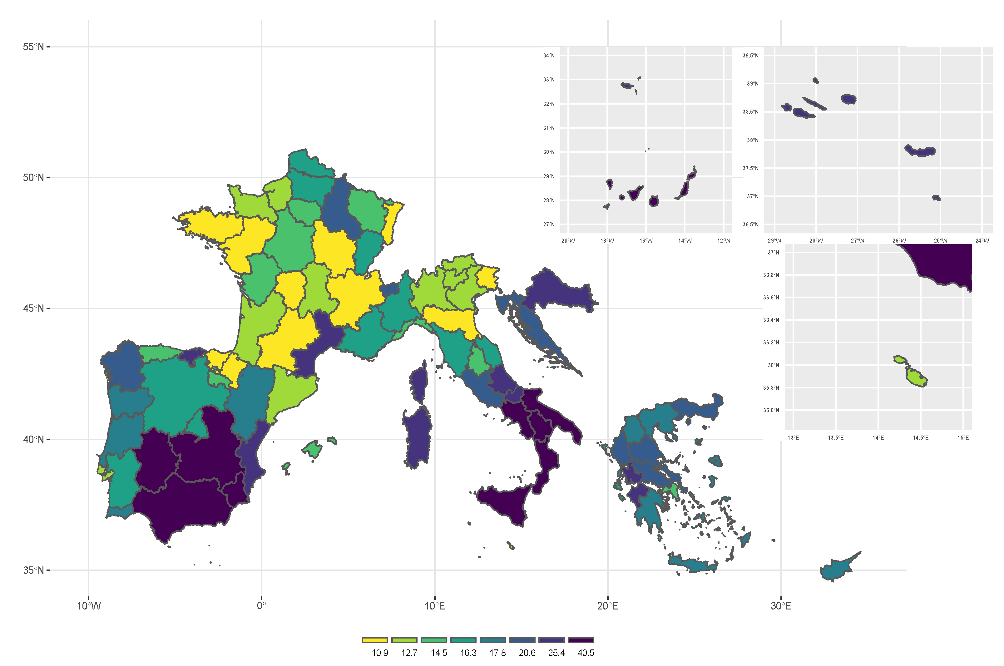
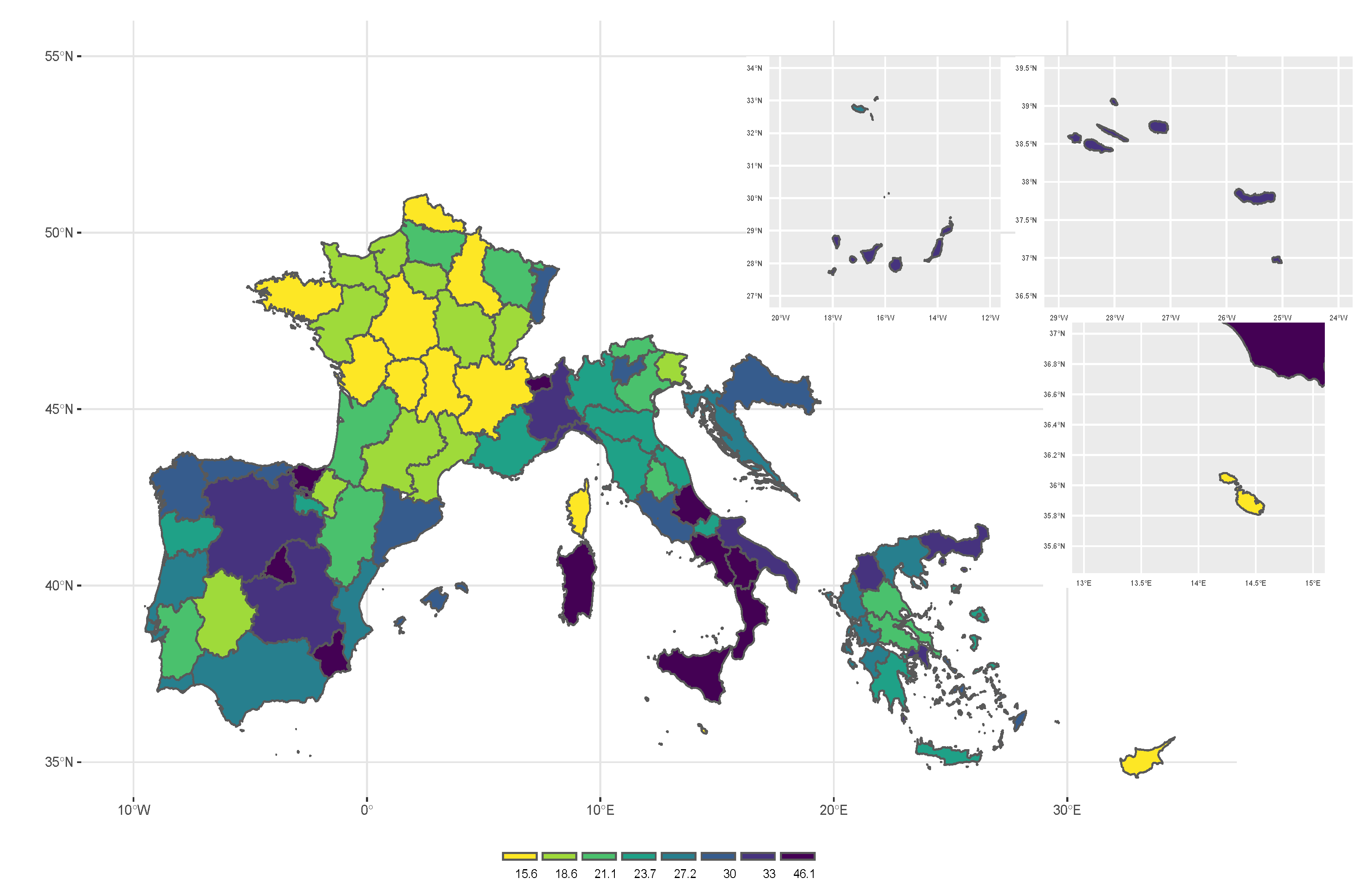
Figure 1 and
Figure 2 and
Table 1 show the distribution of AROP and RMPG in the Mediterranean area. At national level, the highest value for the AROP is observed in Croatia (with a value equal to 21.89%), while the highest value for the RMPG is observed in Portugal (with a value equal to 25.18). In most of the EU Mediterranean countries, the estimated values of AROP and RMPG are higher than the EU-27 average (which are respectively equal to 17% and 24.3%).
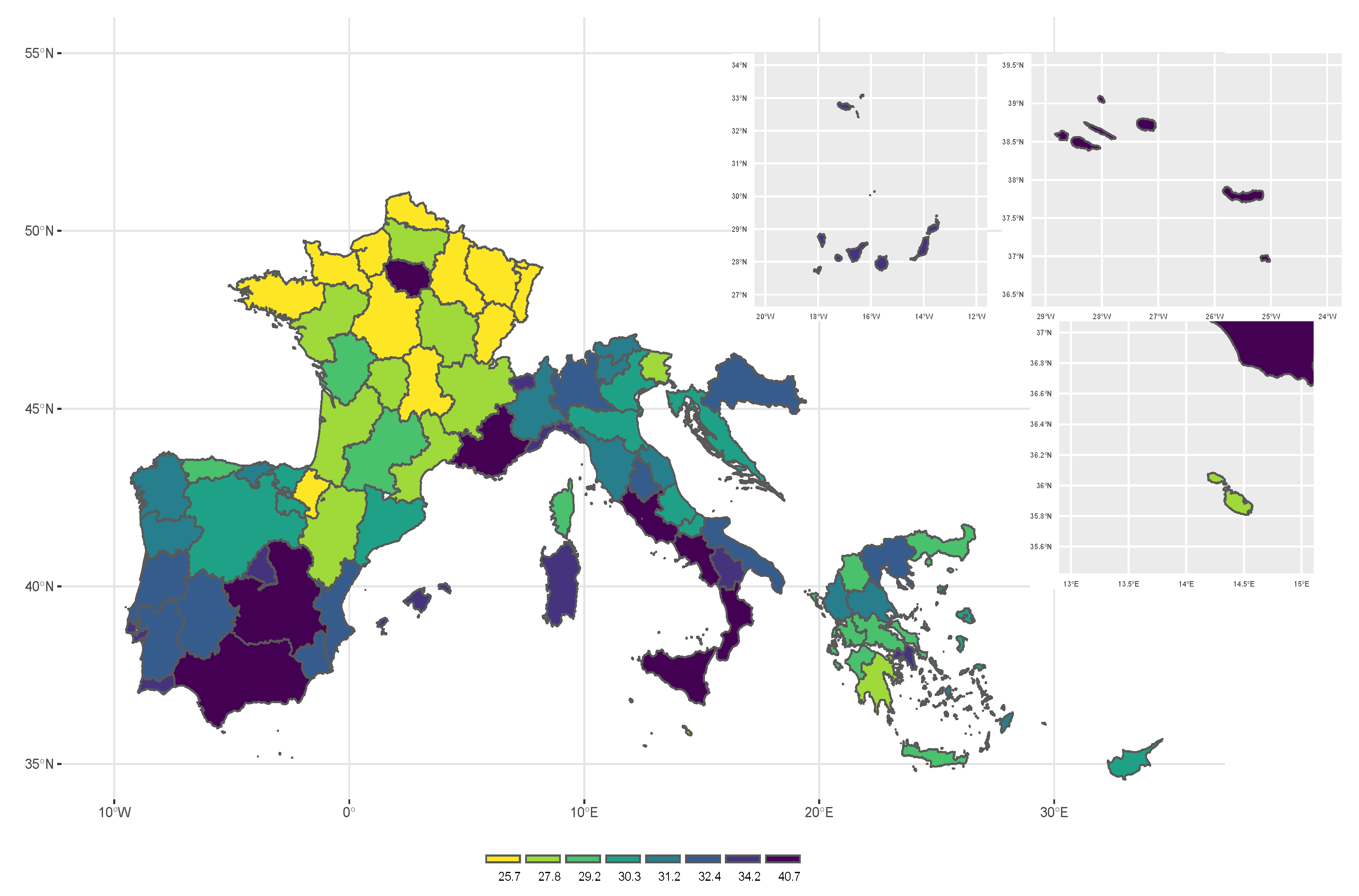
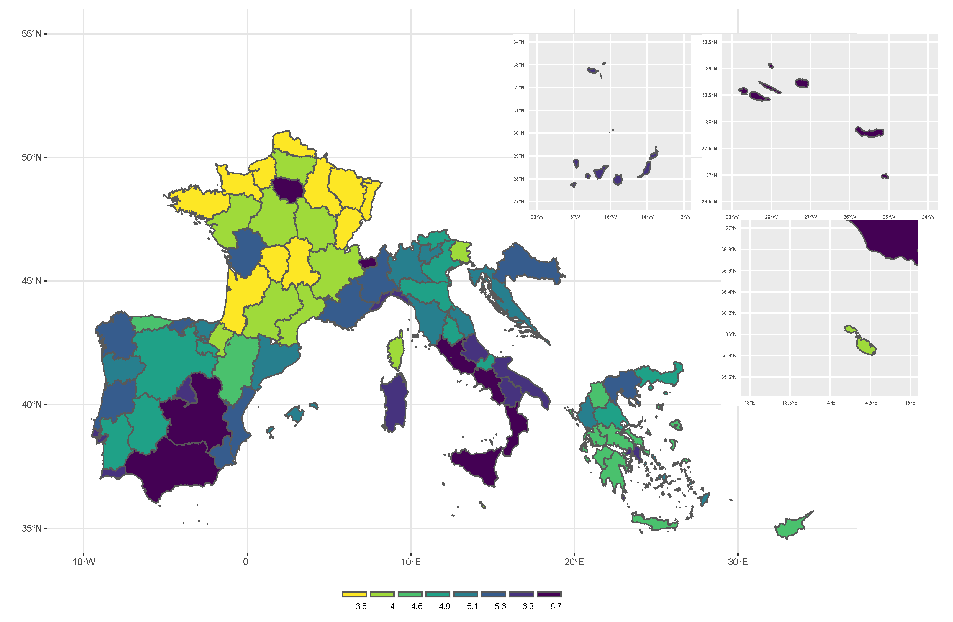
Figure 3 and
Figure 4 and
Table 1 report the distribution of the income-inequality indicators in the Mediterranean area. At national level, the highest values for the S80/S20 and Gini coefficient are observed in Albania, with values respectively equal to 6.7 and 35.28. Overall, Albania, Spain, Croatia, Italy and Portugal report higher values for the income-inequality indicators when compared with the EU-27 average (5.13 for the S80/S20 indicator and 30.8 for the Gini coefficient). It is worth noting that our results show higher values of income-inequality and income-distribution indicators if compared with the official pre-crisis indicators, for example in Spain the AROP in 2008 was equal to 19.8%, while in 2018 it reach a value equal to 20.57%. Similar results are observed in Italy, where the GINI in 2008 was equal to 31.2, while in 2018 it reaches a value equal to 33.3. Focusing on uncertainty measures at national level, it is essential to note that our standard error results show a satisfactory level of reliability, since the estimated coefficients of variation are lower than 5% as underlined by [
57]. Indeed, even if precision thresholds are generally survey-specific and depend on the required reliability and resource-related political decision, specifying what degree of precision is an important step when planning a sample survey.
Turning to estimates at regional level,
Figure 1,
Figure 2,
Figure 3 and
Figure 4 show that national poverty indicators may hide high heterogeneity across regions within each country. As it is known, Cyprus and Malta are not geographically disaggregated at NUTS2 level, while in the case of of Albania, the number of computational units available in the sample is not sufficient to obtain proper estimates via JRR. Therefore for these three countries we can only estimate poverty indicators at national level.
According to
Figure 1, the poorest regions are found in Southern Spain (national poverty line 8918.7) and in Southern Italy (national poverty line 10,280.8). In particular, the area with the highest AROP in Spain is the autonomous city of Ceuta (ES63), situated in the north coast of Morocco. In Italy, the estimated values of the AROP lies between 7.97 in Friuli-Venezia Giulia region and 40.45 in the Campania region. The dualism between North and South of Italy is not confirmed when the RMPG is considered. Indeed, the highest value is observed in Valle d’Aosta with a value equal to 56.068 followed by Abruzzo (38.82) and Sicily (34.49). Similarly, Southern Spain thus not show the highest values which are registered for the autonomous city of Ceuta (45.17), Basque Country (43.56) and Comunidad de Madrid (33.78).
Regarding income-inequality indicators, the highest values for Gini coefficient and S80/S20 are found in Albania (35.28 and 6.7 respectively), Italy (33.33 and 6.08 respectively) and Portugal (33.57 and 5.59 respectively). Also in this case, high national rates are accompanied by concentration of poverty in specific regions. In Italy the estimated values of the GINI lies between 25.68 in Friuli-Venezia Giulia region and 36.02 in the Sicilia region. Similar results are found for S80/S20. In Portugal, the highest value of the who income-inequality indicators are found in the autonomous region of Azores, it is an archipelago composed of nine volcanic islands in the Macaronesia region of the North Atlantic Ocean (38.09 for Gini coefficient and 7.17 for S80/S20). High level of heterogeneity in income-inequality indicators are observed also in Spain: the autonomous city of Ceuta and Melilla (in the north of Africa) show the highest value of the Gini coefficient (40.73 and 38.44 respectively) and S80/S20 (8.67 and 8.34 respectively), followed by the Andalucia region, located in the Southern of Spain, for which the Gini coefficient is equal to 34.93 and the S80/S20 is equal to 6.36. On the contrary, Comunidad Foral the Navarra, located in the Northern Spain, shows the lowest values of these indicators (25.28 for the Gini coefficient and 3.73 for the S80/S20). Moreover, a similar pattern is observed in the case of France. High level of inequality are observed in the Provence-Alpes-Cote d’Azur, in the Southern France, and Ile de France, which is the most populous region of the France and it includes the city of Paris (the Gini coefficient is equal to 34.43 and 34.19); while the lowest values are observed in the Haute-Normandie and Auvergne regions, for which the Gini coefficient is equal to 23.43 and 23.93 respectively.
Looking at the standard errors calculated at national level, it emerges that the RMPG shows higher level of uncertainty compared to the other income-poverty and income-inequality indicators. The relative standard errors for RMPG range from 0.028 in Italy to 0.092 in Cyprus. Contrastingly, the standard errors computed for the AROP show the lowest level of heterogeneity since they range from 0.016 in Italy to 0.056 in Cyprus. This result confirms previous findings ([
8,
16]). It is worth noting that the JRR method can be safely used in the contest of Gini coefficient and the whole family of associated inequality indexes [
31]. The JRR provides stable estimates in particular for cumulative measures such as Gini coefficient and S80/S20 [
8]. The performance of the JRR method for the variance of income-poverty and income-inequality measures is strongly influenced by the type of sample design. Indeed, it has been found that the JRR method works satisfactorily for variance estimation in the case of Gini but not for all sampling designs. The JRR and linearization have been used by [
36] to estimate the variance of the Gini coefficient, allowing for the effect of the sampling design. From
Table 1 can be underlined that there is high variability of uncertainty measures for the various poverty indicators which may be related to the sample design and the size of the sample adopted by each country [
17]. In particular, higher level of standard errors values for the various poverty measures are observed for Cyprus and Malta: a one-stage sampling design have been adopted in Cyprus while a simple random sampling design without have been used by the NSI of Malta. It is worth noting that stratification serves the purpose of increasing the representativeness of the sample and decreasing the risk that sub-groups in the population remain unrepresented. If the variance between strata is large with respect to the relevant variable, stratification contributes to decreasing the standard error. The complexity of the sampling error estimates of these measures is further increased by the fact that the empirical income distribution from which they are derived is itself subject to sampling variability.
As expected, uncertainty measures for income-poverty and income-inequality indicators at NUTS2 level are higher than those obtained at national level. This effect is due to the reduced number of sampling units in each NUTS2 regions. Remarkably, when sample sizes is small, the sampling errors tend to be high. In addition, the estimates of sampling error tend to be more complex and subject to high levels of variability since the number of PSUs in some strata should become smaller with higher level of heterogeneity.
In our analysis some aspects of sample structure have been redefined in order to make variance computation possible, efficient and stable. Due to the unavailability of detailed information regarding the order of unit selection, we had to regroup units by considering individual ID in order to meet the basic requirement of practical methods of variance estimation for complex samples. Sometimes non-response can result in the disappearance from the sample of whole PSUs. This can disturb the structure of the sample, such as increasing the heterogeneity of the PSUs in some strata.
Moreover, it is worth noting that the obtained relative standard errors with the JRR are lower for the income-inequality than those obtained for the income-poverty indicators for all the Mediterranean countries included in our analysis. More specifically, the JRR method provides high standard errors value for the RMPG indicator. Indeed, the relative standard errors obtained using JRR could be affected by the presence of outliers in the income distribution. In order to ameliorate the problem of small sample sizes and produce regional estimates with reduced sampling error, various procedures can be implemented. It is advisable to improve size and unit allocation. The results of this study provide a basis for further statistical developments in the estimation of uncertainty measures including the possibility of using small area estimation methods for obtaining regional estimates with reduced sampling errors [
58].
In addition, in order to improve the measurement of regional poverty and its uncertainty, we will introduce the price dimension into the definition of poverty indicator. More specifically, adjusting the poverty threshold for regional price level differences is essential in order to better assess regional disparities, thus enabling policy makers to adequately identify and address areas of intervention. Indeed, regional values of economic indicators such as Gross Domestic Product (GDP), income and poverty levels, should be adjusted for regional price differences, following the same logic according to which the economic well-being of different countries is compared by taking into account international purchasing power parities ([
59,
60,
61]).
6. Conclusions
This paper addresses the issue of measuring poverty indicators at national and regional level on Mediterranean EU countries by using 2018 EU-SILC surveys. We produced information about the sampling variability of point estimates, which is essential when comparing poverty indicators among geographical areas. We focused on Mediterranean countries, chosen according to their sampling designs.
By considering the income-poverty indicators, our results reveal that at national level, the highest value for the AROP is observed in Croatia (with a value equal to 21.89%), while the highest value for the RMPG is observed in Portugal (with a value equal to 25.18). For income-inequality indicators, the highest value for Gini coefficient and S80/S20 are found in Albania (35.28 and 6.7 respectively), Italy (33.33 and 6.08 respectively) and Portugal (33.57 and 5.59 respectively). Focusing on regional estimates, our estimation results reveal that national poverty indicators may hide a higher heterogeneity of poverty across regions within each country. In particular, high level of heterogeneity is observed in Italy and Spain. The higher level of income-poverty and income-inequality indicators in Mediterranean European countries highlight the problem of insufficient funding of social policies as already introduced by [
62]. In most of the EU Mediterranean countries, the estimated values of the income-poverty indicators are higher than the EU-27 average (which are respectively equal to 17% and 24.3%). Moreover, it is worth noting that our results show higher values of income-inequality and income-distribution indicators if compared with the official pre-crisis indicators, especially for Italy where the GINI in 2008 was equal to 31.2, while in 2018 it reaches a value equal to 33.3. This trend suggests a negative effect on individual welfare and evidence of an increasing trend in inequality in the post-crisis period. By considering the two income-poverty indicators: poverty incidence (AROP) and poverty intensity (RMPG) together, it is possible to obtain a clear indication of the economic well-being of a country [
48]. Focusing on these indicators calculated at sub-national level, it is possible to observe a positive correlation among the Italian regions (with a coefficient of correlation equal to 0.61). The same result is observed for the Portugal regions (with a coefficient of correlation equal to 0.60). These findings prove that these countries are characterized by a high number of poor and with high intensity of poverty. The positive correlation between these two poverty measures produces a picture of the performance of the welfare regimes adopted by these Mediterranean Countries [
48]. These countries share a lower level of social protection in reducing poverty levels, approached by the expenditure on social protection, than the other Mediterranean countries [
63]. In particular, four main traits characterised the Mediterranean welfare state: the low redistributive effect of social transfers and taxes; the bias of the social transfer system towards the risks of elderly people as opposed to the risks of infancy and youth; and the high levels of poverty risks, associated with poor development of minimum income schemes. In these two countries, policy makers need to search for original and better-fitting solutions that acknowledge and shape societies’ values and institutions. Despite in recent years these countries have followed a common path of welfare reforms, weak results have been obtained in poverty reduction. Possible explanations of enduring poverty may include cultural and institutional factors, high levels of tolerance of inequality and poverty. To tackle inequality and promote opportunities for all, countries should adopt a comprehensive policy package, centred around four main areas: promoting greater participation of women into the labour market; fostering employment opportunities and good quality jobs; strengthening quality education and skills development, and adaptation during the working life; and a better design of tax and benefits systems for efficient redistribution.
Turning to the standard error estimates, the JRR method are used for obtaining relative standard errors according to its properties. This method is simpler technically. However, it requires the specification of the sample structure and the appropriate definition of ‘computational PSUs’. It involves repeated computation of the estimates (for which sampling errors are required) over different (often numerous) sample replications. Then variance of any statistic is estimated simply from variability in the estimate itself across the replications and the final variance estimation formula does not depend on the particular statistic involved. Moreover, in order to obtain strata containing at least four PSUs, we have manipulated the data by constructing computational strata.
From our results we can observe that JRR method performs well in the case of income-inequality indicators (Gini coefficient and S80/S20) especially in the case of the Greece, Italy Croatia and Portugal. The estimation results may be influenced by the two-stage sampling design adopted by those countries. By using the JRR method, we are able to better capture both the reduced number of PSUs and, to some extent, the implicit stratification by defining computational strata.
As expected, uncertainty measures for income-poverty and income-inequality indicators at NUTS2 level are higher than those obtained at national level. This effect is due to the reduced number of sampling units in each NUTS2 regions which characterize countries. In addition, when sample sizes become small, sampling error tends not only to be high, but also estimates of sampling error tend to be more complex and subject to high levels of variability. Our findings provide a basis for further research focused on two main directions: implementation of small area estimation methods and computation of poverty indicators adjusted for differences in cost of living among different geographical areas.


