1. Introduction
Intersections are the bottlenecks in the urban roadway network. As traffic demand increases, there is a growing congestion problem at urban intersections. Short-term traffic flow forecasting is crucial for advanced trip planning and traffic management, especially for the highly congested and densely signalized urban roadways. The presence of signalization gives traffic a Spatio-temporal behavior that is more random and difficult to study than in freeways [
1]. In addition, traffic flow in urban signalized arterials has a certain temporal and spatial behavior that exhibits randomness which escapes the traditional perception of periodicity (monthly, weekly, daily, or even hourly periodicities) in traffic operations [
2].
Traffic flow forecasting can be classified into long-term and short-term forecasting. Long-term forecasting usually targets one or more whole days in the future. Short-term models forecast the traffic in the near future (such as a few minutes) based on current and past traffic conditions. It can provide the basis for optimal trip planning, route guidance, and adaptive traffic signal control, and other advanced traffic management schemes. This study focuses on short-term traffic forecasting for signalized intersections. By reviewing the existing methods, it is noticed that some methods can predict short-term traffic flow effectively but cannot adapt well to large scale data processing. Some methods take all the historical data as the input for forecasting instead of selecting a subset of data that is more likely to have a similar pattern as the target day for forecasting, which will have negative impacts on the prediction accuracy and efficiency. In addition, most of the existing methods have only been applied for predicting traffic flow in a very short period, such as one minute or five minutes, which is often too late given that a driver may well be approaching the bottleneck already. For advanced trip planning and traffic management purposes, a model that can forecast the traffic conditions about a half-hour in advance is needed. Therefore, the performance of the existing methods in predicting traffic flow in a longer time window needs to be investigated.
For this purpose, in this study, four representative existing methods, i.e., clustering, k-nearest neighbor algorithm (KNN), backpropagation (BP) neural network, and Elman neural network methods, are selected and applied for predicting the traffic flow condition at a signalized intersection in half-hour advance. In addition, a new model is developed by combining two existing methods: (1) KNN and (2) Elman Neural Network. The performance of the proposed new model is evaluated by comparison with the four selected existing methods.
At first, data collection at a real-world intersection that is used for model development and evaluation is described. Then, four existing short-term traffic flow forecasting models, and the proposed model are introduced and developed using the data collected. Next, the performances of the developed models are evaluated by comparing the forecasted traffic flow rates with real-world observations. Finally, conclusions and recommendations are provided.
2. Literature Review
To predict the short-term traffic flow, many existing models have been developed by previous researchers with different approaches. Generally speaking, the existing methods can be classified into three categories: statistical methods, machine learning methods, and integrated methods combining two or more models.
Statistical models include the historical trend models [
3], nonparametric regression models [
4,
5,
6], and time-series models [
6,
7,
8,
9,
10,
11].
Machine learning models include clustering-based methods [
12], neural network models [
13,
14,
15,
16,
17,
18,
19], Kalman filter models [
20], support vector machine models [
21,
22], decision tree-based methods [
22,
23,
24,
25] and so on. With more and more traffic data available recently, many other machine learning models have been developed. For example, researchers built a deep architecture model stacked with an autoencoder model to predict traffic flow [
26].
Integrated methods (or hybrid methods) have become more popular recently with promising results. Examples include combining some clustering methods with either time-series analysis or neural network models [
17,
27,
28,
29,
30], combining backpropagation (BP) neural network with the radial basis function (RBF) neural network [
31].
Some researchers compared the different approaches for short-term traffic flow forecasting. Smith and Demetsky [
13] compared the historical average, time-series, neural network, and nonparametric regression models, and found that the nonparametric regression model significantly outperformed the other models. Salotti et al. [
32] evaluated ten forecasting methods based on real-world city traffic data in two different contexts. They found the nonparametric approach (KNN) always outperforms other parametric methods in the particular city centre context, while parametric approaches perform better in the freeway context.
By reviewing the existing methods, it can be seen that, for the signalized urban roadways, nonparametric regression models often outperform the traditional time series methodologies due to the rapid variations of traffic flow in urban areas [
1,
33]. Also, KNN regression model has been widely used for short-term traffic flow forecasting and has been reported to have good performance [
34,
35,
36,
37]. In addition, it also has been reported that neural network models have many advantages over the classical statistical methods in short-term traffic flow forecasting [
38]. Furthermore, many previous studies have used clustering-based methods in traffic flow forecasting and have shown improved modeling performance [
12,
39]. Therefore, in this study, a representative nonparametric regression model, i.e., KNN regression model, a clustering-based algorithm, and two neural network models were selected for comparing with the proposed integrated model.
3. Data Description
A signalized intersection in Jinan, China was selected as the study intersection. At this site, 156 days of traffic data were collected, from 1 October 2018 to 1 April 2019. Multi-dimensional data was collected, including:
Since the central data collection devices and management system are scheduled for regular maintenance on every Tuesday, so there is no data available on Tuesday. Also, since the signal cycle length is 1.5 min in some periods and is 2 min in other periods, for uniformity, the cycle by cycle traffic flow data is aggregated at a 6-min interval level. Thus, the traffic flow rate in this study is the number of arrival vehicles per 6 min. After examination, it was found that there were many missing data from 21 to 29 November 2018, so these 9 days were removed. In addition, in some days, the data were missing for more than 3 consecutive time intervals (18 min). These data were also excluded from this study. For the data missing less than 18 min, for data imputation purposes, the average traffic flow rates before and after it were used as the estimated traffic flow rates for these time intervals.
The data were then divided into two sets, training dataset and validation dataset. In this paper, 6 days’ data from 27 March to 1 April were used for model validation, and the rest of the data were used as training data for model development. In addition, all data were also classified into three groups: weekdays, weekends and holidays. Since there are only a few holidays during the study period, all the data collected during the holidays were excluded. Finally, only two groups of data, i.e., weekday and weekend, were included in both training and validation datasets.
4. Methodology
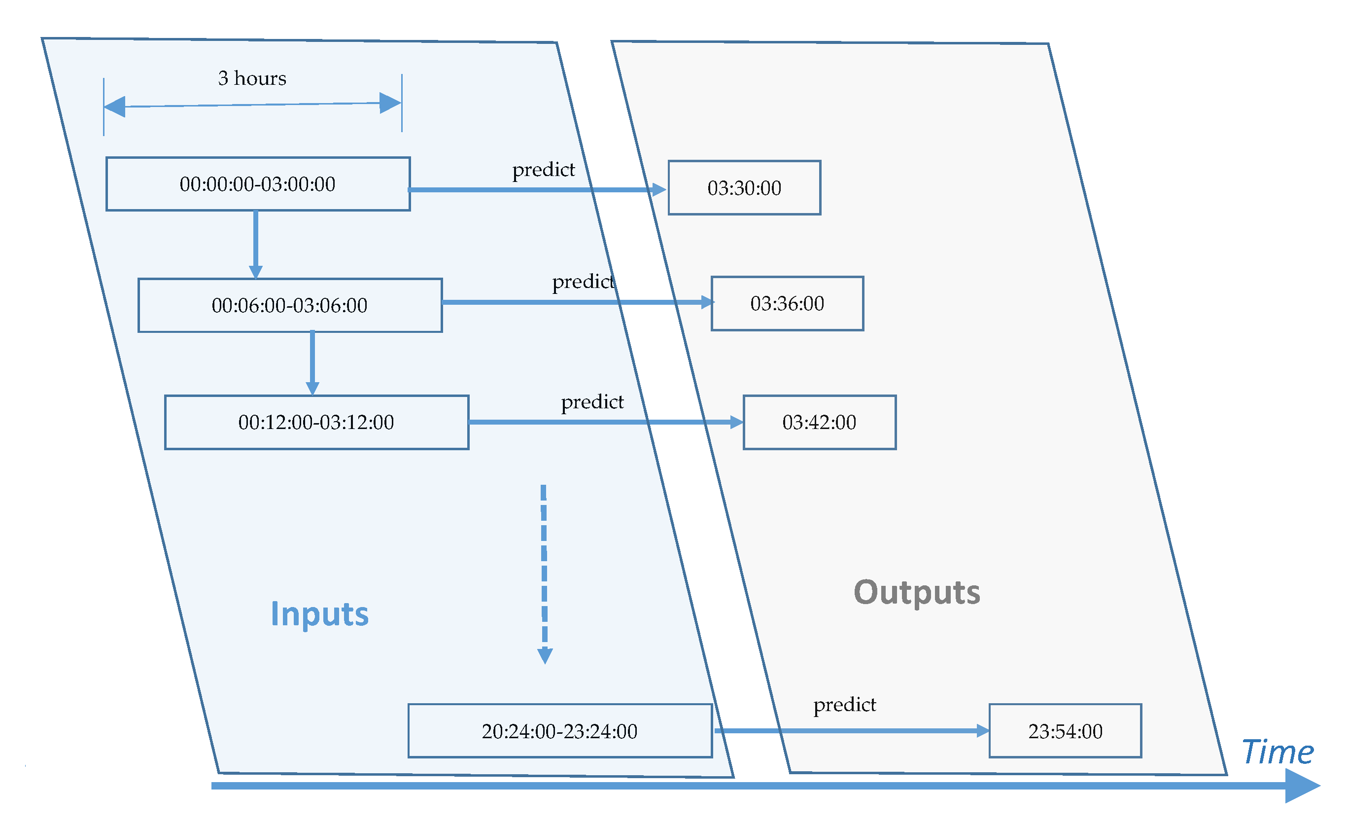
In this study, the short-term intersection traffic flow forecasting model is for predicting the amount of traffic that will arrive at an intersection 30 min later based on the arriving traffic flow rates during the past 3 h. Thus, mathematically, the model can be expressed by the following equation.
where
t is the current time interval and
is the arrival traffic flow rate during the current time interval. Since the traffic flow rate is at a 6-min interval, the vector
represent the arrival travel flow rates during the past 3 h and
represent the predicted rate of the traffic flow that will arrive at the intersection after half an hour.
Figure 1 shows the inputs and outputs of the developed models.
In this paper, four existing methods are considered for developing the short-term intersection traffic flow forecasting models. They are clustering, k-nearest neighbor algorithm (KNN), backpropagation (BP) neural network and Elman neural network methods. In addition, by integrating the KNN and Elman methods, a two-layer stacking model is also developed. These models will be introduced one by one in the following sections.
4.1. Clustering Method-Based Algorithm
Clustering is one of the most important unsupervised data mining methods. It groups a set of objects in such a way that objects in the same group (called a cluster) are more similar (in some sense) to each other than to those in other groups (clusters). A classic definition for clustering is described as follows [
40,
41]:
Instances, in the same cluster, must be similar as much as possible;
Instances, in the different clusters, must be different as much as possible;
Measurement for similarity and dissimilarity must be clear and have practical meaning.
In this study, a novel density-based clustering method developed by Rodriguez and Laio [
42] was used to divide the historical traffic flow data into different groups. A detailed introduction about this clustering method can be found in Song et al. [
39]. In this study, the clustering method is used to find all the historical traffic flow records during the given period and in a given type of day (weekday or weekend) that have a similar traffic pattern as the target day. The period is 3 h before the current time
t. To develop the clustering model, all the 3-h traffic flow vectors
were derived from the collected traffic data. Then, these vectors are divided into different groups according to the type of day (weekday or weekend) and the time of the day (
t).
The similarity between the traffic flow data during the same 3-h period in different days was defined by the Euclidean distance as follows
where
i and
j indicate different days, t is the current time interval and
is the arrival traffic flow rate during the time interval
t −
k in Day
i.
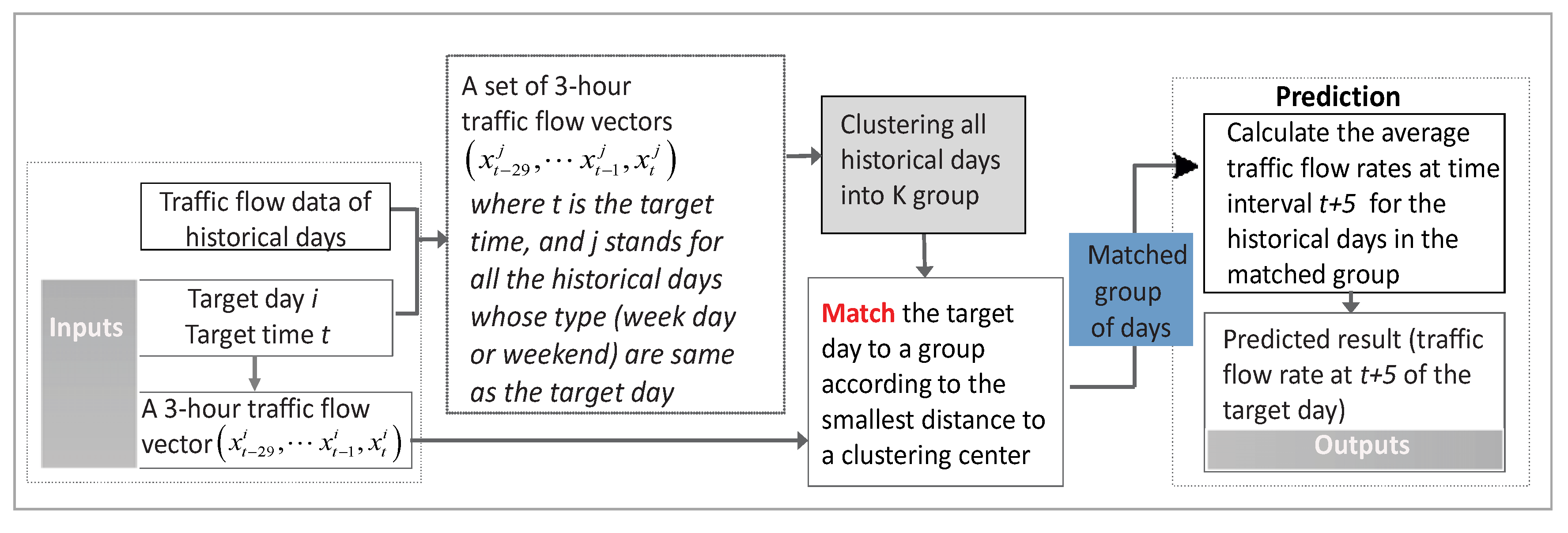
The general framework of the clustering-based algorithm is presented in
Figure 2. Given a target day
i and a target time
t, we will know the 3-h traffic flow condition before this time. Then, by applying the clustering method to the corresponding historical traffic flow vector group, the historical days that have a similar traffic pattern as the target day during the same 3-h period on the same type of day of the week can be identified. Then, by calculating the average traffic flow rates at time interval
t + 5 (30 min after the target time
t) in these identified days, the traffic flow rate for the target day 30 min after the target time
t can be predicted.
4.2. K-Nearest Neighbor’s Algorithm (KNN)
KNN is a non-parametric method that can be used for classification and regression. In this study, KNN was used for regression. The core idea for the KNN regression is to find the k nearest neighbors of a given set of inputs and use the average values of the k nearest neighbors as the outputs of the model. In this study, the input for the KNN model is the 3-h traffic flow vectors of the target day at a given time t. To identify the k nearest neighbors for the inputs, the distance between this input and the samples in the training data needs to be defined at first. In this study, the Euclidean distance given in Equation (2) is also used for defining this distance. Similar to the Clustering method, the KNN method also aims to find out all the historical traffic flow records that have a similar pattern to the target day in a given time period and a given type of day (weekday or weekend), so as to predict the traffic flow rate in the next half hour for the target day. The only difference is that the Clustering method identifies all the traffic flow vectors in the same clustering group, while the KNN method only identifies the k most similar records that are closest to the inputted traffic flow vectors.
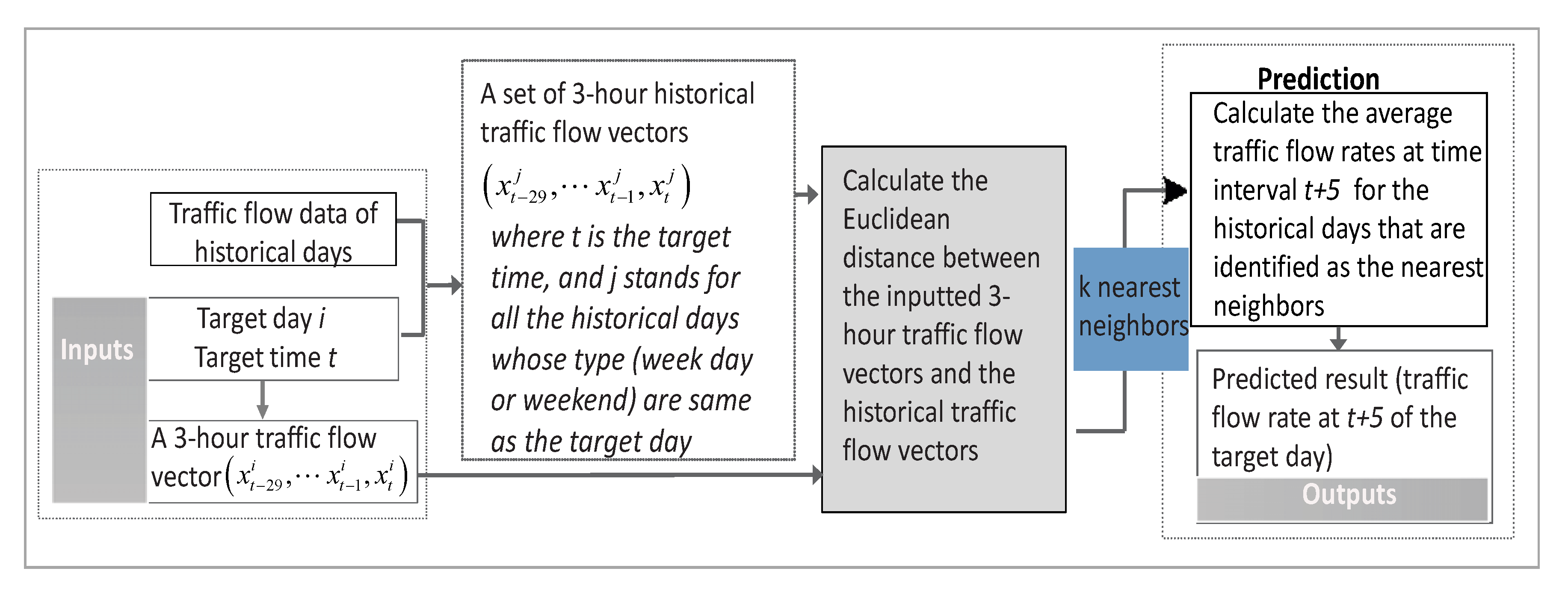
The general framework of the KNN model is presented in
Figure 3. Basically, the KNN algorithm consists of the following key steps:
- (1)
For a given target day i and a target time t, find the correspondent training dataset that contains historical traffic records (3-h traffic flow vectors) during the same type of days (weekday or weekend) at the target time t
- (2)
Calculate the distance between the inputted 3-h traffic flow vectors and the traffic flow vectors in the training dataset according to the Euclidean distance given in Equation (2).
- (3)
Select the k traffic flow vectors with the smallest distances
- (4)
According to the date and time of the selected traffic flow vectors, calculate the average traffic flow rate in these k days half an hour after the given time t, which will be the forecasted traffic flow rate for the target day i 30 min after the target time t.
4.3. Backpropagation (BP) Neural Network
The BP neural network algorithm is one of the most widely applied neural network models and has been applied for traffic flow forecasting in some previous studies [
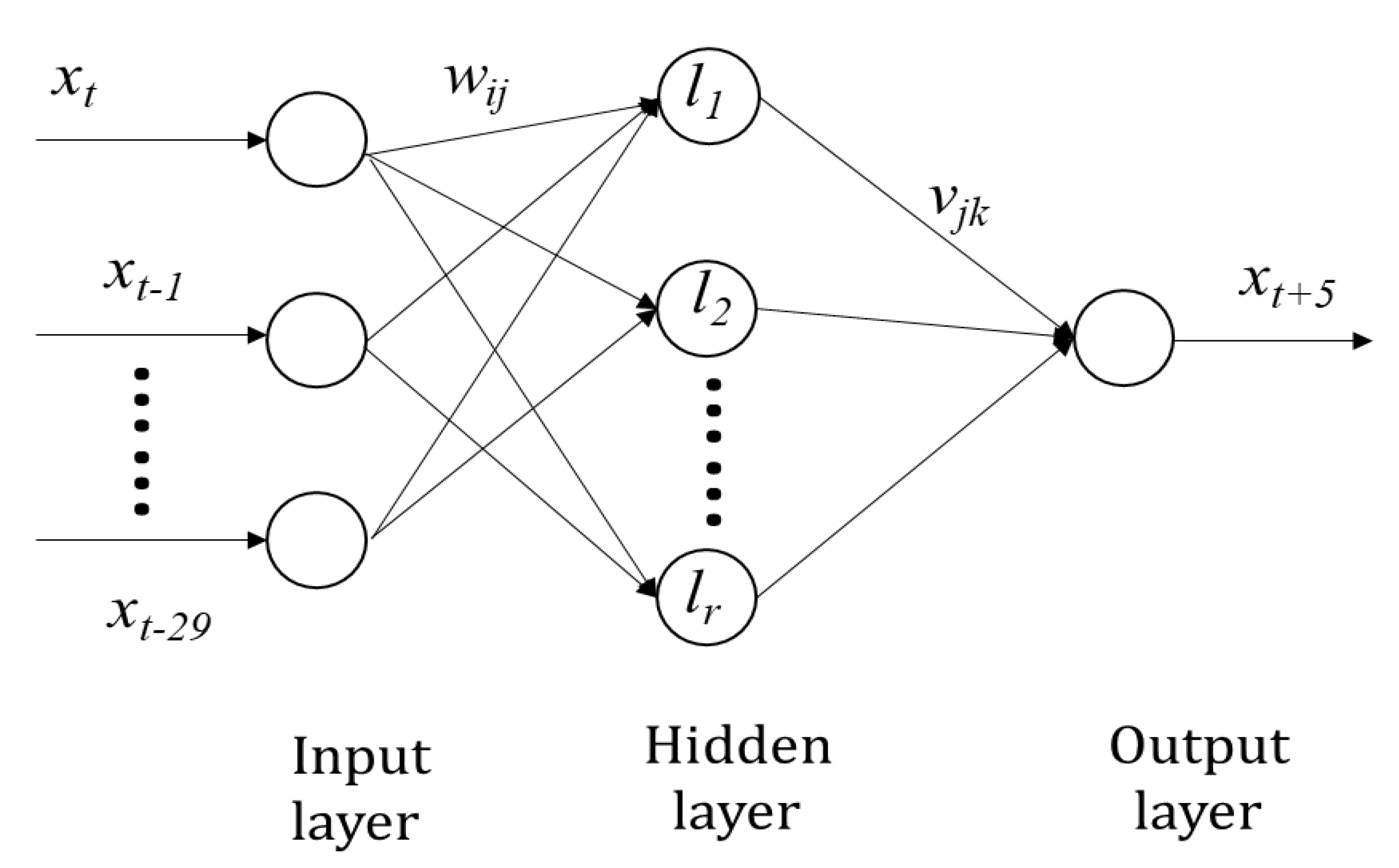
31]. In this study, a BP neural network is selected with three layers: (1) an input layer, (2) a hidden layer, and (3) an output layer. The overall structure of the BP neural network is presented in
Figure 4. In this structure, there are 30 neurons in the input layer, i.e.,
which represent the 3-h traffic flow rate vectors and 1 neuron in the output layer, i.e.,
which is the traffic flow rate in half an hour;
wij is the weight for the connection from neuron
i in the input layer to neuron j in the hidden layer, and
vjk is the weight for the connection from neuron
j in the hidden layer to neuron
k in the output layer. The training of the BP model was based on the backpropagation method. In this study, the transfer function for the neurons in the hidden is chosen as the sigmoid function and the transfer function for the neurons in the output layer is a linear function.
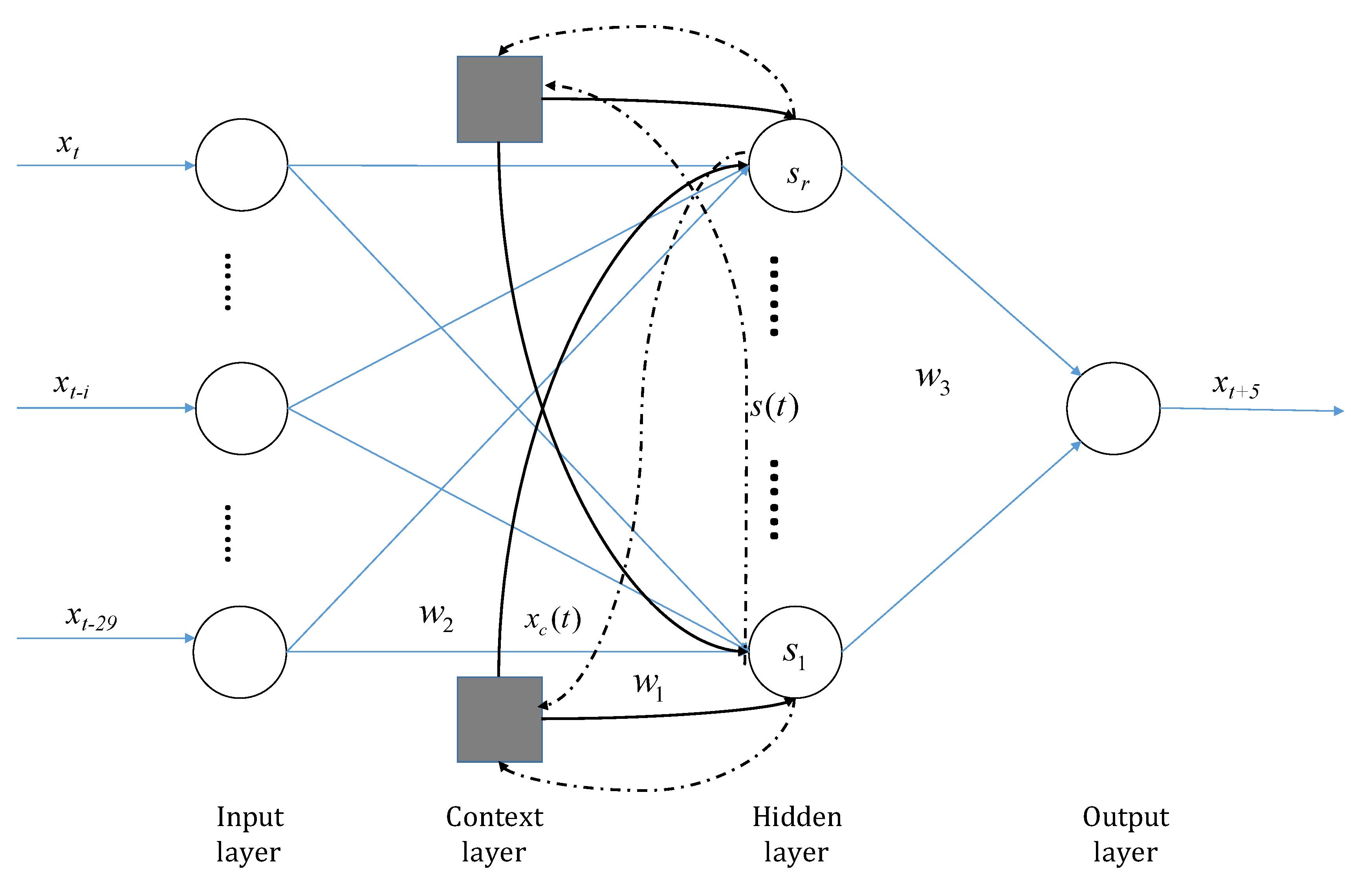
4.4. Elman Neural Network
Elman neural network is a dynamic feedback neural network, which was proposed by Elman in 1990 for voice processing. Several previous studies have been conducted to develop short-term traffic flow forecasting models based on Elman neural network [
18,
29,
43]. The Elman neural network is generally considered to be a forward neural network with local memory units and local feedback connections. Its main structure is similar to the structure of BP neural network, but it adds a context layer to the hidden layer based on the basic structure of BP neural network. The context layer mainly receives feedback signals from the hidden layer as a delay operator. It was used to memorize the output value of the hidden layer neuron at the previous moment. Thus, the output of the context layer neuron is stored and then inputted to the hidden layer. It enhances the model’s ability to process dynamic information.
In this study, a simple three-layer Elman network was adopted.
Figure 5 shows the structure of the Elman network. The relationships between the neurons in different layers of the network can be expressed as:
where,
t represents time and
y, s,
x,
xc represent the output neuron vector, hidden layer neuron vector, input neuron vector, and context neuron vector, respectively.
is the connection weight matrix from the hidden layer to the output layer,
is the connection weight matrix from the input layer to the hidden layer, and
is the connection weight matrix from the context layer to the hidden layer, respectively.
f(.) is the transfer function of the hidden layer neurons, using the tansig function, and
g(.) is the output layer transfer function, using the tansig function. In this study, the Elman neural network uses the optimized gradient descent algorithm for training. Through learning and training, the difference between the actual output value and the output value of the network is used to continuously modify the weights and thresholds, so that the sum of squares of errors at the output layer of the network is minimized.
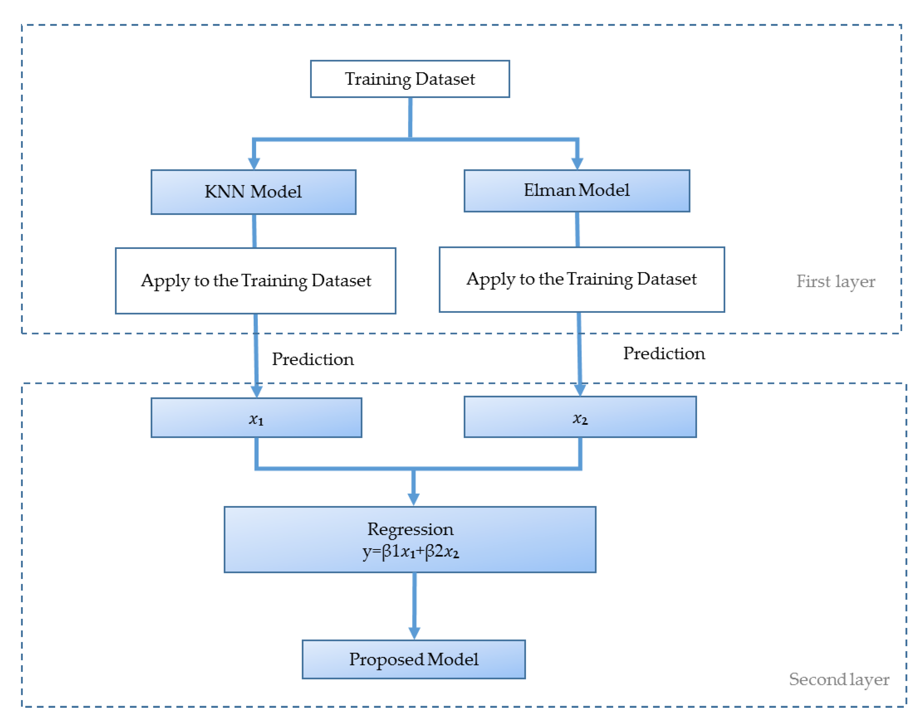
4.5. A Two-Layer Stacking Model
An individual prediction model often has its limitations, so integrating different forecast models in accordance with a proper form can comprehensively utilize all kinds of information provided by them and they can learn from each other so as to effectively improve the prediction accuracy, which is the concept of combinational forecast [
44]. According to this idea, this study is to develop an integrated model that can combine the strengths of the existing models. To this end, we compared the four existing modeling methods introduced earlier. First, the clustering model was compared with the KNN model because they are developed based on similar ideas and all belong to the nonparametric regression models. According to some existing studies [
45,
46,
47], the KNN model shows better performance than the clustering models. Thus, in the study, the KNN is selected for developing the integrated model. Second, the BP model was also compared with the Elman model because both are neural network models. Theoretically, the Elman model should have better performance than the BP model because it enhanced the BP model by adding a context layer that feeds back the hidden layer outputs in the previous timesteps. The advantages of the Elman model have been verified by many existing studies [
48,
49]. Thus, Elman was selected for developing the integrated model. In this study, a two-layer stacking model that integrates KNN and Elman methods is proposed to combine the strengths of both models. The main idea of stacking is to train the individual KNN and Elman models with training data in the first layer, and then use the predictions of both models as input variables for model integration in the second layer [
50].
Figure 6 shows the structure of the proposed stacking model.
As we introduced before, the collected data were divided into two groups, i.e., training dataset and validation dataset. Data collected before 27 March 2019 were used as the training data to train KNN and Elman models separately in the first layer. For the KNN models, it searches for k nearest neighbors (traffic flow vectors) in the training data and uses the average traffic volume (after half an hour) of the identified neighbors as the prediction. It is an algorithm and no specific parameters need to be calibrated. For the Elman model, the connection weight matrixes need to be calibrated using the training data. To develop the second layer regression models, we reapplied the developed KNN and Elman models to the same training dataset to derive the predictions for the samples in the training dataset. Then, the predictions from the KNN and Elman models were used as two independent variables, i.e.,
and
to derive a regression model, in which the observed traffic flow rate is the dependent variable
y. Note that, from
Figure 6, it can be seen that the proposed two-layer stacking model was developed by only using the training dataset. Also, since the traffic patterns are different during different days of the week, different regression models were developed for different days of the week in the second layer (
Table 1). Following are the regression models in the second layer developed from Wednesday through Monday:
Note that, as mentioned before, since the central data collection devices and management system is scheduled for regular maintenance every Tuesday, so there is no data available on Tuesday. Therefore, no model was developed for Tuesday.
5. Model Evaluation
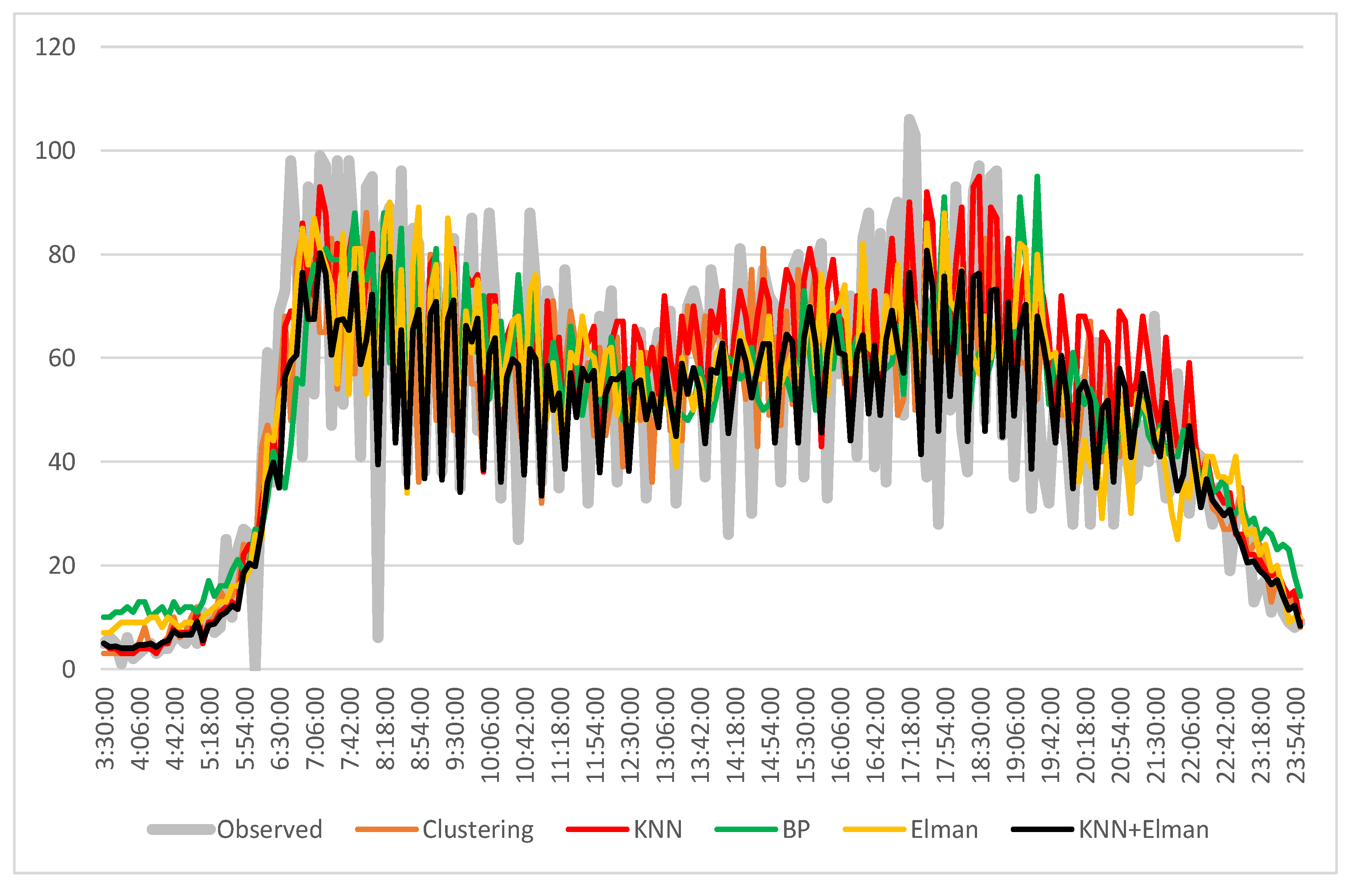
The developed models were applied to the validation dataset, which is to predict the traffic flow rate (number of vehicles per 6 min) during one week from 27 March 2019 (Wednesday) to 1 April 2019 (Monday). The prediction starts at 3:30 a.m. every day because the data collected during the first three hours from 0:00 a.m.–3:00 a.m .were used as the model inputs for the first prediction at 3:30 a.m. Thereafter, as the time window moves, a prediction will be generated every 6 min. As an example, the prediction results for the 1 April are present in
Figure 7.
Figure 7 shows the observed traffic flow and the forecasted traffic flows by different models. It can be seen that KNN performs best sometimes, especially in the afternoon and early evening (12:30 p.m.–6:30 p.m.). However, KNN + Elman performs better than KNN in the morning (8:00 a.m.–10:00 a.m.) and late evening (7:00 p.m.–10:00 p.m.). To compare the overall performance of different models, two quantitative performance measures were used.
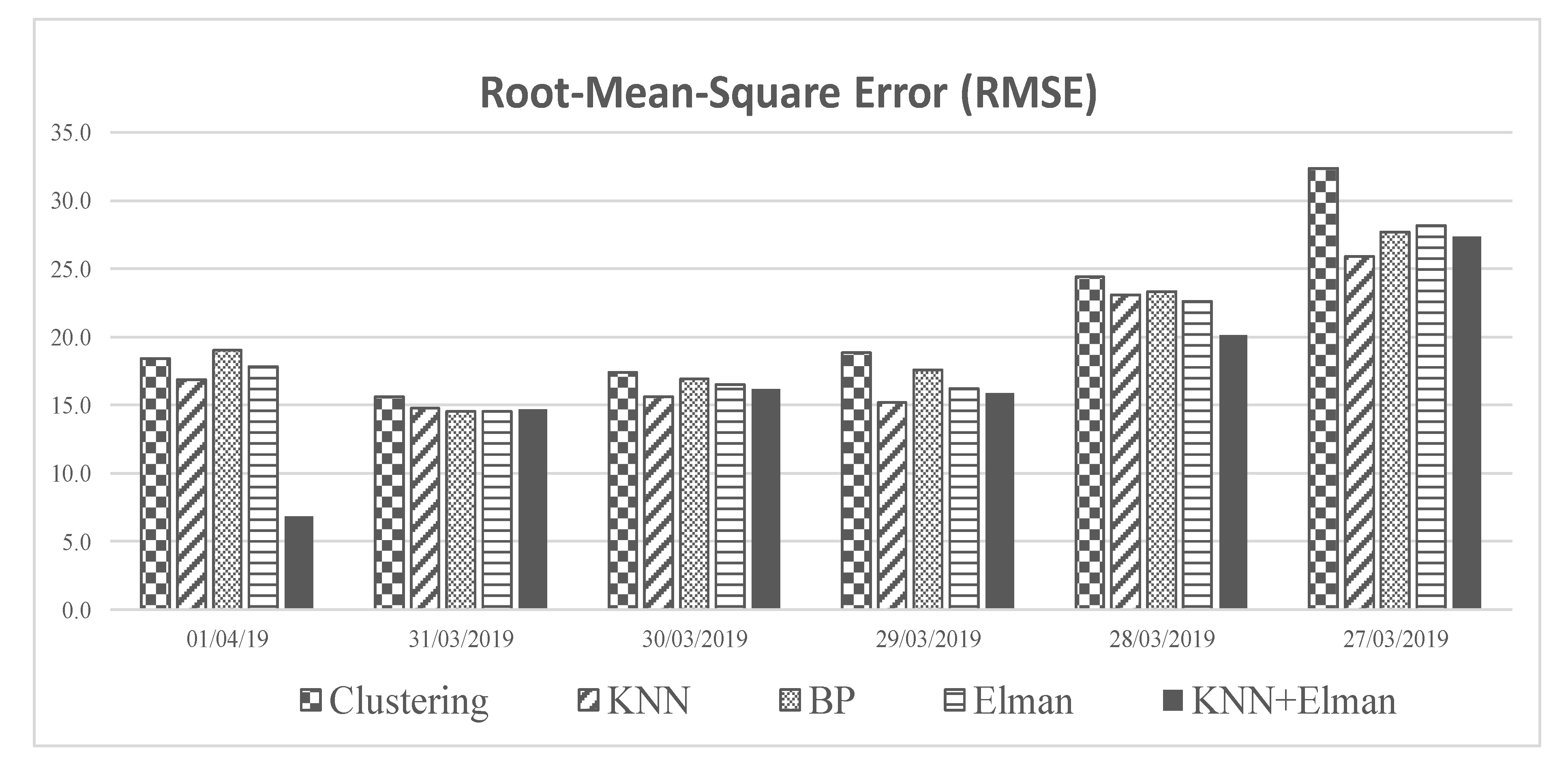
In this study, the prediction accuracies of different models were evaluated by using two measures (1) the Root Mean Squared Error (RMSE), and (2) the Correlation Coefficient between the Predicted and Observed values (CCPO). The RMSE measures the differences between the predicted and observed values, which can be expressed by the following equation:
where,
is the predicted traffic flow rate,
is the observed traffic flow rate and
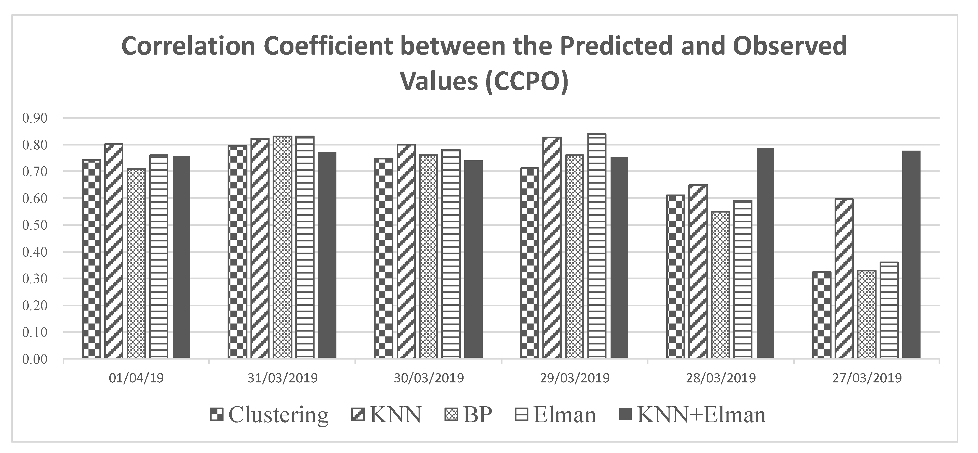
T denotes the total number of time intervals during the prediction period. A lower RMSE value indicates a better prediction. The CCPO measures the correlation between the predicted and observed traffic flow rates (CCPO). A higher CCPO value indicates a better prediction. It is because a high CCPO value means that the predicted values and the observed values have the same trend of change.
According to these two measures, the performances of the developed models are compared and presented in
Figure 8 and
Figure 9.
From
Figure 8 and
Figure 9, it can be seen that the KNN model consistently outperforms the clustering model, which is consistent with the findings in the literature [
46,
47]. Also, by comparing the BP model with the Elman model, it was found that the Elman model has better performance than the BP model in almost all six days. This result also reasonable because the Elman model enhanced the BP model by adding a context layer that feeds back the hidden layer outputs in the previous timesteps. The proposed 2-layer stacking model integrating the KNN and Elman methods has better or close performance than the KNN and Elman models. Overall, the proposed model outperformed all the other four models.
Table 2 lists the overall six-day average performance of these five models in terms of their RMSE and CCPO values. It also clearly shows that the proposed model outperforms the other four models. The evaluation result indicates that the proposed 2-layer stacking model can more accurately forecast the intersection short-term (30 min) traffic flow than the four widely used existing models.
6. Conclusions and Recommendations
In this study, a 2-layer stacking model integrating the KNN and Elman methods is proposed for forecasting intersection short-term traffic flow. A signalized intersection in Jinan, China was selected as a study intersection. Based on the real-world data collected at this intersection, five models were developed, including four widely used existing short-term traffic forecasting models as well as a 2-layer stacking model proposed by this study. To evaluate the performance of the proposed model, all five developed models were applied to the study intersection for forecasting six days’ traffic flow. By comparing the RMSEs and CCPOs of these models, it was found that the proposed model can produce more accurate predictions than the other four models. This research work filled the gaps identified in the introduction part. First, for the proposed model, the KNN model at the 1st layer was developed only based on the historical days that have similar traffic pattern as the target day instead of all the historical traffic flow data. As a result, the developed model can better capture the traffic characteristics of the target day and provide more accurate predictions. Second, in this paper, a new concept of short-term traffic flow prediction is proposed. Different from the most existing traffic flow prediction models, the proposed model was designed for predicting the traffic flow condition in half-hour advance which can better meet the needs of advanced trip planning and traffic management. Note that, due to the data limitation, the developed model cannot be used for predicting the traffic flow conditions on a holiday. In the future, more data need to be collected for both holiday and non-holiday to develop a more comprehensive traffic flow prediction model. In addition, this research only used data collected from one intersection for developing and evaluating the proposed model. In the future, the proposed modeling method can be applied to more locations and using more data for further validation.
Author Contributions
Data curation, D.L. and S.L.; Formal analysis, J.L. and Q.Z.; Investigation, W.Q.; Methodology, W.Q., J.L., D.L., L.Y., S.L. and Y.Q.; Supervision, Y.Q.; Writing—original draft, W.Q.; Writing—review & editing, Q.Z. and Y.Q. All authors have read and agreed to the published version of the manuscript.
Funding
This research was funded partially by the U.S. Department of Transportation: (USDOT), grant number 69A3551747133 and the Department of Higher Education, Chinese Ministry of Education, grant number S202010431014. The APC was funded by Texas Southern University.
Acknowledgments
The authors would like to show our gratitude to Yongxue Liu for her assistance with data collection and programing, and Xiaoran Li and Lei Liu for their assistance with literature search and model validation.
Conflicts of Interest
The authors declare no conflict of interest.
References
- Head, L.K. Event-based short-term traffic flow prediction model. Transp. Res. Rec. 1995, 1510, 45–52. [Google Scholar]
- Stathopoulos, A.; Karlaftis, M.G. Temporal and spatial variations of real-time traffic data in urban areas. Transp. Res. Rec. J. Transp. Res. Board 2001, 1768, 135–140. [Google Scholar] [CrossRef]
- Jiang, Y.; Guo, J.; Zhao, J. Short-term traffic flow’s forecasting by fusing wavelet neural network and historical trend model. Mod. Comput. 2013, 3, 26–29. [Google Scholar]
- Davis, G.A.; Nihan, N.L. Nonparametric regression and short term freeway traffic forecasting. J. Transp. Eng. 1991, 117, 178–188. [Google Scholar] [CrossRef]
- Smith, B.L.; Demetsky, M.J. Short-Term Traffic Flow Prediction: Neural Network Approach. Transportation Research Record 1453; Transportation Research Board: Washington, DC, USA, 1994; pp. 98–104. [Google Scholar]
- Smith, B.L.; Williams, B.M.; Oswald, R.K. Comparison of parametric and nonparametric models for traffic flow forecasting. Transp. Res. Part C Emerg. Technol. 2002, 10, 303–321. [Google Scholar] [CrossRef]
- Ahmed, S.A.; Cook, A.R. Analysis of Freeway Traffic Time-Series Data Using Box-Jenkin Methods; Transportation Research Record: Washington, DC, USA, 1979; Volume 722, pp. 1–9. [Google Scholar]
- Hamed, M.M.; Al-Masaeid, H.R.; Said, Z.M. Short-term prediction of traffic volume in urban arterials. J. Transp. Eng. 1995, 121, 249–254. [Google Scholar] [CrossRef]
- Moorthy, C.K.; Ratcliffe, B.G. Short term traffic forecasting using time series methods. Transp. Plan. Technol. 1988, 12, 45–56. [Google Scholar] [CrossRef]
- Omkar, G.; Kumar, S. Time series decomposition model for traffic flow forecasting in urban midblock sections. In Proceedings of the 2017 International Conference on Smart Technologies for Smart Nation (SmartTechCon), Bangalore, India, 17–19 August 2017. [Google Scholar]
- Williams, B.M.; Durvasula, P.K.; Brown, D.E. Urban freeway traffic flow prediction: Application of seasonal autoregressive integrated moving average and exponential smoothing models. In Transportation Research Record 1644; Transportation Research Board: Washington, DC, USA, 1998; pp. 132–141. [Google Scholar]
- Han, L.; Zheng, K.; Zhao, L.; Wang, X.; Shen, X. Short-term road traffic prediction based on deep cluster at large-scale networks. IEEE Trans. Veh. Technol. 2019, 68, 301–313. [Google Scholar] [CrossRef]
- Smith, B.L.; Demetsky, M.J. Traffic flow forecasting: Comparison of modeling approaches. J. Transp. Eng. 1997, 123, 261–266. [Google Scholar] [CrossRef]
- Zhang, H.J.; Ritchie, S.G.; Lo, Z.P. Macroscopic Modeling of Freeway Traffic Using an Artificial Neural Network; Transportation Research Boarg: Washington, DC, USA, 1997; pp. 110–119. [Google Scholar]
- Dougherty, M.S.; Kirby, H.C. The use of neural networks to recognize and predict traffic congestion. Traffic Eng. 1998, 34, 311–314. [Google Scholar]
- Pamuła, T. Short-term traffic flow forecasting method based on the data from video detectors using a neural network. In Activities of Transport Telematics; Communications in Computer and Information Science; Mikulski, J., Ed.; Springer: Berlin/Heidelberg, Germany, 2013; Volume 395. [Google Scholar] [CrossRef]
- Park, B.; Carroll, J.M.; Urbank, T., II. Short-Term Freeway Traffic Volume Forecasting Using Radial Basis Function Neural Network; Transportation Research Record 1651; Transportation Research Board: Washington, DC, USA, 1998; pp. 39–46. [Google Scholar]
- Zhao, J.; Gao, H.; Jia, L. Short-term traffic flow forecasting model based on elman neural network. In Proceedings of the 27th Chinese Control Conference, Kunming, China, 16–18 July 2008; pp. 499–502. [Google Scholar] [CrossRef]
- Niu, Z.; Jia, Y.; Zhang, L.; Liao, C. Prediction for short-term traffic flow based on elman neural network optimized by CPSO. Geotech. Test. J. 2013, 36, 1–10. [Google Scholar]
- Okutani, I.; Stephanedes, Y.J. Dynamic prediction of traffic volume through kalman filtering theory. Transp. Res. Part B Methodol. 1984, 18, 1–11. [Google Scholar] [CrossRef]
- Fu, G.; Han, G.; Lu, F.; Xu, Z. Short-term Traffic Flow Forecasting Model Based on Support Vector Machine Regression. J. South China Univ. Technol. Nat. Sci. Ed. 2013, 41, 71–76. [Google Scholar]
- Wang, D.; Zhang, Q.; Wu, S.; Li, X.; Wang, R. Traffic flow forecast with urban transport network. In Proceedings of the IEEE International Conference on Intelligent Transportation Engineering, Singapore, 20–22 August 2016. [Google Scholar]
- Liu, Y.; Wu, H. Prediction of road traffic congestion based on random forest. In Proceedings of the10th International Symposium on Computational Intelligence and Design, Hangzhou, China, 9–10 December 2017. [Google Scholar]
- Xia, Y.; Chen, J. Traffic flow forecasting method based on gradient boosting decision tree. In Proceedings of the 5th International Conference on Frontiers of Manufacturing Science and Measuring Technology (FMSMT), Taiyuan, China, 24–25 June 2017. [Google Scholar]
- Yang, S.; Wu, J.; Du, Y.; He, Y.; Chen, X. Ensemble learning for short-term traffic prediction based on gradient boosting machine. J. Sens. 2017. [Google Scholar] [CrossRef]
- Lv, Y.; Duan, Y.; Kang, W.; Li, Z.; Wang, F. Traffic flow prediction with big data: A deep learning approach. IEEE Trans. Intell. Transp. Syst. 2015, 16, 865–873. [Google Scholar] [CrossRef]
- Kuchipudi, C.M.; Chien, S.I. Development of a hybrid model for dynamic travel-time prediction. Transp. Res. Rec. 2003, 1855, 22–31. [Google Scholar] [CrossRef]
- Liu, Z.; Guo, J.; Cao, J.; Wei, Y.; Huang, W. A Hybrid Short-term Traffic Flow Forecasting Method Based on Neural Networks Combined with K-Nearest Neighbor. Available online: https://traffic.fpz.hr/index.php/PROMTT/article/view/2651 (accessed on 20 June 2020).
- Song, X.; Li, H.; Wu, B.; Li, A. Elman neural network model of traffic flow predicting in mountain expressway tunnel. In Proceedings of the 2010 International Conference on Computational Intelligence and Software Engineering, Wuhan, China, 10–12 December 2010; pp. 1–4. [Google Scholar]
- Yin, H.; Wong, S.; Xu, J.; Wong, C. Urban traffic flow prediction using a fuzzy-neural approach. Transp. Res. Part C Emerg. Technol. 2002, 10, 85–98. [Google Scholar] [CrossRef]
- Zheng, W.; Der-Horng Lee, M.; Shi, Q. Short-term freeway traffic flow prediction: Bayesian combined neural network approach. J. Transp. Eng. 2006, 132, 114–121. [Google Scholar] [CrossRef]
- Salotti, J.; Fenet, S.; Billot, R.; Faouzi, N.E.; Solnon, C. Comparison of traffic forecasting methods in urban and suburban context. In Proceedings of the International Conference on Tools with Artificial Intelligence (ICTAI), Volos, Greece, 5–7 November 2018; pp. 846–853. [Google Scholar]
- Abdulhai, B.; Porwal, H.; Recker, W. Short-Term Freeway Traffic Flow Prediction Using Genetically-Optimized Time-Delay-Based Neural Networks; Transportation Research Board: Washington, DC, USA, 1999. [Google Scholar]
- Chuan, L. Short-term traffic flow forecasting algorithm based on K-nearest Neighbor Nonparametric Regression. Procedia Soc. Behav. Sci. 2013, 96, 2529–2536. [Google Scholar]
- Kindzerske, M.D.; Ni, D.H. Composite nearest-neighbor nonparametric regression to improve traffic forecasting. J. Transp. Res. Board 2007, 1993, 30–35. [Google Scholar] [CrossRef]
- Yu, S.; Li, Y.; Sheng, G.; Lv, J. Research on short-term traffic flow forecasting based on knn and discrete event simulation. In Advanced Data Mining and Applications; ADMA 2019. Lecture Notes in Computer Science; Li, J., Wang, S., Qin, S., Li, X., Wang, S., Eds.; Springer: Berlin/Heidelberg, Germany, 2019; p. 11888. [Google Scholar] [CrossRef]
- Zhang, L.; Liu, Q.; Yang, W.; Wei, N.; Dong, D. An improved k-nearest neighbor model for short-term traffic flow prediction. Procedia Soc. Behav. Sci. 2013, 96, 653–662. [Google Scholar] [CrossRef]
- Vlahogianni, E.I.; Karlaftis, M.G.; Golias, J.C. Optimized and meta-optimized neural networks for short-term traffic flow prediction: A genetic approach. Transp. Res. Part C Emerg. Technol. 2005, 13, 211–234. [Google Scholar] [CrossRef]
- Song, X.; Li, W.; Ma, D.; Wang, D.; Qu, L.; Wang, Y. A match-then-predict method for daily traffic flow forecasting based on group method of data handling. Comput. Aided Civ. Infrastruct. Eng. 2018, 33, 982–998. [Google Scholar] [CrossRef]
- Jain, A.; Dubes., R. Algorithms for Clustering Data; Prentice-Hall, Inc.: Upper Saddle River, NJ, USA, 1988. [Google Scholar]
- Xu, D.; Tian, Y. A comprehensive survey of clustering algorithms. Ann. Data Sci. 2015, 165–193. [Google Scholar] [CrossRef]
- Rodriguez, A.; Laio, A. Clustering by fast search and find of density peaks. Science 2014, 344, 1492–1496. [Google Scholar] [CrossRef]
- Dong, C.; Shao, C.; Li, X. Short-Term Traffic Flow Forecasting of Road Network Based on Spatial-Temporal Characteristics of Traffic Flow; WRI World Congress on Computer Science and Information Engineering: Los Angeles, CA, USA, 2009; pp. 645–650. [Google Scholar]
- Yu, Z.; Sun, T.; Sun, H.; Yang, F. Research on combinational forecast models for the traffic flow. Math. Problem. Eng. 2015, 1, 10. [Google Scholar] [CrossRef]
- Habtemichael, F.G.; Cetin, M. Short-term traffic flow rate forecasting based on identifying similar traffic patterns. Transp. Res. Part C Emerg. Technol. 2016, 66, 61–78. [Google Scholar] [CrossRef]
- Hou, W.; Li, D.; Xu, C.; Zhang, H.; Li, T. An advanced k nearest neighbor classification algorithm based on KD-tree. In Proceedings of the 2018 IEEE International Conference of Safety Produce Informatization (IICSPI), Chongqing, China, 10–12 December 2018; pp. 902–905. [Google Scholar]
- Yu, B.; Song, X.; Guan, F.; Yang, Z. K-nearest neighbor model for multiple-time-step prediction of short-term traffic condition. J. Transp. Eng. 2016, 142, 1–10. [Google Scholar] [CrossRef]
- Singh, N.K.; Tripathy, A.K. A comparative study of BPNN, RBFNN and ELMAN neural network for short-term electric load forecasting: A case study of Delhi region. In Proceedings of the International Conference on Industrial and Information Systems, Gwalior, India, 15–17 December 2014; pp. 179–185. [Google Scholar]
- Wang, J.; Zhang, W.; Li, Y.; Wang, J.; Dang, Z. Forecasting wind speed using empirical mode decomposition and Elman neural network. Appl. Soft Comput. 2014, 23, 452–459. [Google Scholar] [CrossRef]
- Tang, J.; Liang, J.; Han, C.; Li, Z.; Huang, H. Crash injury severity analysis using a two-layer stacking framework. Accid. Anal. Prev. 2019, 122, 226–238. [Google Scholar] [CrossRef]
© 2020 by the authors. Licensee MDPI, Basel, Switzerland. This article is an open access article distributed under the terms and conditions of the Creative Commons Attribution (CC BY) license (http://creativecommons.org/licenses/by/4.0/).


