Reduced-Complexity Model Predictive Control with Online Parameter Assessment for a Grid-Connected Single-Phase Multilevel Inverter

Abstract

This paper proposes a finite control set model predictive control (FCS-MPC) with a reduced computational burden for a single-phase grid-connected modified packed U-cell multilevel inverter (MPUC-MLI) with two control objectives: reference current tracking and switching frequency minimization. The considered competitive topology consists of two units with six active switches and two DC sources in each unit, allowing the generation of 49 levels in the output voltage, which is considered a significant reduction in the active and passive components compared to the conventional and recently developed topologies of multilevel inverters (MLIs). This topology has 49 different switching states, which means that 49 predictions of the future current and 49 calculations of the cost function are required for each evaluation of the conventional FCS-MPC. Accordingly, the computational load is heavy. Thus, this paper presents two reduced-complexity FCS-MPC methods to reduce the calculation burden. The first technique reduces the computational load almost to half by computing the reference voltage and dividing the states of the MLI into two sets. Based on the reference voltage polarity, one set is defined and evaluated to specify the optimal state, which has a minimal cost function. However, in the second proposed method, only three states of the 49 states are evaluated each iteration, achieving a significant reduction in the execution time and superior control performance compared to the conventional FCS-MPC. A mathematical analysis is conducted based on the reference voltage value to locate the three vectors under evaluation. In the second part of the paper, the sensitivity to parameter variations for the proposed simplified FCS-MPC is investigated and tackled by employing an extended Kalman filter (EKF). In addition, noise related to variable measurement is filtered in the proposed system with the EKF. The simulation investigation was performed using MATLAB/Simulink to validate the system under different operating conditions.

1. Introduction

Multilevel inverters (MLIs) have received lots of interest in industrial and academic fields, since they are considered an appealing choice not only for medium- and high-power applications, but also when better-quality waveforms are required [1,2]. MLIs have several distinct advantages over conventional two-level inverters, such as improved harmonic spectrum with lower total harmonic distortion (THD), higher voltage capability with limited voltage-rated semiconductor switches, lower voltage stress $dv/dt$ on the switches, lower switching frequency, and higher efficiency [3]. Thanks to these advantages, MLIs have been widely employed in low- and medium-voltage applications [4,5]. In addition, MLIs are considered favorable converters for renewable energy sources, such as photovoltaic systems, because of the availability of several DC sources, which are required in many topologies of MLIs [6]. On the other side, the complexity of the power circuit and, consequently, the difficulty of the implementation of control techniques are considered major drawbacks of MLIs. In order to overcome these challenges, several various topologies have been recently developed to simplify the power part and the control implementations of MLIs; however, most of such topologies are application-oriented [3,7,8,9].

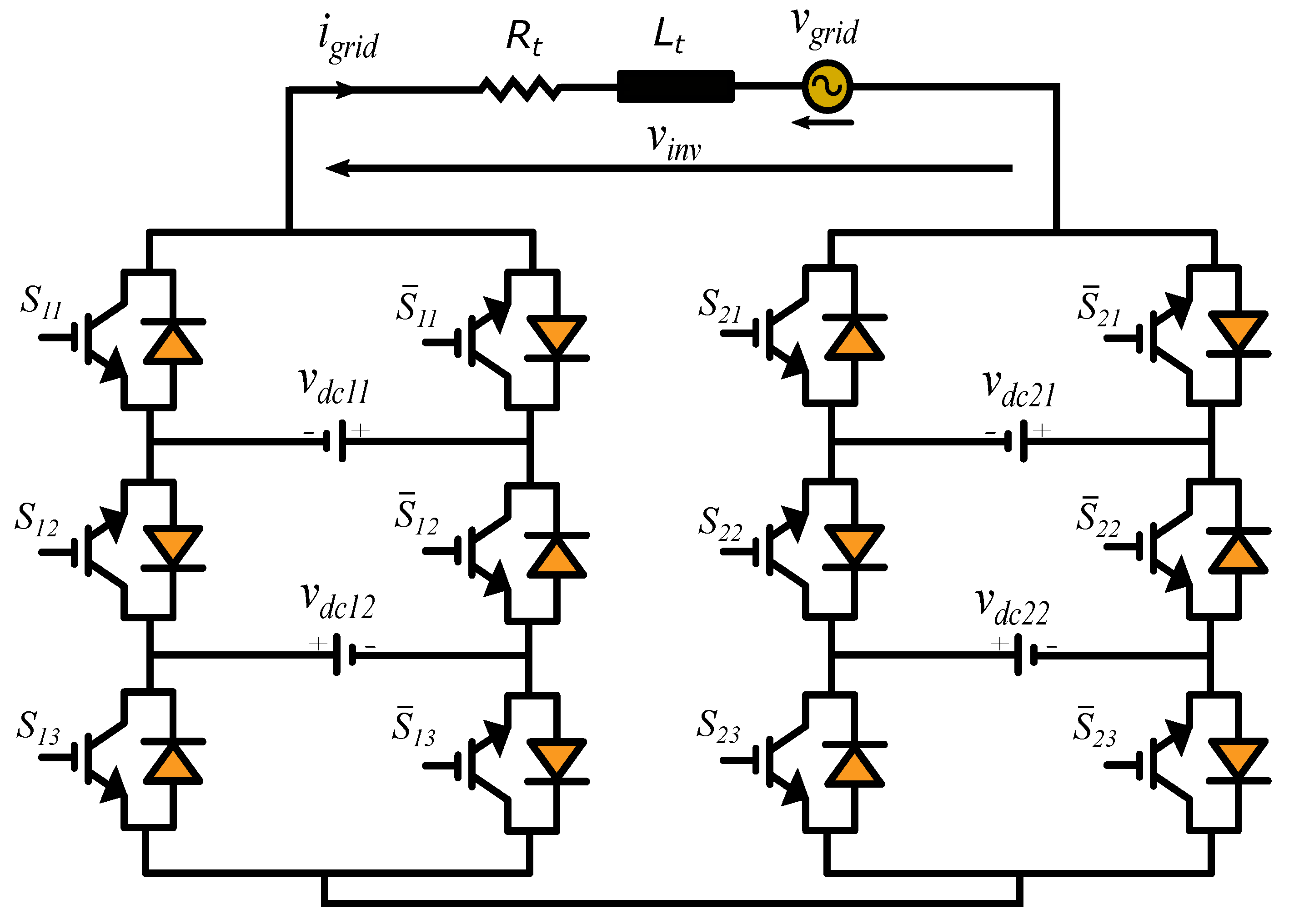
One of the recent competitive topologies of MLIs is the modified packed U-cell MLI (MPUC-MLI) shown in Figure 1. This topology was firstly proposed in [10] as a novel H-bridge unit that is able to generate seven levels by using only six active switches and two isolated DC sources with a binary ratio, whereas the conventional H-bridge unit requires four active switches with a single DC source, producing only three levels in the output voltage. The MPUC-MLI has been proposed to reduce the complexity of the conventional topologies when a large number of levels is required, which makes them impractical. Two cascaded units of this topology, as shown in Figure 1, allow the generation of 49 levels in the output voltage, which results in high power quality with a significant reduction of the filtering requirements [11]. Comprehensive comparisons of this topology with the conventional and recent ones have been conducted in the literature [3,10]. The comparison demonstrates a clear superiority of the MPUC-MLI over the other topologies in terms of the required active switches, power diodes, and drive circuits. Moreover, this topology reduces the voltage blocked by switches, resulting in a low total standing voltage (TSV), which further reduces the size and cost of the converter. Comparing to the packed U-cell MLI (PUC-MLI) [12], the MPUC-MLI has the advantage of boosting capability by adding the two DC links in each unit, which is not achievable in PUC-MLI; on the other hand, isolated DC sources are required for the MPUC-MLI [13]. Based on its features and requirements, the MPUC-MLI is considered most suitable for photovoltaic applications [13]. However, the large number of states results in the complexity of the control for this topology, which is addressed in this work.

Classic control techniques like a PI controller accompanied by a modulation stage and hysteresis nonlinear control are considered the most applied control methods for power converters [14,15,16,17,18]. However, the first method suffers from problematic issues related to parameter tuning and complex implementation, whereas the second has the disadvantage of the variable switching frequency. Additionally, the poor dynamic response is considered a common shortcoming for the traditional control strategies. Consequently, many efforts have recently been focused on adopting advanced control theories for MLI applications to negate these detriments [19,20,21,22]. In addition, the continuous advancement in the field of digital platforms, along with their current huge computational capabilities, has prompted researchers to exploit the merits offered by these advanced technologies [23]. Model predictive control (MPC) is considered one of the most appealing advanced techniques for power electronic converters since it has the ability to take advantage of the discrete nature of power converters. Although MPC applications were limited earlier due to the high computational load, they recently found their way into many applications with the massive development of digital platforms [22,23]. In contrast with traditional control theories, the MPC offers the advantages of nonlinearity inclusion, ease of constraint handling, and superior dynamic response [24]. Based on the way of pulse generation, MPCs can be categorized into two sets: Continuous control set MPCs (CCS-MPCs) and finite control set MPCs (FCS-MPCs). The first category generates a continuous signal for the modulator stage to generate the switching pulses, achieving constant switching frequency, whilst the second exploits the limited switching states of the converter, producing the pulses directly and eliminating the need for any kinds of modulators. Due to the discrete nature of power converters and FCS-MPCs, they have found an attractive common application area [24]. Despite the above-mentioned merits of FCS-MPCs, there are some challenges that need further investigation and effective solutions. Heavy computational load for multilevel and/or multiphase power converters is considered a main issue of FCS-MPCs, which has been addressed in many works; however, it still represents an impediment, particularly for higher-level MLIs [25,26]. Another important concern of FCS-MPCs is the high sensitivity to model parameter variation [27]. A slight change in the parameters’ values may lead to the selection of an incorrect state, which negatively affects the control performance. Therefore, it is unavoidable to consider the parameter variation resulting from some effects, such as thermal effects, aging, and different operation conditions, in order to avoid deterioration of control performance.

1.1. Related Works

FCS-MPCs have been applied for various applications of MLIs with stand-alone and grid-connection modes targeting different control objectives, such as reference current tracking, active and reactive power control, and capacitor voltage regulation [22,28]. A reduced-complexity FSC-MPC for a cascaded H-bridge MLI (CHB-MLI) was proposed in [29]. The idea behind this approach is to calculate the reference voltage vector and then locate the triangular section of this vector. Based on the located section, only three vectors are applied instead of all vectors as in classical FCS-MPC. This strategy has a significant reduction in the number of objective function evaluations; however, further calculations are required to locate the triangular section of the reference vector, particularly for higher-level MLIs, which, in turn, adds more computational load. In [30], a new simplified FCS-MPC is proposed. The idea of this strategy lies in the elimination of the undesirable converter states by using Lyapunov’s theory and the elimination of the weighting factors by employing an optimization method based on fuzzy decision-making. The calculation burden is actually reduced; however, this approach lacks simplicity, which is a distinct feature of FCS-MPCs. In [31], the authors proposed an FCS-MPC for a seven-level PUC-MLI with the objectives of current control at unity power factor and capacitor voltage regulation, employing a weighting factor to handle the two control objectives. The sensitivity to parameter variation was only investigated in this work, without utilizing a method to address this issue. The control of the same topology (PUC-MLI) with FCS-MPC was also designed in [32], who targeted capacitor voltage control and active/reactive power control under different operating conditions. However, neither computational effort reduction nor control sensitivity to model parameters was addressed in this work. An attempt with Lyapunov control theory to simplify the control design of the PUC-MLI by eliminating the gains in the cost function was proposed in [33] with the goal of switching frequency reduction; however, the seven different states of the converter must be evaluated at each sample. Many other strategies are proposed in the literature for various applications with MLI topologies [34,35,36,37]; however, the heavy computational burden and high reliance of the control performance on system model parameters are considered major issues that still need further investigations and improvements.

1.2. Objectives and Contributions

In this paper, two main challenges of FCS-MPCs are addressed for the 49-level MPUC-MLI: the heavy computational load and the MPC’s sensitivity to the variation of the model parameters and measurement noise. The first challenge is addressed by proposing two simplified efficient FCS-MPC approaches inspired by the methods developed in the literature and the proposed concept in [38] for the two-level inverter. The authors refer to the two developed simplified FCS-MPC methods as half-computational-load FCS-MPC (HCL-FCS-MPC) and three-iteration simplified FCS-MPC (TIS-FCS-MPC). Both methods depend on calculating the reference voltage vector from the reference current, exploiting the idea of deadbeat MPCs. Subsequently, based on the voltage vector polarity, the 49 different states of the converter are divided into two sets in the case of the HCL-FCS-MPC; subsequently, the cost function is evaluated only for one set, which results in reducing the computational load. However, in the TIS-FCS-MPC, based on the value of the reference voltage vector, only three states are located and, finally, the cost function is evaluated only three times instead of 49, as in case of conventional FCS-MPC, which results in a significant reduction in the execution time. A mathematical relation is derived to locate the nearest three voltage vectors based on the modified switching table. It is noteworthy that the proposed simplification concept can be applied to different MLI topologies. The second challenge, sensitivity of the control performance to parameter variation and measurement noise, is investigated and tackled in this work by utilizing an extended Kalman filter (EKF) to reinforce the reliability and robustness of the control system. Several simulations studies were carried out using MATLAB/Simulink to validate the proposed concept under different operating conditions.

The contributions of this paper can be summarized as follows:

• Reducing the computational load of the FCS-MPC for higher-level MLI topologies by proposing two efficient and simplified control schemes, which significantly reduce the number of iterations required to achieve grid-current control with switching frequency minimization.
• Investigation of the control’s sensitivity to the system parameters.
• Enhancing the robustness of the FCS-MPC by designing an EKF to estimate the system resistance and inductance online to address the aging and temperature effects.
• Rejection of the measurement noises of the grid current, which is an important concern in real applications.

1.3. Article Organization

The next sections of this paper are organized as follows: Section 2 presents the description and modeling of the competitive 49-level MPUC-MLI. The conventional, HCL-FCS-MPC, and TIS-FCS-MPC algorithms of the considered system are described in Section 3. Section 4 explains the design and implementation of the EKF. Simulation results and discussion are presented in Section 5. Finally, this paper is concluded in Section 6.

2. Description and Modeling of the 49-Level MPUC-MLI

Figure 1 shows the configuration of the considered 49-level MPUC-MLI connected to the grid. The topology under study consists of two units with six active switches and two asymmetric DC sources in each unit. Each unit of this topology produces seven different levels in the output voltage, while two cascaded units with a certain ratio of the DC sources allow the generation of 49 levels. Concerning the count of the used power electronic components and the generated levels, this topology has a considerable reduction in the required components compared to conventional and recent topologies, which results in lower power losses, cost, and installation space. In addition, the generation of such a number of levels is not achievable in most topologies due to the many required components, such as active switches, diodes, and capacitors, which make these topologies impractical for higher levels. However, some applications have been reported in the literature for MLIs with a large number of output levels to improve the power quality. In [11], the implementation of two cascaded PUC-MLIs producing 49 levels in the output voltage with variable frequency control is presented. The application of an 81-level hybrid MLI for an induction motor drive with zero common-mode voltage is proposed in [39]. Thanks to the large number of levels generated, high-quality waveforms are obtained, which reduce the filter requirements and further reduce the system’s cost. Based on the features and requirements, most of the recently developed MLIs are considered application-oriented topologies [40]. Accordingly, the aforementioned merits of this topology and the requirements, which are mainly the required isolated DC sources, make this topology most suitable for photovoltaic (PV) applications by providing the required DC sources from PV arrays (the PV application is not addressed in this work).

Referring to Figure 1, switches $S_{ij}$ and ${\overline{S}}_{ij}$ are switched in a complementary way, where $i\in \{1,2\}$ is the unit number and $j\in \{1,2,3\}$ is the cell number in the unit. Ideal switches are considered; hence, the state of $S_{ij}$ is defined as

$$S_{ij}=\{\begin{array}{c}1,\mathrm{for}\mathrm{ON}-\mathrm{state}\hfill \\ 0,\mathrm{for}\mathrm{OFF}-\mathrm{state}.\hfill \end{array}$$

(1)

The output voltage vector produced by the inverter can be expressed as

$$v_{inv}=(S_{12}-S_{11})V_{dc11}+(S_{12}-S_{13})V_{dc12}+(S_{22}-S_{21})V_{dc21}+(S_{22}-S_{23})V_{dc22},$$

(2)

where $V_{dc11}$, $V_{dc12}$, $V_{dc21}$, and $V_{dc22}$ are the values of the DC sources. To generate the maximum number of levels from this topology, the DC source values are determined by

$$V_{dcij}=2^{j-1}{7}^{i-1}{V}_s,$$

(3)

where $V_s$ is the value of the level step. Based on the number of cells included (six cells), the considered MPUC-MLI has 64 states $\left(2^6\right)$, which are 49 different vectors and 15 redundant states (

Table 1. Switching table of the 49-level MPUC-MLI.

${\mathit{S}}_{11}$	${\mathit{S}}_{12}$	${\mathit{S}}_{13}$	${\mathit{S}}_{21}$	${\mathit{S}}_{22}$	${\mathit{S}}_{23}$	${\mathit{u}}_{\mathit{i}\mathit{n}\mathit{v}}$	State
1	0	1	1	0	1	−24	1
0	0	1	1	0	1	−23	2
1	0	0	1	0	1	−22	3
0	0	0	1	0	1	−21	4
1	1	1	1	0	1	−21	5
0	1	1	1	0	1	−20	6
..	..	..	..	..	..	..	..
0	0	0	0	0	0	0	31
0	0	0	1	1	1	0	32
1	1	1	1	1	1	0	33
1	1	1	0	0	0	0	34
..	..	..	..	..	..	..	..
1	0	0	0	1	0	20	59
0	0	0	0	1	0	21	60
1	1	1	0	1	0	21	61
0	1	1	0	1	0	22	62
1	1	0	0	1	0	23	63
0	1	0	0	1	0	24	64

). Taking $V_s$ as a base value, $u_{inv}$ is defined as the per-unit output inverter voltage, where $u_{inv}=v_{inv}/V_s$ and $u_{inv}\in \{-24,23,\dots ,23,24\}$. The redundancy is only provided for the vectors that have zero-voltage generated by the first and/or second unit. Typically, the redundant states of such converters are exploited for switching frequency reduction and/or capacitor voltage regulation [41]. However, from the viewpoint of control complexity, the redundant states increase the computation effort. For the considered topology, no capacitors are included, and a low switching frequency is also achieved without using the redundant states, as illustrated in the simulation results (Section 5). Consequently, to simplify the control design, only the different vectors (49 vectors) are considered in the control design. In doing so, new variables, $S1$ to $S4$, are used and can be defined as

$$\begin{array}{c}{S}_1=S_{12}-S_{11},\\ S_2=S_{12}-S_{13},\\ S_3=S_{22}-S_{21},\\ S_4=S_{22}-S_{23}.\end{array}$$

(4)

Table 2. Modified switching table of the 49-level MPUC-MLI.

${\mathit{S}}_1$	${\mathit{S}}_2$	${\mathit{S}}_3$	${\mathit{S}}_4$	${\mathit{u}}_{\mathit{i}\mathit{n}\mathit{v}}$	State$\mathit{N}$
−1	−1	−1	−1	−24	1
0	−1	−1	−1	−23	2
−1	0	−1	−1	−22	3
0	0	−1	−1	−21	4
1	0	−1	−1	−20	5
..	..	..	..	..	..
0	0	0	0	0	25
..	..	..	..	..	..
−1	0	1	1	20	45
0	0	1	1	21	46
1	0	1	1	22	47
0	1	1	1	23	48
1	1	1	1	24	49

lists the possible different switching states of the considered 49-level MPUC-MLI using the new variables, $S_1$ to $S_4$. Note that N represents the state number of the MPUC-MLI in Table 2, $N\in \{1,2,\dots ,49\}$. Hence, the generated voltage vector from this topology can be rewritten as

$$v_{inv}=S_1{V}_{dc11}+S_2{V}_{dc12}+S_3{V}_{dc21}+S_4{V}_{dc22}.$$

(5)

By applying Kirchhoff’s voltage law, the voltage equation at the grid side of the MLI system shown in Figure 1 is expressed as

$$v_{inv}=R_t{i}_{grid}+L_t\frac{d{i}_{grid}}{dt}+v_{grid},$$

(6)

where $R_t$ and $L_t$ are the total resistance and inductance of the system, respectively, i.e., filter and grid parameters. $v_{grid}$ and $i_{grid}$ are the grid voltage and current, respectively.

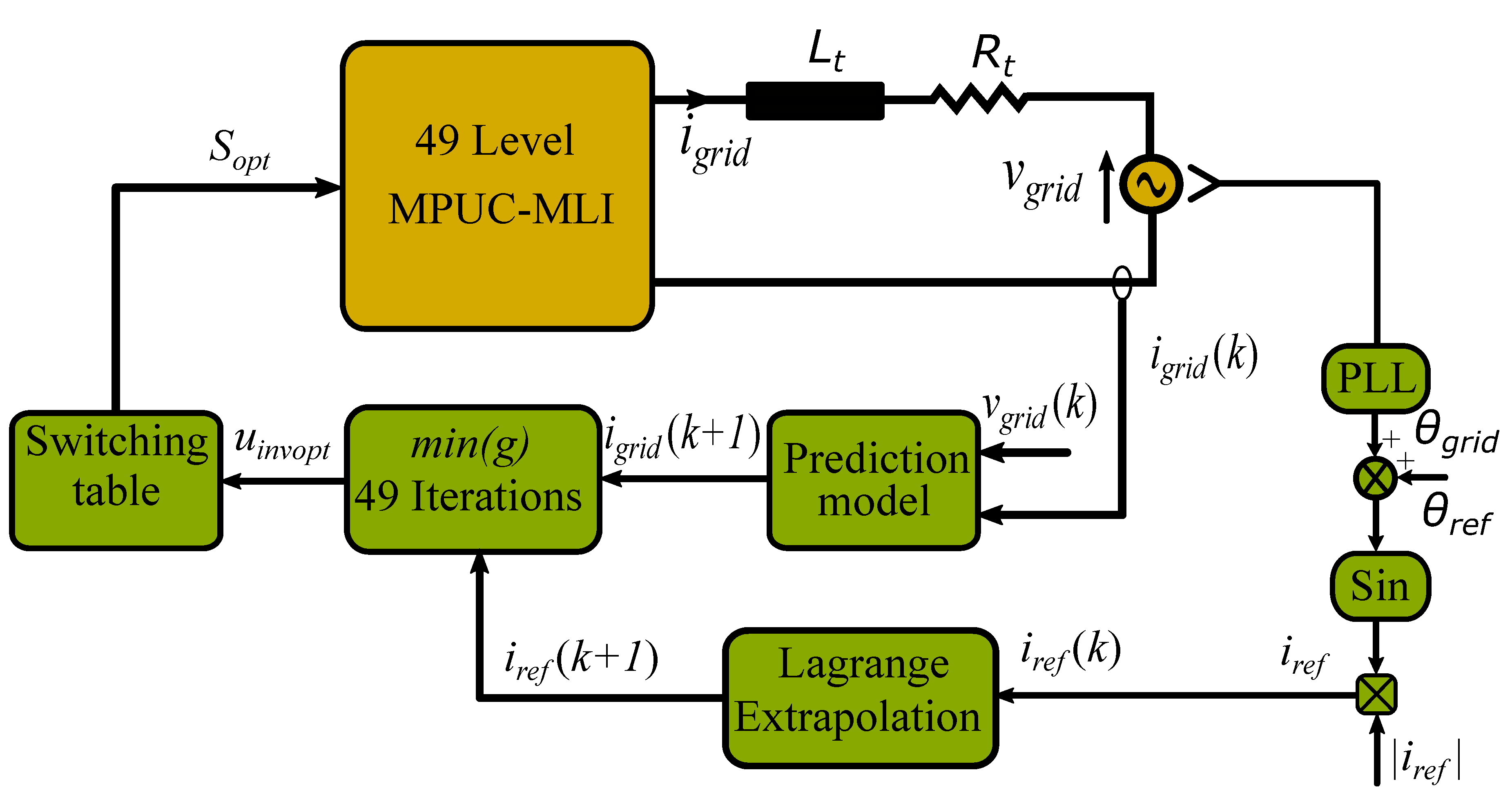
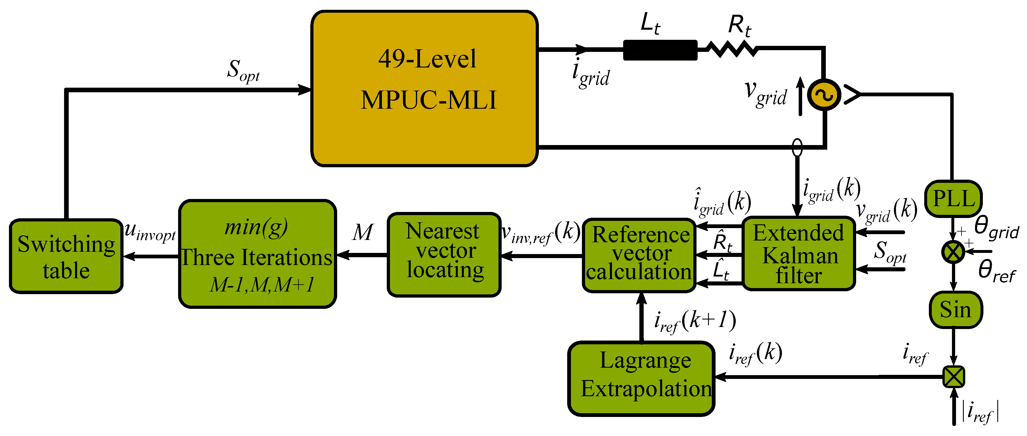
3. Control of the 49-Level MPUC-MLI

Conventional FCS-MPC has been implemented for many MLI topologies [22,24,28]; however, the heavy computational load remains a major disadvantage, especially for higher-level converters because, in this technique, the prediction of the controlled variables and the cost function minimization should be calculated for each state of the converter per iteration. Thus, much effort has been focused on developing simplified schemes of the FCS-MPC that reduce the number of calculations without deteriorating control performance [29,30,31,32]. In this work, a 49-level MLI is considered to address this issue. In the following subsections, the conventional strategy and the two proposed simplified FCS-MPC strategies are described for the considered MPUC-MLI. The prediction model, cost function design, and optimization algorithm are explained for the three methods. The cost function is designed with two control objectives: reference current tracking and switching frequency minimization. The reference current angle is produced depending on the grid angle generated by a conventional phase-locked loop (PLL) and the added angle ${\theta }_{ref}$, which represents the targeted phase shift between the grid voltage and current in order to allow different power factor (PF) operations, whereas the reference current amplitude is determined based on the required amount of injected power (see Figure 2).

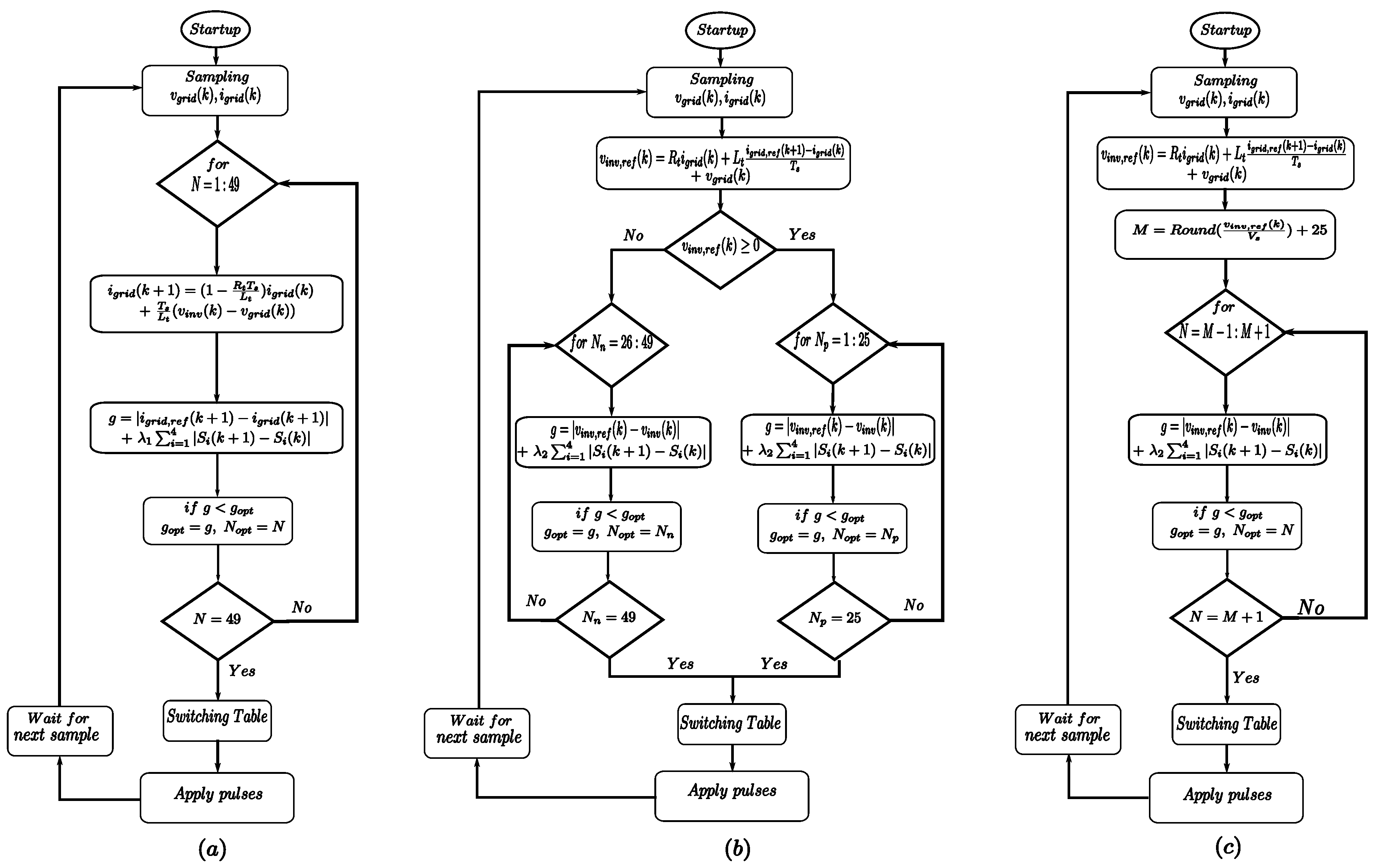
3.1. Conventional FCS-MPC

Figure 2 depicts the schematic diagram of the conventional FCS-MPC for the grid-connected MPUC-MLI. The discrete-time model of the system is considered the main core of the FCS-MPC, as it is required to predict the controlled variables. To discretize the system model, various discretization techniques exist, such as the Euler method and Taylor series expansion [42,43]. In this work, Euler forward approximation is considered. Referring to Equation (6), applying Euler forward approximation, and solving for $i_{grid}(k+1)$ yields

$$i_{grid}(k+1)=(1-\frac{R_t{T}_s}{L_t})i_{grid}\left(k\right)+\frac{T_s}{L_t}(v_{inv}\left(k\right)-v_{grid}\left(k\right)),$$

(7)

where $i_{grid}\left(k\right)$ and $i_{grid}(k+1)$ are the the grid current at present sampling instant $\left(k\right)$ and the next one $(k+1)$, respectively. $T_s$ denotes the sampling time. Based on the control objectives, the cost function is expressed as

$$g=|i_{grid,ref}(k+1)-i_{grid}(k+1)|+{\lambda }_1\sum _{i=1}^4|S_i(k+1)-S_i\left(k\right)|,$$

(8)

where $i_{grid,ref}(k+1)$ is the reference current value at the next sample, and ${\lambda }_1$ is the weighting factor used to handle the priority of the two objectives. $S_i\left(k\right)$ and $S_i(k+1)$ denote the states of $S_i$ at instants k and $k+1$. By employing the Lagrange extrapolation method, $i_{grid,ref}(k+1)$ is estimated as

$$i_{grid,ref}(k+1)=3i_{grid,ref}\left(k\right)-3i_{grid,ref}(k-1)+i_{grid,ref}(k-2).$$

(9)

In this method and based on the basic idea of the FCS-MPC, the grid current prediction and the cost function are computed for all different voltage states (49 states, see Table 2) in order to identify the optimal voltage vector $u_{invopt}$, whose cost function is minimal; finally, the switching table is utilized to generate the pulses to the switches based on $u_{invopt}$.

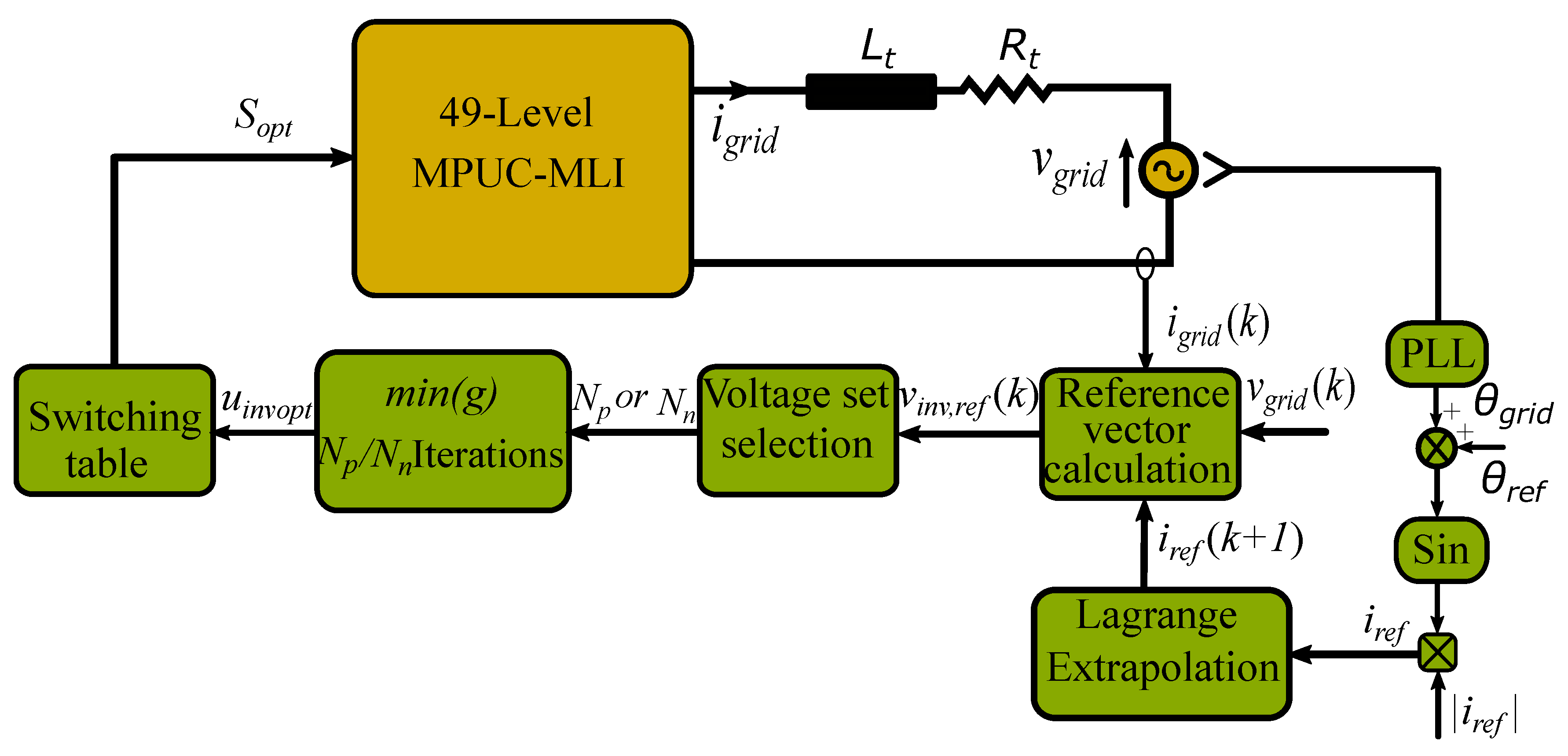
3.2. Half-Computational-Load FCS-MPC

For the conventional FCS-MPC, 49 iterations are required for grid current prediction and cost function calculations for each sample, which, in turn, represent a high computational load. As a result, a long time is required for the algorithm execution, which negatively affects the control performance and could be an obstacle to the experimental implementation. Therefore, the need to reduce the execution time of the considered MLI is inevitable.

The prime control goal of the MPUC-MLI under study is to identify the converter state that makes the predicted current $i_{grid}(k+1)$ follow its reference $i_{grid,ref}(k+1)$. In doing so, $i_{grid}(k+1)$ is replaced with $i_{grid,ref}(k+1)$ in Equation (7). Accordingly, the inverter output voltage $v_{inv}\left(k\right)$ can be considered as the reference inverter voltage $v_{inv,ref}\left(k\right)$, whose tracking error is minimal. Doing so and solving Equation (7) for $v_{inv,ref}\left(k\right)$ yields

$$v_{inv,ref}\left(k\right)=R_t{i}_{grid}\left(k\right)+L_t\frac{i_{grid,ref}(k+1)-i_{grid}\left(k\right)}{T_s}+v_{grid}\left(k\right).$$

(10)

Noticing Table 2, one can conclude that based on the polarity of $u_{inv}$, two sets can be identified for N: $N_p\in \{1,2,\dots ,25\}$ for non-negative values of $u_{inv}$ and $N_n\in \{26,27,\dots ,49\}$ for negative values of $u_{inv}$. The inverter output voltage can be expressed as

$$v_{inv}\left(k\right)=\{\begin{array}{c}{u}_{inv}\left(N_p\right)V_s,N_p\in \{1,2,\dots 25\},\mathrm{if}{v}_{inv,ref}\left(k\right)\ge 0\hfill \\ u_{inv}\left(N_n\right)V_s,N_n\in \{26,27,\dots 49\},\mathrm{if}{v}_{inv,ref}\left(k\right)<0.\hfill \end{array}$$

(11)

Subsequently, the cost function is designed as

$$g=|v_{inv,ref}\left(k\right)-v_{inv}\left(k\right)|+{\lambda }_2\sum _{i=1}^4|S_i(k+1)-S_i\left(k\right)|.$$

(12)

Accordingly, compared to the conventional FCS-MPC, the number of cost function calculations per sample has almost halved. Moreover, no current predictions are required. As a result, the computational burden has been considerably reduced. The detailed block diagram of the HCL-FCS-MPC is shown in Figure 3.

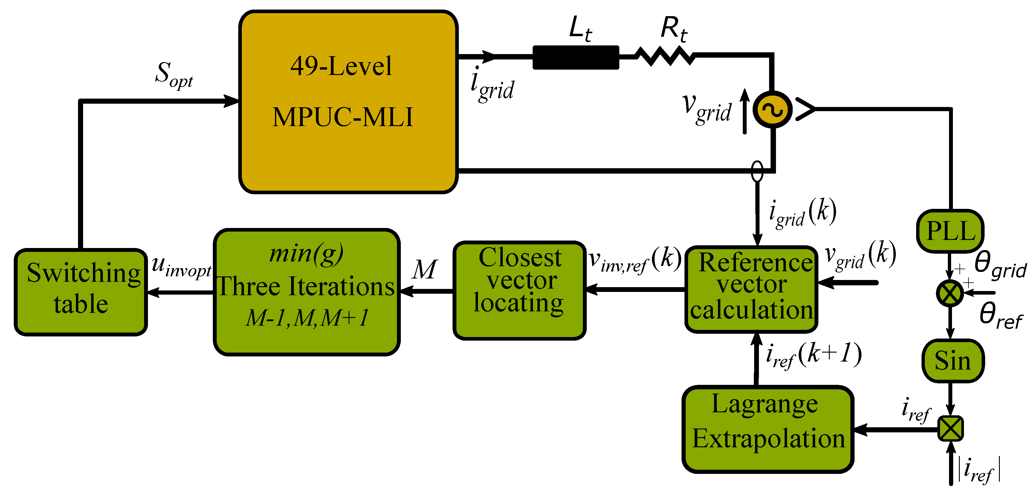
3.3. Three-Iteration Simplified FCS-MPC

In this method, further simplification is achieved by locating a narrower section of the voltage vectors to be considered for the cost function minimization. The idea of this approach lies in exploiting the relation between the generated voltage vectors of the MPUC-MLI and the state number. With a closer look at Table 2, one can find a relation between the per-unit voltage vector and the state number, $u_{inv}$ and N. It is worth mentioning that the switching table has been rearranged to find such a relation. From Table 2, it can be concluded that the equation $N=u_{inv}+25$ applies to all MPUC-MLI states. This means that once the reference voltage vector is determined, the nearest corresponding state can be identified. For more accuracy and tolerance to achieve other control objectives, the three closest states are employed to minimize the cost function. Thus, the authors call this method the three-iteration simplified FCS-MPC (TIS-FCS-MPC). The detailed block diagram of this scheme is depicted in Figure 4. After calculating the reference voltage vector using Equation (10), a new variable M is defined as

$$M=Round(\frac{v_{inv,ref}\left(k\right)}{V_s})+25.$$

(13)

Then, the three selected states for cost function minimization are $M-1$, M, and $M+1$. Note that the utilized cost function is the same as in the HCL-FCS-MPC method (Equation (12)).

Accordingly, 49 iterations of the current prediction are saved, and only three cost function calculations are computed per sample in the proposed TIS-FCS-MPC method. As a result, compared to the previous two control methods, this algorithm has a minimum computational burden and execution time. The flowcharts of the three applied control schemes are shown in Figure 5.

4. Extended Kalman Filter Design for the Grid-Connected 49-Level MPUC-MLI

The extended Kalman filter has been widely adopted in many applications in different fields due to its abilities of parameter estimation and noise rejection [44]. The EKF is considered the modified approach of the Kalman filter for nonlinear systems and its design mainly depends on the discrete-time nonlinear model of the system [45].

Since the FCS-MPC’s performance is highly dependent on the accuracy of the system modeling, it is necessary to consider the variation of the parameters due to thermal effects, aging, and/or different operating conditions in order to avoid the degradation of the control performance. A slight variation in the parameters’ values could lead to an incorrect selection of the converter state, which adversely impacts the stability or deteriorates the control response. Additionally, the proposed simplification concept is based on the reference voltage calculation according to Equation (10) to minimize the cost function in Equation (12). From Equation (10), one can observe that the accuracy of the reference voltage depends on the accuracy of the system resistance and inductance. However, in the conventional method, the reference current is directly employed in the cost function, as shown in Equation (8). Therefore, to consider this issue in the proposed concept and ensure accurate values of system parameters, the EKF is adopted as an online estimator. The parameters of the filter and grid are estimated online in order to eliminate the reliance of the FCS-MPC on the system parameters and to reinforce the system robustness. In addition, the grid current is estimated to reject the measurement noise, which is actually an important concern. The block diagram of the proposed TIS-FCS-MPC with the implemented EKF for the grid-connected MPUC-MLI is shown in Figure 6.

To design the EKF, the nonlinear discrete model of the considered system is required in the state-space form. In doing this, Equation (6) is solved for $d{i}_{grid}/dt$, which results in

$$\frac{d{i}_{grid}}{dt}=-\frac{R_t}{L_t}{i}_{grid}+\frac{1}{L_t}(v_{inv}-v_{grid}).$$

(14)

The state-space model of the 49-level grid-connected MPUC-MLI including disturbances can be expressed as

$$\begin{array}{c}\dot{x}=\mathbf{A}x+\mathbf{B}u+w,\hfill \\ y=\mathbf{C}x+\mathbf{D}u+v,\hfill \end{array}$$

(15)

where x, u, and y are the state vector, input, and output of the system, respectively. $\mathbf{A}$, $\mathbf{B}$, $\mathbf{C}$, and $\mathbf{D}$ are the system matrices, which represent the parameters of the system. w and v represent the incertitude and measurement noise of the system, respectively. Q and R are the covariance matrices of w and v, respectively. Since the covariance matrices have a significant effect on the estimation process, particle swarm optimization (PSO) is used to determine their entry values [46]. Based on the considered grid-connected MPUC-MLI system, referring to Equation (14), the following matrices can be defined as

$$x=\left[\begin{array}{c}{i}_{grid}\\ R_t\\ L_t\end{array}\right],u=[\begin{array}{c}{v}_{inv}-v_{grid}\end{array}],y=[\begin{array}{c}{i}_{grid}\end{array}],\mathbf{A}=\left[\begin{array}{ccc}-\frac{R_t}{L_t}& 0& 0\\ 0& 0& 0\\ 0& 0& 0\end{array}\right],\mathbf{B}=\left[\begin{array}{c}\frac{1}{L_t}\\ 0\\ 0\end{array}\right],\mathbf{C}=[\begin{array}{ccc}1& 0& 0\end{array}],\mathbf{D}=0.$$

(16)

Subsequently, by applying forward Euler approximation to Equation (15), the discrete-time model of the system can be written as

$$\begin{array}{c}x(k+1)={\mathbf{A}}_{d}x\left(k\right)+{\mathbf{B}}_{d}u\left(k\right)+w\left(k\right),\hfill \\ y\left(k\right)={\mathbf{C}}_{d}x\left(k\right)+{\mathbf{D}}_{d}u\left(k\right)+v\left(k\right),\hfill \end{array}$$

(17)

where the matrices ${\mathbf{A}}_{\mathbf{d}}$, ${\mathbf{B}}_{\mathbf{d}}$, ${\mathbf{C}}_{\mathbf{d}}$, and ${\mathbf{D}}_{\mathbf{d}}$ can be defined as

$${\mathbf{A}}_{\mathbf{d}}=\left[\begin{array}{ccc}1-\frac{T_s{R}_t}{L_t}& 0& 0\\ 0& 1& 0\\ 0& 0& 1\end{array}\right],{\mathbf{B}}_{\mathbf{d}}=\left[\begin{array}{c}\frac{T_s}{L_t}\\ 0\\ 0\end{array}\right],{\mathbf{C}}_{\mathbf{d}}=[\begin{array}{ccc}1& 0& 0\end{array}],{\mathbf{D}}_{\mathbf{d}}=0.$$

(18)

Actually, the system incertitude and measurement noise are not known; thus, the EKF is used as follows,

$$\begin{array}{c}\widehat{x}(k+1)={\mathbf{A}}_d\widehat{x}\left(k\right)+{\mathbf{B}}_{d}u\left(k\right)+\mathbf{K}\left(k\right)(y\left(k\right)-\widehat{y}\left(k\right)),\hfill \\ \widehat{y}\left(k\right)={\mathbf{C}}_d\widehat{x}\left(k\right)+{\mathbf{D}}_{d}u\left(k\right),\hfill \end{array}$$

(19)

where $\mathbf{K}\left(k\right)$ represents the Kalman gain, and $\widehat{x}\left(k\right)$ and $\widehat{y}\left(k\right)$ are the estimated values of the state variable and system output, respectively. The implementation of the EKF algorithm can be mainly summarized in two phases—prediction and correction.

The prediction phase includes the state vector prediction according to Equation (19) and the prediction of covariance matrix error as

$${\mathbf{P}}^{-}\left(k\right)=f\left(k\right)\mathbf{P}(k-1)f{\left(k\right)}^{\mathrm{T}}+\mathbf{Q},$$

(20)

where

$$f\left(k\right)=\frac{\partial }{\partial x}{({\mathbf{A}}_{d}x\left(k\right)+{\mathbf{B}}_{d}u\left(k\right))}_{{\widehat{x}}^{-}\left(k\right)}.$$

(21)

The correction phase of the state vector and covariance matrix error is carried out as

$$\mathbf{K}\left(k\right)={\mathbf{P}}^{-}\left(k\right){\mathbf{C}}_d^{\mathrm{T}}{({\mathbf{C}}_d{\mathbf{P}}^{-}\left(k\right){\mathbf{C}}_d^{\mathrm{T}}+\mathbf{R})}^{-1},$$

(22)

$$\widehat{x}\left(k\right)={\widehat{x}}^{-}\left(k\right)+\mathbf{K}\left(k\right)(y\left(k\right)-{\mathbf{C}}_d{\widehat{x}}^{-}\left(k\right)),$$

(23)

$$\mathbf{P}\left(k\right)={\mathbf{P}}^{-}\left(k\right)-\mathbf{K}\left(k\right){\mathbf{C}}_d{\mathbf{P}}^{-}\left(k\right).$$

(24)

5. Results and Discussion

In this section, simulation studies are carried out using MATLAB/Simulink to validate the proposed concepts. Firstly, the conventional technique and the two proposed FCS-MPC techniques for the grid-connected 49-level MPUC-MLI are simulated and compared, taking into account different performance indicators in different operating conditions. After validation of the proposed FCS-MPC methods, the TIS-FCS-MPC is considered for the next investigations due to its superior performance and lower computational burden compared to the other two schemes, as illustrated in the next subsection. At this point, the weighting factor ${\lambda }_2$ is tuned and switching frequency minimization is considered as a second control objective. The sensitivity of the proposed TIS-FCS-MPC is investigated with respect to the model parameters to illustrate the effect of parameter mismatch on control performance, and finally, the proposed EKF is implemented to address this concern. Several results are obtained for the proposed EKF with the considered grid-connected system.

The simulation parameters of the considered system are listed in

Table 3. Grid-connected 49-level MPUC-MLI parameters.

Parameter	Value
Grid voltage $v_{grid}$ ($\mathrm{V}$)	220
Grid frequency $\omega$ ($\mathrm{rad}/\mathrm{s}$)	$2\pi \times 50$
Total resistance (filter and grid) $R_t$ ($\Omega$)	$0.2$
Total inductance (filter and grid) $L_t$ ($\mathrm{m}\mathrm{H}$)	10
Level step value $v_s$ ($\mathrm{V}$)	15
Sampling time $T_s$ [$\mathsf{\mu }\mathrm{s}$]	100

. Note that the values of the DC sources are determined based on Equation (3) to maximize the amount of output voltage generated by the MPUC-MLI with 49 levels. It is worth mentioning that unity power factor operation is considered for the results; however, the system has the ability to inject current into the grid at different power factors, as previously discussed.

5.1. Reference Current Tracking

The simulation models of the three control algorithms are built based on Figure 2, Figure 3 and Figure 4 with the objective of grid current reference tracking (i.e., ${\lambda }_1$ and ${\lambda }_2$ are set to zero). The performance indicators used to visualize the comparisons between the three methods are the mean absolute tracking error $e_i$ expressed as a percentage of reference current amplitude [22], average switching frequency $f_s$, total harmonic distortion of the inverter output voltage $\left(TH{D}_{vinv}\right)$, and execution time of the algorithm. $f_s$ of the considered MPUC-MLI can be expressed as

$$f_s=\frac{{\sum }_{i=1}^2{\sum }_{j=1}^3{f}_{ij}}{6}.$$

(25)

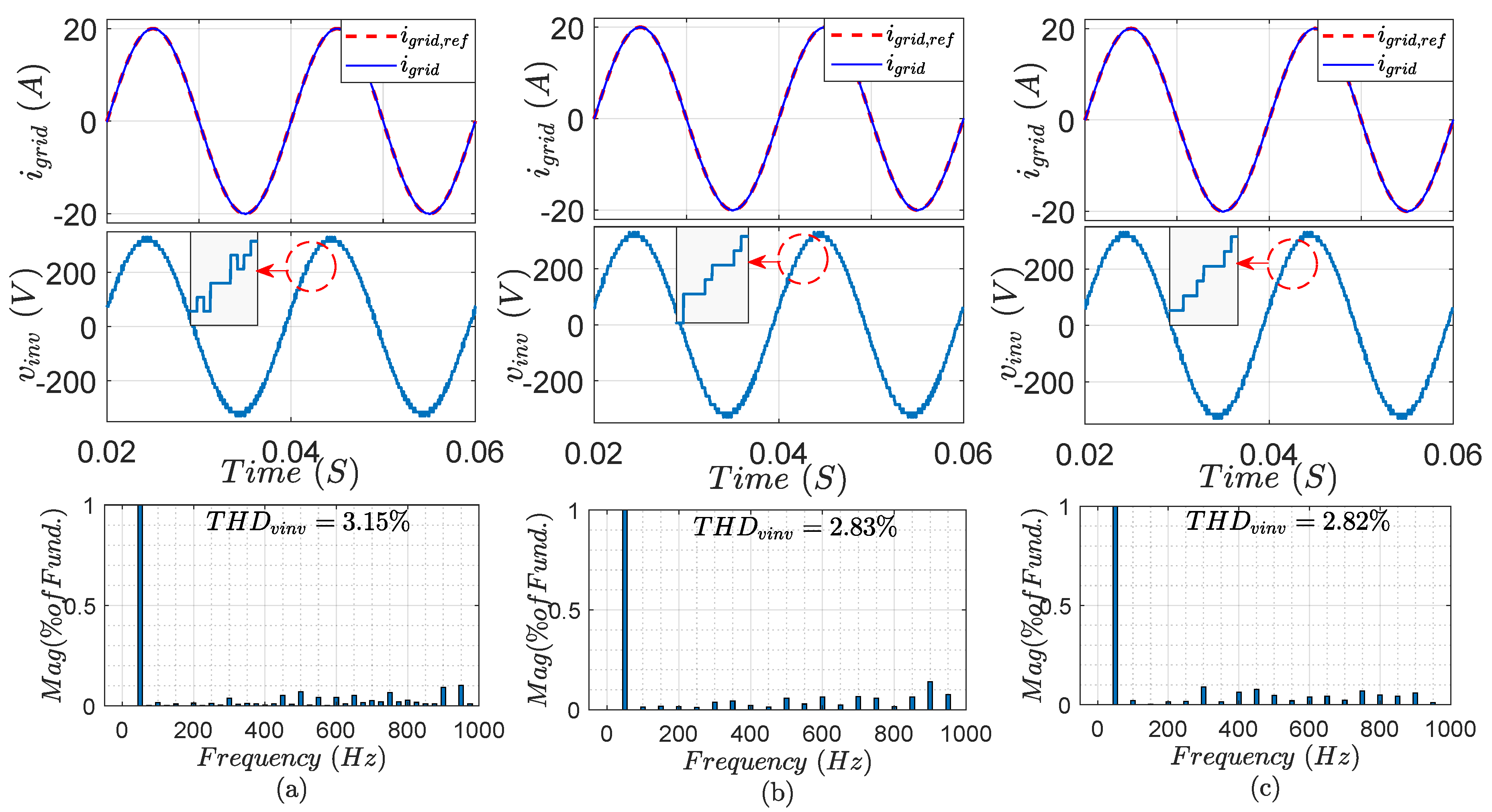
Figure 7 shows the injected grid current, inverter output voltage, and the inverter voltage spectrum for the conventional, HCL-FCS-MPC, and TIS-FCS-MPC schemes. From the figure, it is clear that the three control methods have a perfect current tracking capability and nearly sinusoidal output voltage with very low $TH{D}_{vinv}$. The harmonic spectrum across the frequency, as well as the THD, meet the standard requirements for grid-connected systems [47].

The tracking quality of the current control is evaluated in this work by considering $e_i$ as a performance indicator. For the conventional, HCL-FCS-MPC, and TIS-FCS-MPC algorithms, $e_i$ was found to be very low: $0.3\%$, $0.23\%$, and $0.2\%$, respectively, while $f_s$ was recorded at 960, 945, and 885 Hz, respectively. Moreover, the proposed TIS-FCS-MPC has a minimum execution time of $9\mathsf{\mu }\mathrm{s}$ compared to the other two methods, while the HCL-FCS-MPC and the conventional FCS-MPC schemes require execution times of 35 and $51\mathsf{\mu }\mathrm{s}$, respectively, which means a reduction of $31\%$ and $82\%$ has been achieved in the execution time for the proposed HCL-FCS-MPC and TIS-FCS-MPC compared to the conventional FCS-MPC. To visualize the comparisons between the three control algorithms, the considered performance indicators in the steady-state operation are listed in

Table 4. Steady-state comparative results of the three FCS-MPC schemes.

Parameter	Conventional FCS-MPC	HCL-FCS-MPC	TIS-FCS-MPC
Execution time [$\mathsf{\mu }\mathrm{s}$]	51	35	9
$e_i$	$0.3\%$	$0.23\%$	$0.2\%$
$f_s$ [Hz]	960	945	885
$TH{D}_{vinv}$	$3.15\%$	$2.83\%$	$2.82\%$

.

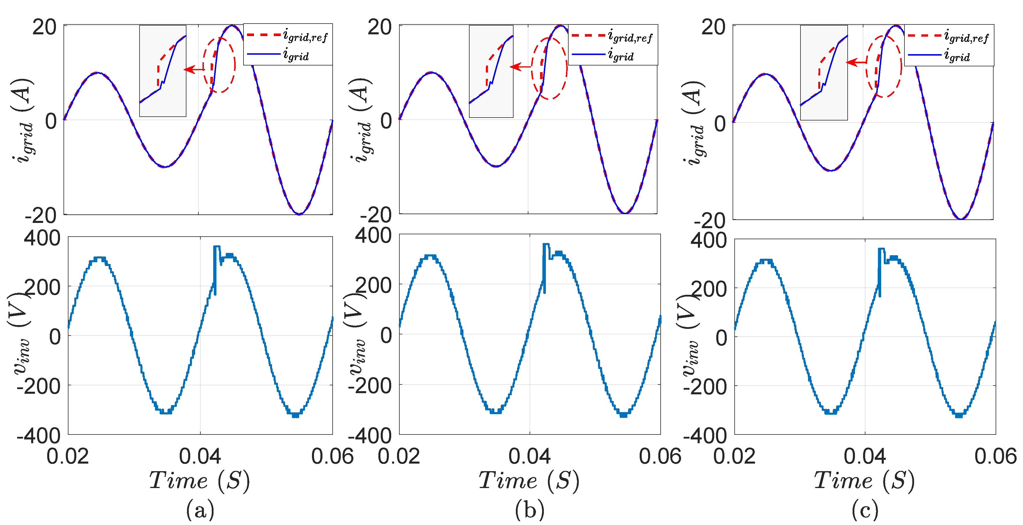
To investigate the dynamic response, a step-change in the reference grid current from 10 to 20 A was made, as shown in Figure 8. As shown in the results for the three control algorithms, the grid current is perfectly following its reference, achieving very low transient time.

From the results, one can conclude that the proposed simplified algorithms select the optimal voltage vector, as in the conventional method; moreover, better performance indicators for the simplified methods are recorded, as they have lower execution times thanks to the reduced computational load, which is consistent with the theoretical analysis.

5.2. Switching Frequency Minimization

Since the proposed TIS-FCS-MPC method has superior performance and minimum execution time compared to the other algorithms, it will be considered for the following investigations. To evaluate the control system with the two objectives, as in Equation (12), ${\lambda }_2$ is first tuned to achieve the desired performance, and then the results are obtained.

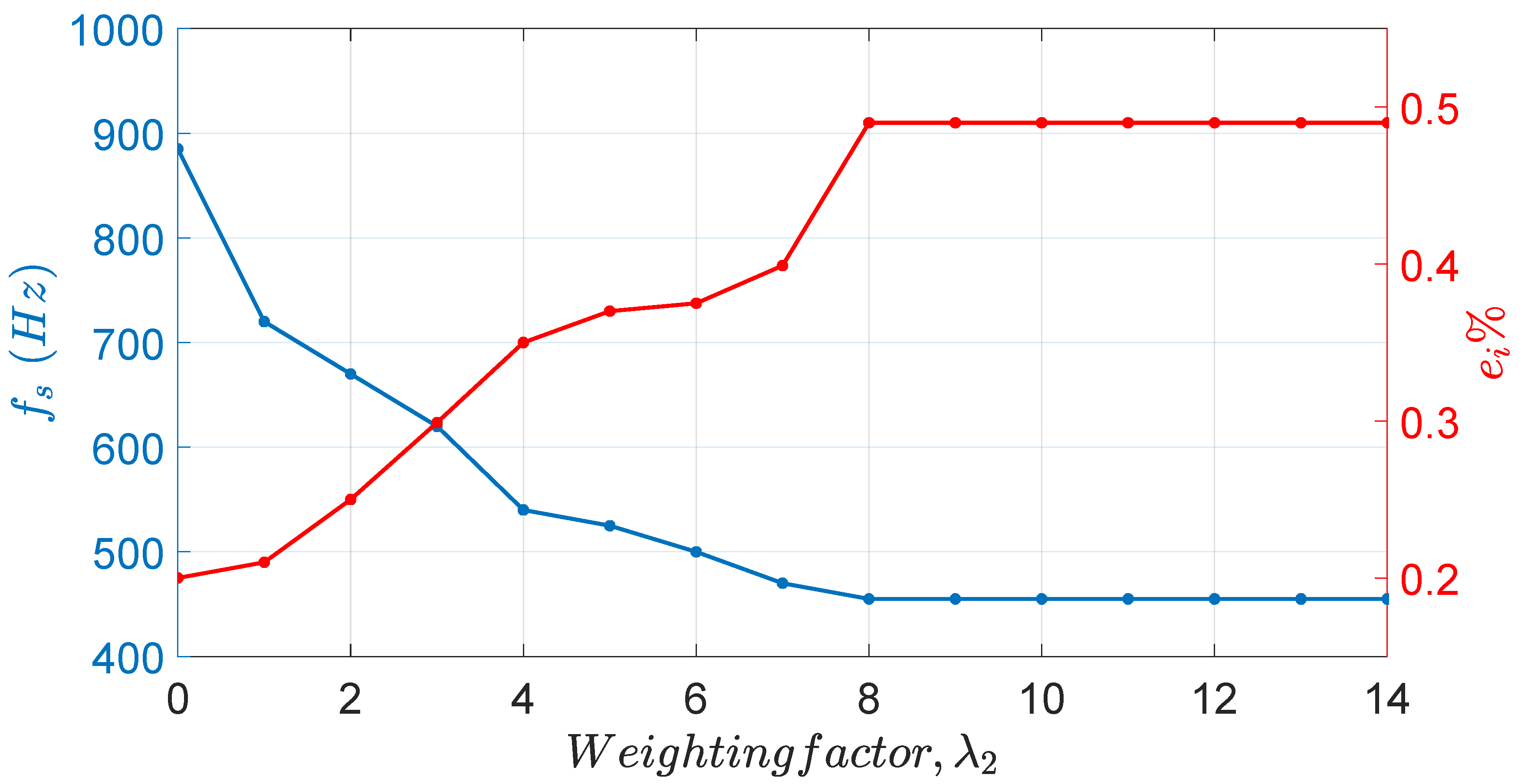
5.2.1. Weighting Factor Tuning

The tuning of ${\lambda }_2$ is carried out considering the desired performance of the tracking quality and switching frequency. To clarify the effect of ${\lambda }_2$ on the control performance, $e_i$ and $f_s$ are taken as evaluation parameters and measured for different values of ${\lambda }_2$. Figure 9 depicts the values of $e_i$ and $f_s$ through a wide range of ${\lambda }_2$. As noticed in the figure, for ${\lambda }_2=0$ to ${\lambda }_2=8$, $e_i$ increases from $0.2\%$ to $0.49\%$, whereas $f_s$ decreases from 885 to 455 Hz. Beyond that (i.e., ${\lambda }_2>8$), $e_i$ and $f_s$ were found to be constant. The reason behind this lies in the low number of voltage vectors under selection. As discussed earlier, only the three closest vectors are used for the cost function minimization, ensuring good tracking quality with a limited value of $e_i$ regardless of the selected vector. Hence, for ${\lambda }_2\ge 8$, high tracking quality $(e_i=0.49\%)$ and minimum switching frequency $(f_s=455\mathrm{Hz})$ can be achieved. By setting ${\lambda }_2\gg 8$, no further tuning is required for different operating conditions, which is considered another important feature of the proposed TIS-FCS-MPC. Accordingly, the value of ${\lambda }_2$ of 8 is set as optimal in the next investigations.

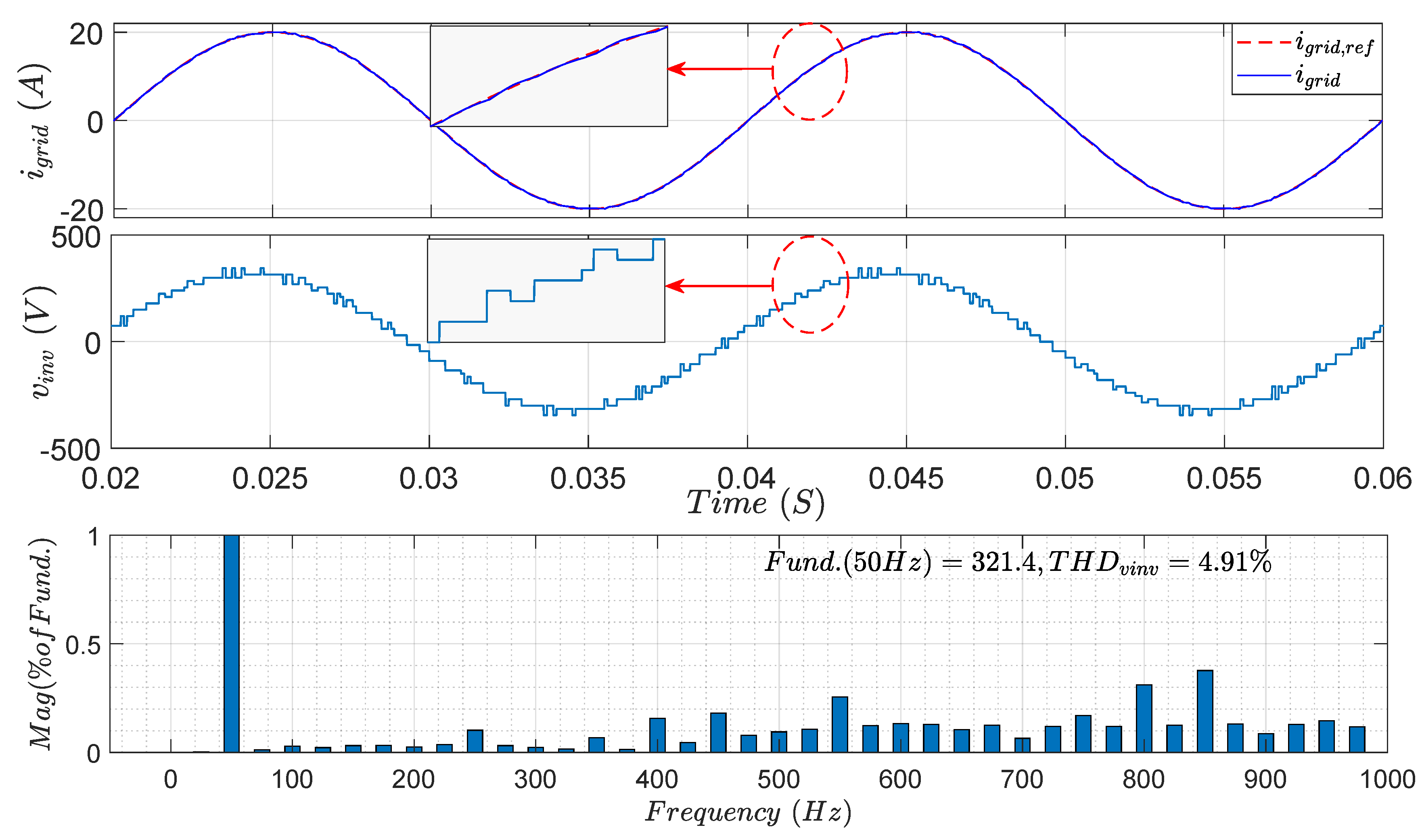
5.2.2. Simulation Results at ${\lambda }_{2opt}$

The simulation results of the TIS-FCS-MPC for the grid-connected system under control with the two targeted control objectives at ${\lambda }_2=8$ are shown in Figure 10. Comparing to the results at ${\lambda }_2=0$ (see Figure 7c and Table 4), a slight increase in $e_i$ was recorded (from $0.2\%$ to $0.49\%$) and a significant decrease in $f_s$ was achieved (from 885 to 455 Hz). However, $TH{D}_{vinv}$ has increased from $2.82\%$ to $4.91\%$. From the results, it can be concluded that switching frequency minimization with high tracking and waveform quality can be achieved at ${\lambda }_2\ge 8$.

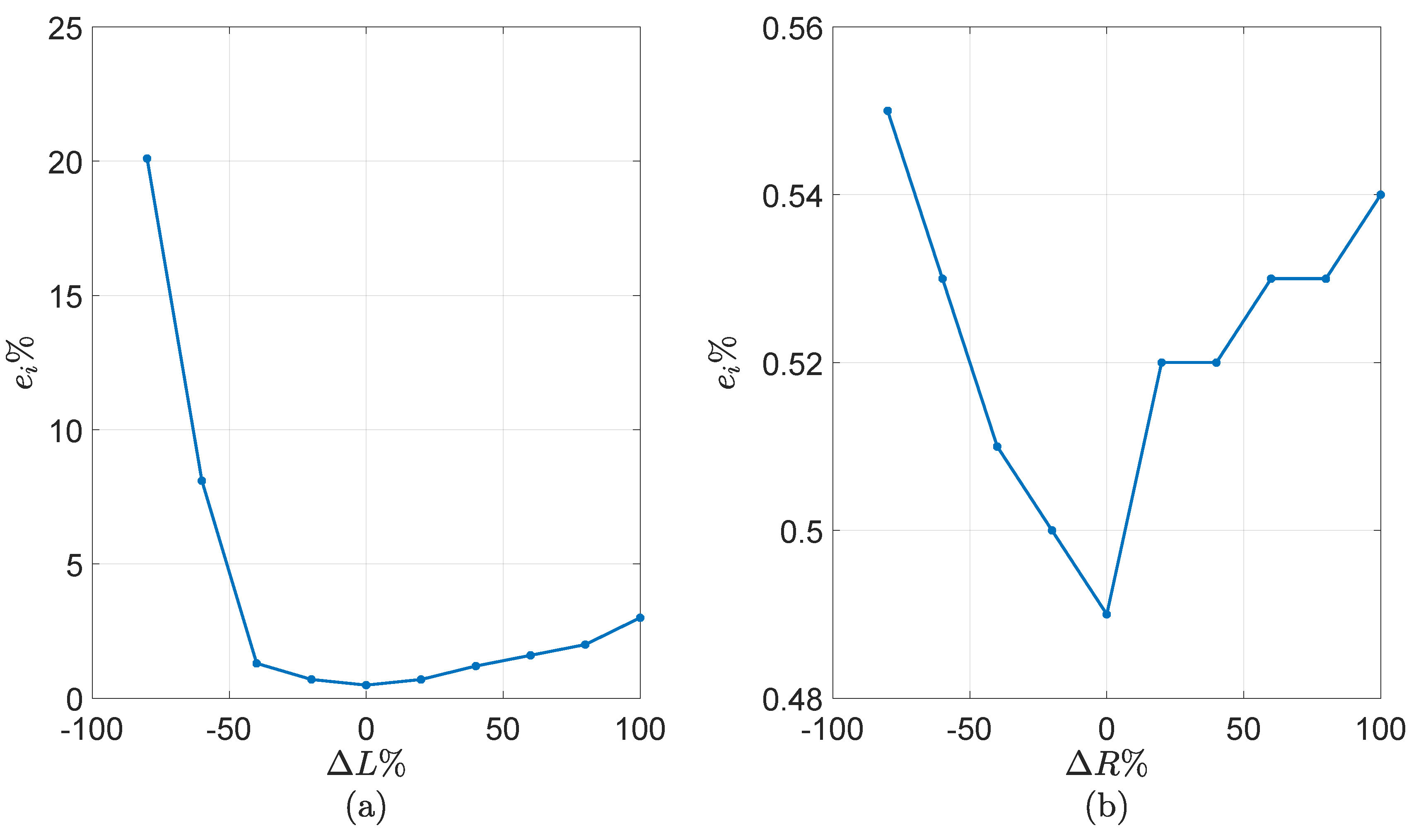
5.3. Control Sensitivity to System Parameter Variations

The sensitivity of the proposed TIS-FCS-MPC to parameter variations is investigated by changing the system parameters and monitoring the control performance. The parameters considered in the analysis are $L_t$ (total inductance of the grid and filter) and $R_t$ (total resistance of the grid and filter), while $e_i$ is monitored as the performance indicator. Ten measured points are recorded through a specified range of variation, $-80\%$ to $100\%$. To decouple the effect of each parameter, only one parameter is changed at a time. The simulation results of this analysis are shown in Figure 11. It can be seen that the control performance is more sensitive for the system inductance. An $-80\%$ change in $L_t$ increases $e_i$ significantly from $0.49\%$ to $20\%$. On the other side, the variation of $R_t$ has less impact on $e_i$, as shown in the figure. For a $50\%$ change in $R_t$, $e_i$ has an increase of only approximately $0.15\%$.

From the sensitivity analysis, it is clear that the issue of the FCS-MPC’s reliance on parameter variation should be considered, especially for inductance variation.

5.4. Simulation Results for the Proposed EKF

The complete model of the considered grid-connected system is simulated in this subsection by adopting the proposed TIS-FCS-MPC with the designed EKF, as shown in Figure 6. Note that ${\lambda }_2$ is set to its optimal value (${\lambda }_{2opt}=8$). System parameter variations ($R_t$ and $L_t$) and measurement noises of the grid current are handled by the implemented EKF. The simulation parameters are the same as those listed in Table 3 except for $T_s$, which is reduced to $40\mathsf{\mu }\mathrm{s}$ to obtain a better response from the EKF.

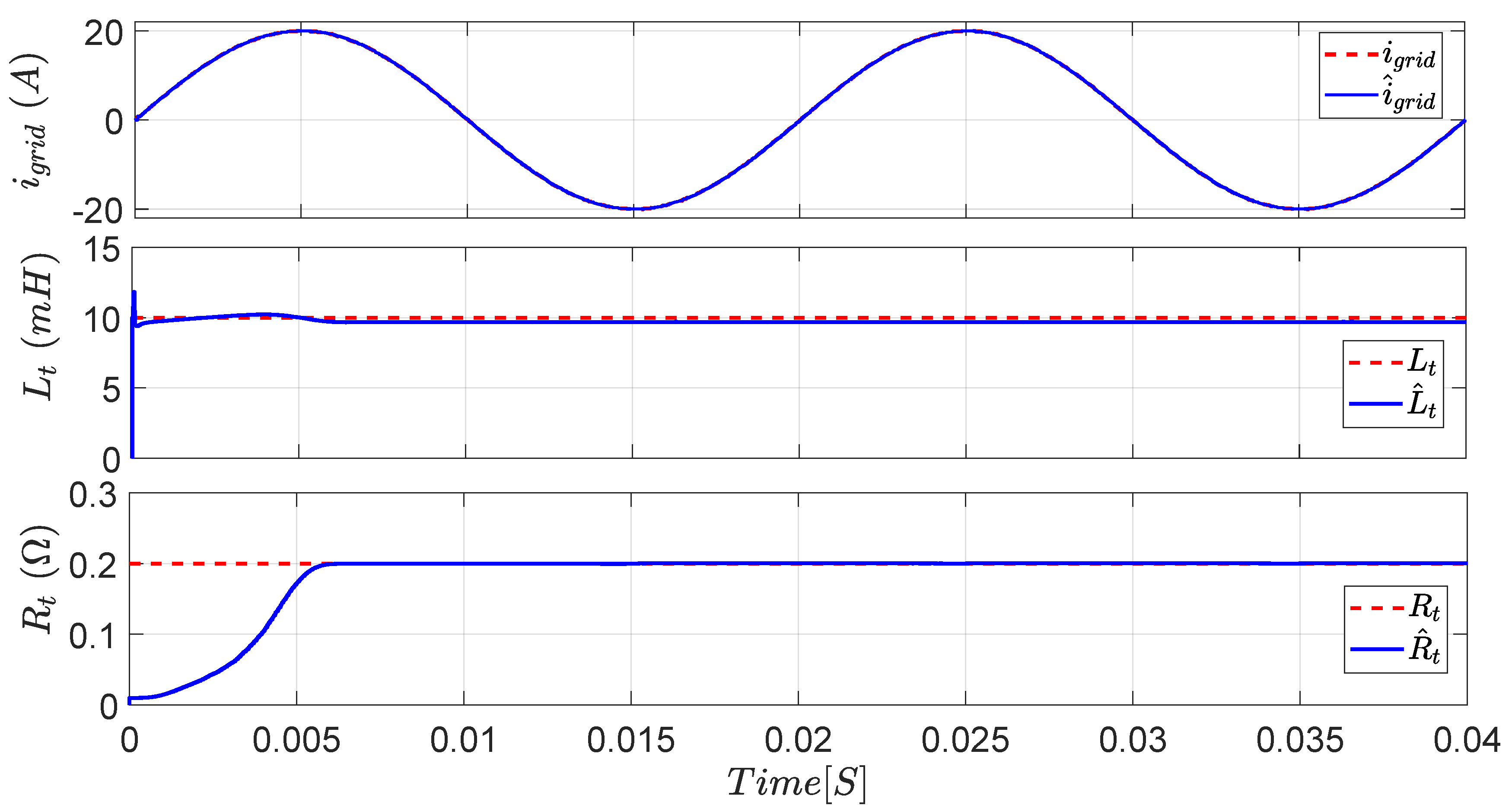
Figure 12 shows the results of the designed EKF for the estimations of the grid current ${\widehat{i}}_{grid}$, system inductance ${\widehat{L}}_t$, and resistance ${\widehat{R}}_t$. The EKF provides an efficient and accurate estimation capability. The actual and estimated grid currents are nearly identical. The estimation process of the system inductance exhibits a very fast and accurate response with a steady-state error $e_{ss}$ of $1.5\%$, whereas, for the system resistance, the estimation is comparatively slower, with a very low $e_{ss}$ of $0.4\%$.

Figure 13 depicts the EKF’s performance for a step-change in the grid current. The current is stepped down at $t=0.041S$ from 20 to 10 A and then stepped up at $t=0.082S$ to 30 A. The results show an excellent estimation of the grid current in all cases. However, $e_{ss}$ of ${\widehat{L}}_t$ has a slight increase with decreasing grid current. A small disturbance is observed at the stepping instants of the current for ${\widehat{R}}_t$; however, $e_{ss}$ is still very low.

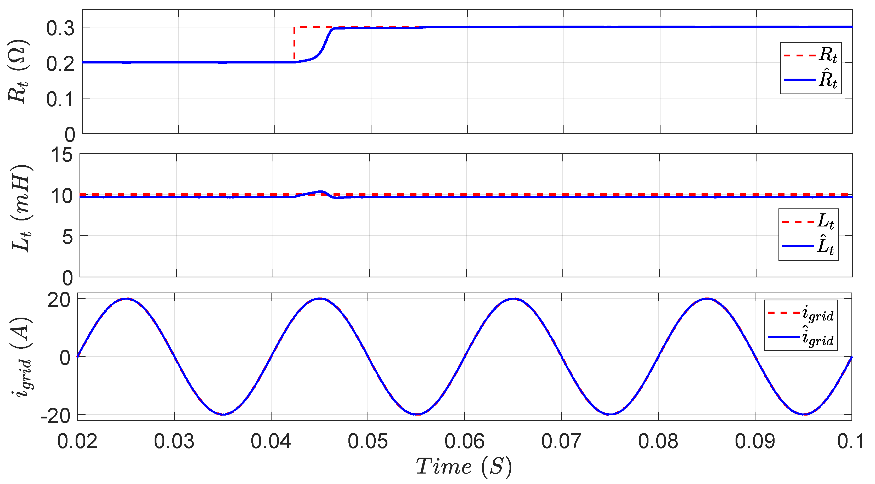
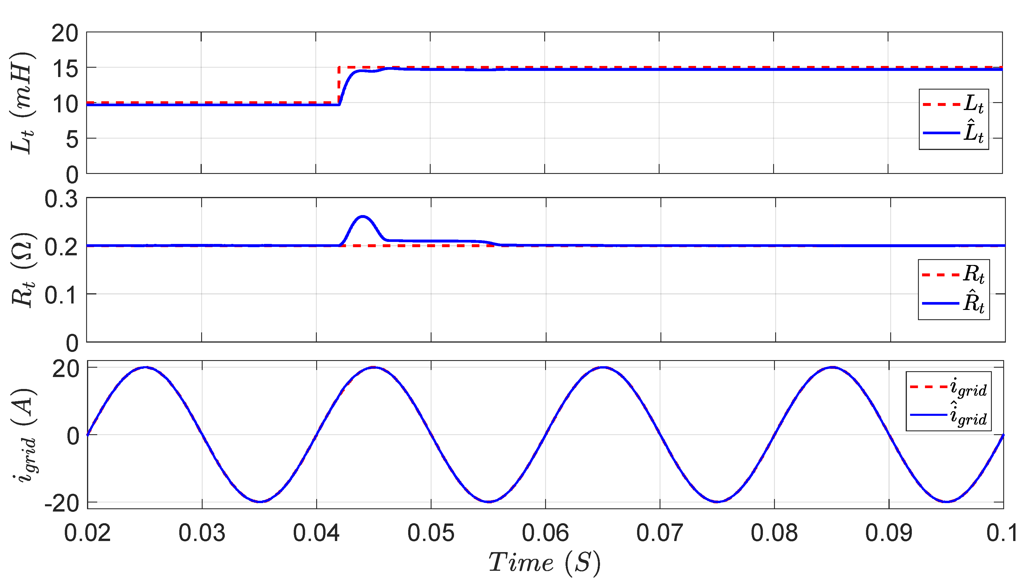
Figure 14 and Figure 15 illustrate the EKF’s response for a step-change in $L_t$ and $R_t$, respectively. $L_t$ is increased by $50\%$, from its nominal value of 10 to 15 mH. It is obvious from Figure 14 that ${\widehat{L}}_t$ follows $L_t$ with a very fast response. A $25\%$ overshoot is observed in ${\widehat{R}}_t$ for a short period, but quickly returns to its actual value. In Figure 15, $R_t$ is increased from $0.2$ to $0.3\mathsf{\Omega }$, showing high estimation quality for ${\widehat{R}}_t$. From these investigations, it is clear that the proposed EKF design has the ability to accurately estimate the system parameters and the actual grid current with a fast dynamic response under different disturbances.

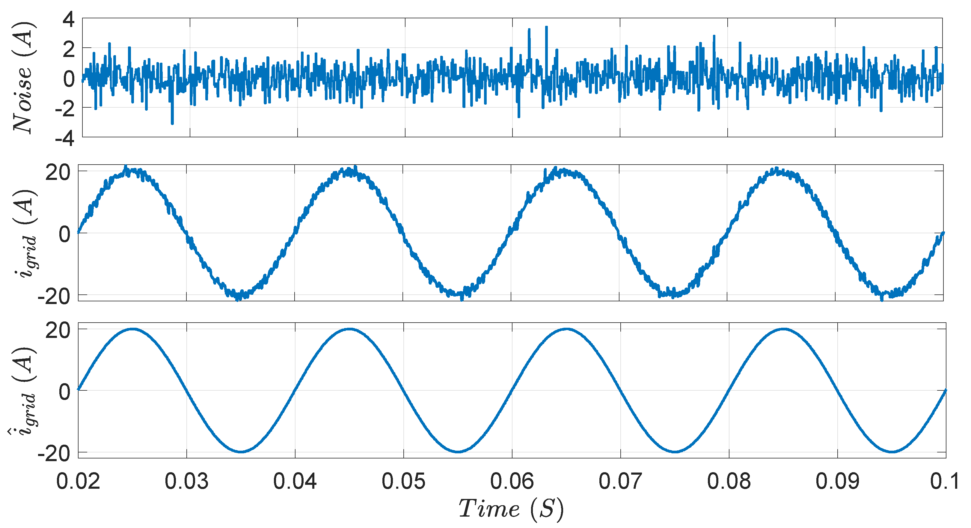
The EKF’s capability to filter the grid current from the measurement noise is also investigated. To assess the filtering ability of the EKF, white noise is added to the actual grid current, and then the noisy current is inputted to the EKF. Figure 16 shows the added noise, noisy grid current, and the estimated current. The estimated grid current has much lower noise content, proving the EKF’s noise filtering efficacy.

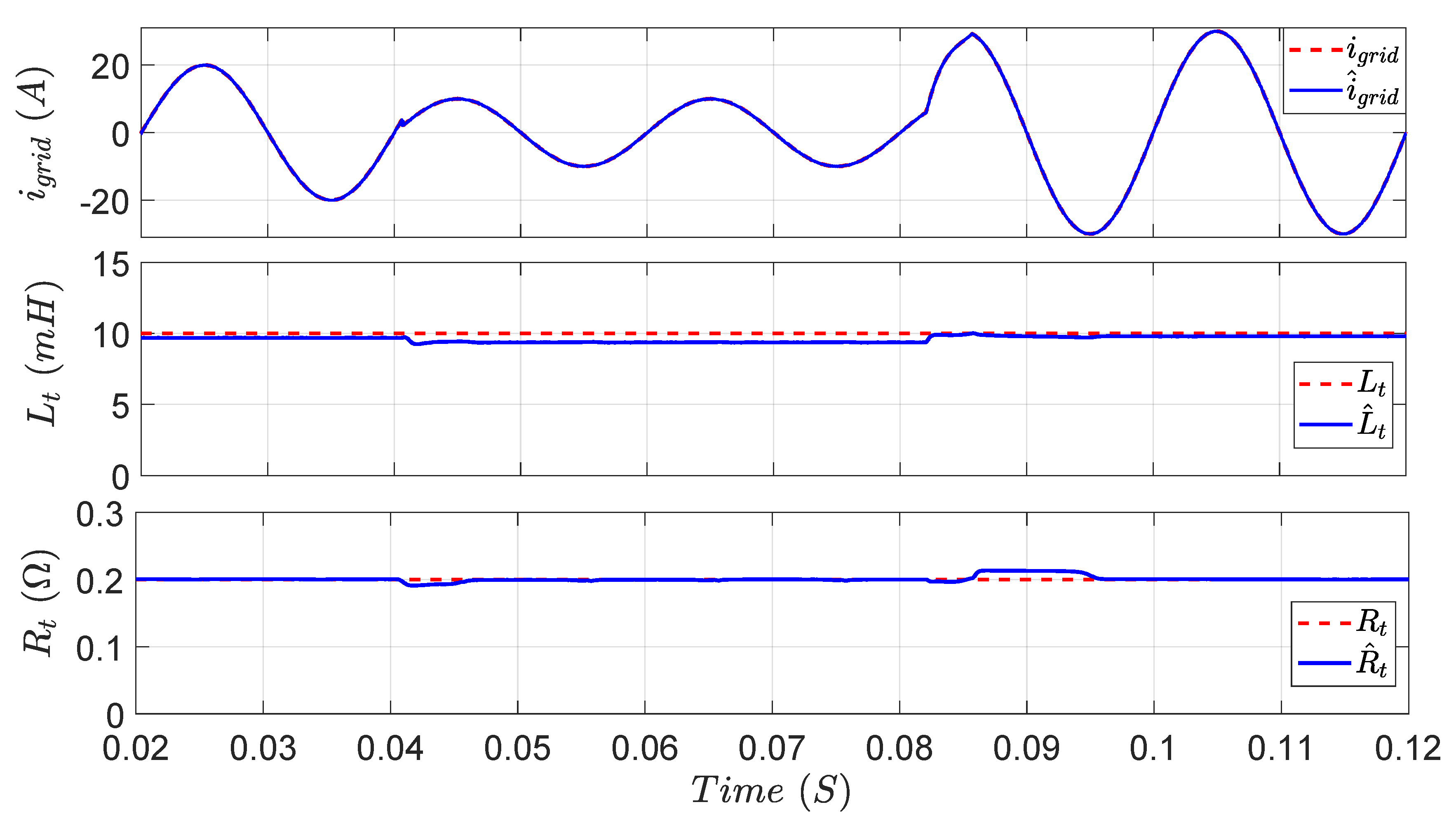
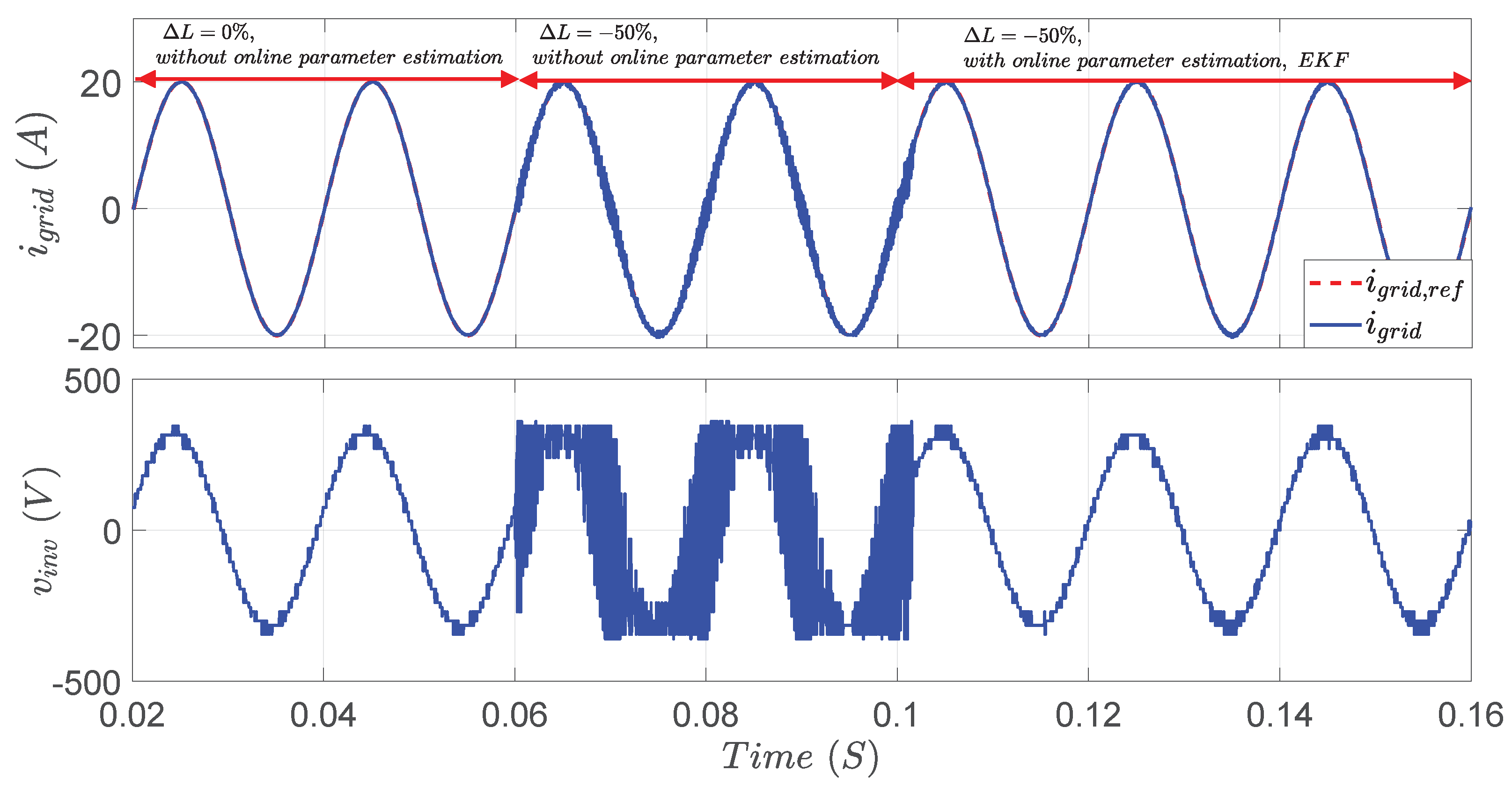
Finally, to demonstrate the significance of the EKF in the considered system, the output inverter voltage $v_{inv}$ and grid current $i_{grid}$ are monitored under three different conditions, as depicted in Figure 17. During the first two cycles, the system works at the nominal parameters’ values without online parameter estimation, exhibiting good control performance. Suddenly ($t=0.06S$), $L_t$ is decreased by $50\%$ without employing the EKF. As a result, distorted grid current with high $e_i$ is observed. Additionally, highly distorted voltage with considerable harmonic contents is noticed. After two cycles ($t=0.1S$), the EKF is activated and, hence, the system parameters are estimated online. As shown in the figure, the grid current returns to its sinusoidal form with low $e_i$, achieving high tracking quality. In addition, the inverter voltage is significantly improved with respect to the harmonic contents.

6. Conclusions

In this article, the heavy computational load of the FCS-MPC for high-level MLIs has been addressed. The proposed simplification concept has been applied to a grid-connected cascaded MPUC-MLI system. Two efficient simplified FCS-MPC schemes have been proposed, namely a half-computational-load FCS-MPC (HCL-FCS-MPC) and a three-iteration simplified FCS-MPC (TIS-FCS-MPC). The proposed methods have been compared with the conventional one. The comparison has proved the effectiveness of the considered solutions. The execution time has been reduced by $31\%$ and $82\%$ for the HCL-FCS-MPC and TIS-FCS-MPC, respectively, compared to the conventional one. Moreover, better performance has been achieved for the TIS-FCS-MPC concerning $e_i$ and $f_s$. Switching frequency minimization has been targeted as a second objective in the cost function after tuning ${\lambda }_2$. As a result, a $50\%$ reduction of $f_s$ has been realized. At ${\lambda }_2\gg 8$, the proposed TIS-FCS-MPC allows operation at different conditions without the need to retune ${\lambda }_2$. Sensitivity analysis of the system has been conducted and showed a high dependency on system inductance. To enhance the system’s immunity to parameter mismatch and robustness against disturbances, an EKF was designed to estimate system parameters and filter the noise of measurements. The proposed EKF has achieved high reliability and robustness of the system under large variations in parameters as well as with measurement noise. The high estimation accuracy and filtering potential of the proposed EKF were validated through the simulation results. Although the proposed FCS-MPC schemes achieved a significant reduction in the computational burden with a superior control performance for a grid-connected system, the variable switching frequency is still considered a major challenge that should be addressed in future works.