Abstract
Integrated biomass gasification combined cycles can be advantageous for providing multiple products simultaneously. A new electricity and freshwater generation system is proposed based on the integrated gasification and gas turbine cycle as the main system, and a steam Rankine cycle and multi-effect desalination system as the waste heat recovery units. To evaluate the performance of the system, energy, exergy, and economic analyses were performed. Also, a parametric analysis was performed to assess the effects of various parameters on the system’s performance criteria. The economic feasibility of the plant was analyzed in terms of net present value. For the base case, the performance metrics are evaluated as , , , and . Among all components of the system, the combustion chamber is the greatest contributor to the exergy destruction rate, at 3250 kW. It is shown with the parametric analysis that raising the combustion temperature leads to higher electricity and freshwater production capacity. For a fuel cost of and an electricity price of , the total net present value at the end of plant’s lifespan is , and the payback period is years. Thus, the plant is feasible from an economic perspective.
1. Introduction
Renewable energy resources such as biofuels are receiving significant attention worldwide. Being available extensively and replenishable, biomass and wastes from various resources such as residues of agricultural, forestry, dairy, and domestic activities can be regarded as sustainable resources []. Moreover, biomass and various wastes can be employed to drive several systems for such products as electricity, heat, cooling, potable water, ethanol, and renewable biodiesel, via various conversion pathways [].
Among the conversion pathways, gasification is an efficient method for syngas production. Gasification of biomass and wastes includes partial oxidation in a closed chamber to yield gaseous products []. Among the different types of gasification, the fixed-bed downdraft gasifier is recognized by many as advantageous since it has a relatively high conversion efficiency compared to other gasification methods [].
The final syngas produced is usually used in subsequent conversion processes, including combustion in a gas turbine. The concept of integration of the gasification process with a gas turbine cycle for electricity generation was introduced by Weil [] in 1950. The integrated gasification combined cycle (IGCC) combines a solid fuel gasification unit with an integrated gas turbine-steam power plant to enhance performance and achieve higher efficiency []. To enhance the power generation capacity, the off-gases of the gas turbine are used as an energy source to drive a steam cycle through a heat recovery steam generator (HRSG) []. For instance, Soltani et al. [] analyzed an integrated biomass gasification and gas turbine combined cycle from energy and exergy perspectives. They indicated that, for a particular gas turbine inlet temperature and cold-end temperature difference of the heat exchanger, the thermal efficiency of the system could be maximized by adjusting pressure ratio. Gholamian et al. [] proposed a novel multi-generation system based on an IGCC, which includes a biomass gasification system, a gas turbine cycle, a supercritical CO2 cycle, and a domestic water heater. For the case of wood as the biomass input, the highest exergy efficiency was calculated to be 40.1%. Ahmadi et al. [] applied a steam Rankine cycle (SRC) to recover the waste energy of a micro gas turbine and analyzed the system from thermodynamic, environmental, and exergoeconomic viewpoints. They also carried out optimization and employed evolutionary algorithms to determine the optimum design parameters. Köse et al. [] investigated the utilization of the steam Rankine cycle and organic Rankine cycle (ORC) as the bottoming cycle of the gas turbine. They performed a parametric optimization to analyze the effects of the various working fluids in the ORC subsystem. The optimum performance criteria are obtained for the overall system, including the SRC–ORC bottoming cycle with R141b as the working fluid. Optimal values of the first-law efficiency, the second-law efficiency, and the net output power were evaluated as 22.6%, 64.8%, and 780 kW, respectively.
Waste energy recovery in cement processing has been studied by Wang et al. [], in terms of four bottoming systems: single-flash and dual-pressure steam systems, a Kalina cycle (KC) and an ORC. The highest efficiency was obtained for the Kalina cycle. A Kalina cycle was combined with a Brayton Rankine cycle by Singh and Kaushik [] to enhance the first- and second-law efficiencies and to decrease CO2 emissions. Considering a constant fuel use, the energy and exergy efficiencies for this novel hybrid system are increased by about 0.54% and 0.51%, respectively, relative to the base system. Cao et al. [] provided a parametric study and optimization for a biomass-driven Kalina cycle in the presence and absence of a regenerative heater. They found that the efficiency of the cycle is enhanced by using the regenerative heater.
Freshwater shortages are significant concerns for many nations, especially in the Middle East []. Water desalination processes are options for addressing such problems []. The main technologies of water desalination are thermal and membrane methods. Thermal desalination processes include multi-effect thermal vapor compression (ME-TVC), multi-effect distillation (MED), and multi-stage flash (MSF), while membrane processes mainly include reverse osmosis (RO) and electrodialysis (ED) []. Thermal desalination processes, especially those combined with power generation cycles, constitute a considerable share of the global desalination market; in the Persian Gulf region, for example, thermal processes account for 70% of the desalination industry []. Among the different types of thermal desalination systems, MED units have several advantages: 1. exploitation of low-grade energy sources such as solar energy, geothermal energy, and waste energy [], and 2. straightforward integration of MED units into energy systems []. Hence, a promising application for heat recovery is with thermal desalination systems, especially MED units. Baccioli et al. [] employed a MED system for waste heat recovery in an ORC plant and showed that the augmentation of the MED unit to ORC decreases the payback period and lowers the initial cost. An integrated plant comprising GT, MED, and RO systems for electrical power and water production was developed by Mokhtari et al. []. They concluded that the total cost could be decreased from 2.80 to 2.30 by supplying excess power to the RO system. Dastgerdi et al. [] developed a new configuration of the MED unit for waste heat recovery in the range of 65 °C to 90 °C and found that the devised system can increase the freshwater production rate by 45%.
Since cogeneration systems yield to higher power generation capacity and offer desirable efficiencies and are due to abundant sources of biomass sources, integrated biomass gasification combined cycles can be considered as potentially beneficial technologies that provide multiple products simultaneously. Here, based on the benefits of integrated gasification combined cycles (IGCCs), a cogeneration plant for providing electricity and freshwater is proposed.
The main novelties of the devised system lie in the integration of biomass gasification and a regenerative gas turbine with intercooling and a syngas combustor, where the syngas produced in the gasifier is burnt in the combustion chamber and directly fed to a gas turbine. In most of the previously published papers, the combusted syngas is used indirectly through the heat recovery systems for different commodity production aims. Also, the energy discharged from the gas turbine is utilized through a HRSG for further power generation. Another motivation of the proposed system is the combination of a SRC and a MED desalination unit, in which the latter device acts as the condenser in the SRC plant. Such an arrangement results in higher thermal and exergy efficiencies than either plant would have individually.
The proposed system for electricity and freshwater production was analyzed from energy, exergy, and exergoeconomic perspectives. Also, the net present value (NPV) and payback period (PP), as two important economic criteria, were evaluated to investigate the feasibility of the system. A parametric analysis was carried out to determine the impact of the main design parameters on the performance metrics of the system.
2. System Description
A schematic of the proposed integrated gasification combined cycle for electricity and freshwater production is provided in Figure 1. The new hybrid system is based on a downdraft gasification system, a gas turbine cycle, steam Rankine cycle, and a multi-effect desalination system.
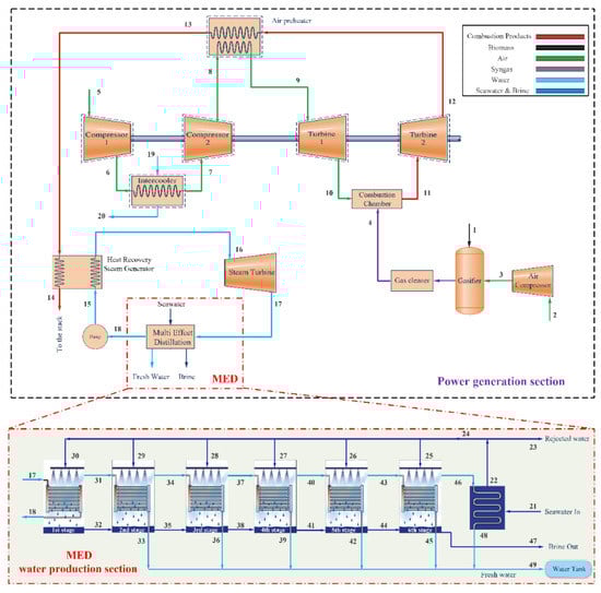
Figure 1.
Proposed integrated gasification combined cycle for electricity and water production.
The main system operation is as follows. Air is pressurized in a two-stage compressor with an intercooler between the stages. First, air enters compressor 1 at 1.013 bar and 298.15 K (the environmental condition, state 5) and is pressurized (state 6). In the compression process, the air temperature increases considerably so, to raise the net power output and potential for regeneration, the air is cooled in an intercooler (process ) which uses cooling water flow (process ) prior to entering compressor 2. The pressurized and cooled air (state 7) is compressed in the second-stage compressor to the final pressure (process ). The high-pressure air leaving compressor 2 is heated in the air preheater (regenerator) using high-temperature flue gases of the second turbine (process ). The high-pressure and high-temperature air (state 9) expands through the turbine (Turbine 1); the first-stage power generation process occurs in the gas turbine system. The hot turbine exhaust (state 10) enters the combustor.
Air is provided for the gasification process by the companion of the air compressor (AC) between states 2 and 3, and the biomass fuel enters the gasifier at state 1. After the reactions occur in the gasifier, solid wastes and other pollutants are removed in the gas cleaner unit. The produced synthesis gas (syngas) is delivered to the combustion chamber (state 4). The syngas is fired with air as the oxidant in the combustion chamber. The flue gas produced by the combustion process enters the second turbine (Turbine 2) and expands to produce electricity (process ). The outlet flue gas of the second-stage turbine at state 12 is delivered to the air preheater (regenerator), where it is cooled by transferring its energy to the air flow (process ). The exhaust gas temperature in the air preheater is still high and has a significant thermodynamic utility that can be harnessed economically. Thus, the integrated gasification unit and gas turbine cycle are combined with a steam Rankine cycle. The gas and steam power cycles are combined by an interconnecting HRSG that acts as the boiler for the Rankine power system. Finally, the flue gas is discharged to the environment at 150 °C. The corresponding diagram of the cycle is shown in Figure 2, which indicates that significant exergy destructions occur in the turbines and compressors.
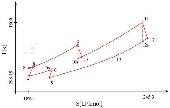
Figure 2.
T-s diagram for the integrated gasification and regenerative gas turbine cycle.
In the steam Rankine cycle, water enters the pump at state 18 as a saturated liquid and is pressurized to the boiler pressure with a slight increase in the water temperature (state 15). The compressed water enters the HRSG and, upon being heated by the combustion gases, leaves the HRSG as a superheated vapor at state 16. This superheated vapor enters the steam turbine (ST), where it expands and generates electricity (process ). During the expansion process in the steam turbine, the temperature and pressure of the steam decrease. The exhaust steam discharges to the condenser at state 17. There, steam is condensed at constant pressure by rejecting heat to a cooling media, and the saturated liquid at state 18 returns to the pump, completing the steam cycle. Among the various cooling mediums, multi-effect desalination (MED) is a good candidate for utilization instead of the condenser. Compared to widely used thermal processes such as multi-stage flash, MED desalination has advantages such as lower primary energy consumption, lower heat transfer area, lower capital cost, longer life, less corrosion, lower scaling rate, and less need for pre-filtering []. A parallel-cross heat exchanger arrangement, because it performs better in terms of energy consumption and gain output ratio (GOR) [], was used in this study. Figure 1 shows a magnified schematic of a MED unit with six effects.
The MED driving steam with a mass flow rate of at a somewhat high pressure (P17) is directed towards the first effect of the MED unit. The latent heat is used to increase the temperature of the falling seawater of the first effect to the boiling point and evaporates a section of the feedwater. The condensate returns to the pump to complete the steam Rankine cycle. The unevaporated portion of seawater is collected as brine or wastewater at the bottom of the chamber and passes to the second effect. The vapor produced in the first effect as a heat source moves to the second stage and delivers its latent heat to the falling feedwater and condenses as freshwater. As a result, part of the spray water turns to steam, and this steam passes to the next effect, and this process repeats until the last effect. For optimal use of the saline water energy, the output brine from the first effect enters the second effect to increase the feedwater temperature. The steam formed in the last effect loses its latent heat to the inlet seawater (state 21) and condenses in the condenser of the MED unit. In the condenser, the temperature of the seawater increases. Part of the seawater, with a mass flow rate of , is used as feedwater, and the remainder with a flow rate of is considered as rejected water. The motive steam that has lost its latent heat in the first effect and is converted to a saturated liquid is sent to the Rankine pump. Through this desalination process, water is purified in each effect and stored in a water tank at state 49, while the brine is collected in each state and rejected at state 47.
3. Modeling and Assumptions
3.1. Thermodynamic Assumptions
Several thermodynamic assumptions are invoked to simplify the study. These are as follows [,,]:
- The operation of each process in the cycle is considered to be at steady state.
- Changes in the potential and kinetic energy rates are ignored; thus, only physical and chemical exergies are considered.
- Pressure drops in the steam Rankine cycle are neglected, and pressure loss of the combustion chamber is taken to be 5%.
- The input air composition is 79% N2 and 21% O2.
- Also, the reference environment properties T0 and P0 are taken to be 298.15 K and 1.013 bra, respectively.
- The temperature differences for the flows in all effects of the MED are equal.
- The spray of seawater in all effects of the MED occurs in an equal flow rate.
Other primary input parameters and prerequisites for simulation of the proposed electricity and water generation plant are presented in Table 1.

Table 1.
Some input parameters and considerations for the modeling of the proposed system [,].
3.2. Thermodynamic Modeling
In this subsection, mass, energy, and exergy balances, which are applied in the assessment of the proposed cycle, are considered. Mass and energy rate balances, respectively, can be written as follows []:
Here, is the mass flow rate; denotes the specific enthalpy; and are the heat transfer rate and mechanical power.
Also, the exergy rate balance can be written as []:
The exergy of a material flow has four main parts: physical, chemical, potential, and kinetic. Variations of the velocities and heights in the elements are negligible. So, the total exergy rate for the kth stream can be expressed as []:
Note that is the physical exergy rate for all streams and can be computed by []:
Based on the materials used in the proposed cycle, the following relations can be used for the chemical exergy rate []:
where denotes the coefficient of the fuel chemical exergy [].
Detailed mass, energy, and exergy rate balance relations for each component in the system are given in Table 2.
Table 2.
Mass, energy, and exergy rate balances for components of the proposed system.
3.2.1. Gasifier
For the modeling of gasifier, the equilibrium conditions are considered for each reaction. The equilibrium condition is attained by minimization of Gibbs free energy. This method needs only as input, the elemental composition of the feedstock. Therefore, this method is mostly appropriate for biomasses, for which the chemical formula is not evident but can be obtained from ultimate analysis. Relevant reactions in the gasification process follow, where air is considered as a gasification agent [,]:
The global gasification reaction follows for the air agent []:
Here, denotes the biomass fuel; is the biomass moisture content; indicates the amount of gasification agent (in ). Atomic balances of are implemented to determine relevant factors. The final biomass analysis is as follows:
The ultimate analysis of the biomass utilized as the gasifier feedstock is used for the moisture content MC. That is,
Hence, the moisture content of the biomass is defined as:
The reaction process is considered to be at the equilibrium condition, and equilibrium constraints for Equations (10) and (11) are presented as []:
Therefore, equilibrium constants must be computed by the change in Gibbs free energy as []:
where denotes the gasification temperature. Also,
Finally, the principle of energy conservation is applied to the gasification system to obtain the air-to-fuel ratio. That is,
3.2.2. Combustion Chamber
For complete combustion, the following reaction occurs in the combustion chamber []:
Here, the coefficients to are calculated in the gasification analysis, and the coefficient denotes the oxygen mole number for combustion of the synthesis gas. For an adiabatic combustion chamber, the energy conservation equation yields:
where denotes the jth component’s molar number in the synthesis gas, air, or produced gas of the combustion chamber.
3.2.3. Heat Recovery Steam Generator (HRSG)
Figure 3 illustrates a single-pressure heat recovery steam generator and the temperature changes of hot water and hot product gas. As shown in Figure 3, the HRSG system consists of three parts: an economizer, an evaporator, and a superheater. In the economizer, the water enters at a temperature of and reaches a temperature of , which has a temperature difference with the saturation temperature as large as the approach point temperature. In the evaporator, the saturated liquid is converted to saturated vapor by receiving heat and, eventually, the saturated vapor temperature is heated to in the superheater.
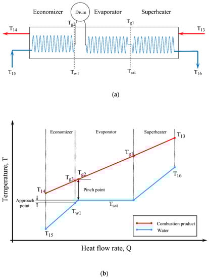
Figure 3.
(a) Schematic of a single-pressure HRSG, (b) T-Q diagram of hot water and hot product gases.
Given the above points, the following equations are used in the thermodynamic modeling of the HRSG unit []:
3.2.4. MED Desalination Unit
Figure 4 illustrates the ith effect of the MED unit.
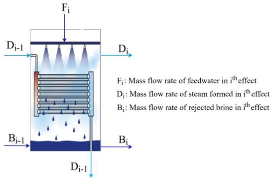
Figure 4.
th effect of MED unit.
As mentioned earlier in the assumptions, the temperature difference between the effects is constant; hence, for the th effect, the temperature difference is calculated as follows []:
Also, the temperature of brine in each stage can be defined as:
Increasing the salinity of water raises its boiling temperature; thus, the temperature of the generated vapor in each effect is lower than the boiling point of that effect. Therefore, the vapor temperature of the ith effect is given by []:
Here, denotes the boiling point elevation and the vapor temperature.
The motive flow is the steam. For the evaporators we have:
where is the rejected mass flow rate of the first effect, is the mass flow rate of steam formed in the first effect, and is the specific latent heat of evaporation.
A mass balance for salt for the first effect follows []:
Here, and denote the salinity of the supply saline water and the salinity of the rejected brine, respectively.
The conservation of mass and energy for the ith effect can be written as follows []:
The flow rate of rejected water is calculated through the following relation:
The total generated distilled water for the MED unit is:
An important parameter of the thermal desalination units is the GOR, which expresses the ratio of the generated distilled water mass to the motive steam flow rate:
3.3. Exergoeconomic Analysis
A thorough exergoeconomic evaluation is performed in Appendix A, which includes the main economic parameters for the power and water production system.
3.4. Main Performance Criteria
An evaluation metric is proposed here for the analyses of the system considered. The net output work rate is written as:
The exergy efficiency is defined as the proportion of the useful or generated exergy to the input exergy and can be expressed as:
Also, the rate of exergy loss for the proposed system is calculated as follows:
Also, the sum unit cost of product for the proposed system is expressed as:
4. Results and Discussion
Results of the modeling and analysis of the proposed electricity and freshwater production unit are presented in this section. First, a validation of mathematical models is performed. Then, the base system with basic operating parameters is defined and examined, and subsequently the impacts of various parameters on the system performance are considered and the economic results are presented.
4.1. Model Validation
A comparison is presented of results obtained here and in related works in the literature in order to validate the proposed modeling process through EES software []. Results from [,,] are utilized here to validate the gasification process. For the validation of the MED unit, the work of Hatzikioseyian et al. [] was employed. In this validation, conditions and considerations are regarded as similar to comparative references. The comparative results for the validation of the gasifier and MED units are listed in Table 3. As indicated in Table 3 for the gasification process and considering the root-mean-square deviation (RMSD) metric, the results obtained here are in very good agreement with those of experimental and also other works.
Table 3.
Model validation for gasification process and MED desalination unit.
In addition, for the validation of the MED unit, the relative error is calculated. Based on these results, it can be inferred that results for the model developed here for the MED unit agree well with results from corresponding references.
4.2. Main Operating Results
The main properties of each stream in the proposed plant for the base case are given in Table 4.
Table 4.
Values of thermodynamic and economic quantities of states for the proposed system.
The main performance criteria are presented in Table 5. For the base case, the net output power obtained is . This value is the sum of the net power outputs of the gas turbine cycle and the steam Rankine cycle. The freshwater production rate is calculated as . The exergy efficiency of the proposed plant is . The value of the sum unit cost of products (SUCP) for the plant for the base case is calculated as , while the payback period is found to be when the fuel cost is and electricity and water are sold for and , respectively. In this condition, the net present value at the end of system lifetime is calculated as $.
Table 5.
Main simulation outputs of the proposed system at base conditions.
The exergy flow rates and destruction rates of the proposed system are presented in a Sankey diagram in Figure 5. Based on Figure 5, the maximum rate of exergy destruction is attributable to the combustion chamber, mainly because of the nature of the combustion reactions and heat transfer occurring. Of the total input exergy rate of 18,237 kW, are destroyed in the combustion chamber. The second greatest exergy destruction rate () occurs in the gasifier. The value of exergy loss rates are seen in the Sankey diagram to be . Accounting for exergy destruction and loss rates, the exergy efficiency is obtained as 46.22%.
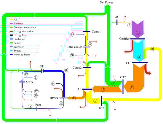
Figure 5.
Sankey diagram of the proposed system showing exergy flows and exergy destructions.
The share of each component to the total exergy destruction rate is plotted in Figure 6. The combustion chamber is responsible for of total exergy destruction rate, while the gasifier and Rankine units account for and of the total exergy destruction rate, respectively. Of the components of the Rankine subsystem, the HRSG has the largest exergy destruction rate while, in the MED subsystem, the highest exergy destruction rate is associated with the condenser.
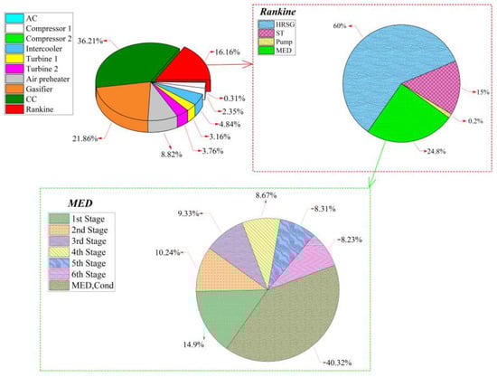
Figure 6.
Exergy destruction rate’s breakdown by components.
Table 6 presents the exergy destruction cost rate (), the investment cost rate (), the exergy destruction rate (), and the exergy efficiency (). The air preheater accounts for the highest investment cost of all system components. The Rankine cycle pump contributes the lowest portion to the system exergy destruction rate.
Table 6.
Exergy and exergoeconomic factors for the proposed system.
4.3. Parametric Analysis
The effects of varying important functional parameters on the main performance criteria for the system were examined. The range of decision variables for the parametric analysis, as well as the value of each parameter for the base case, are given in Table 7. The parametric analysis results are plotted in Figure 7, Figure 8, Figure 9, Figure 10, Figure 11, Figure 12 and Figure 13.
Table 7.
Decision variables for parametric analysis.
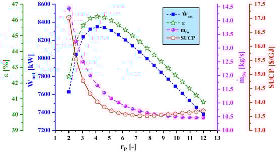
Figure 7.
Effect of compressor pressure ratio () on main performance criteria.
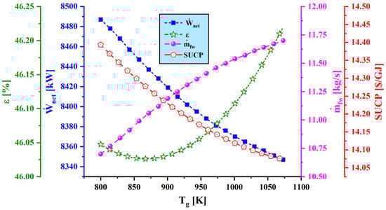
Figure 8.
Effect of gasification temperature () on main performance criteria.
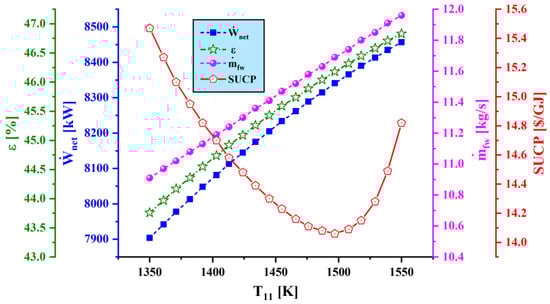
Figure 9.
Effect of varying combustion temperature () on main performance criteria.
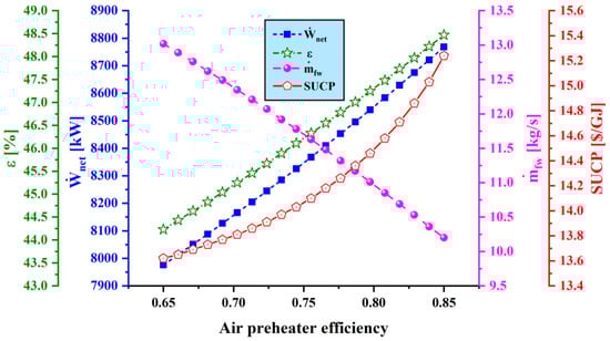
Figure 10.
Effect of air preheater effectiveness () on main performance criteria.
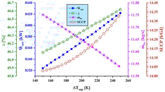
Figure 11.
Effect of superheating temperature difference () on main performance criteria.
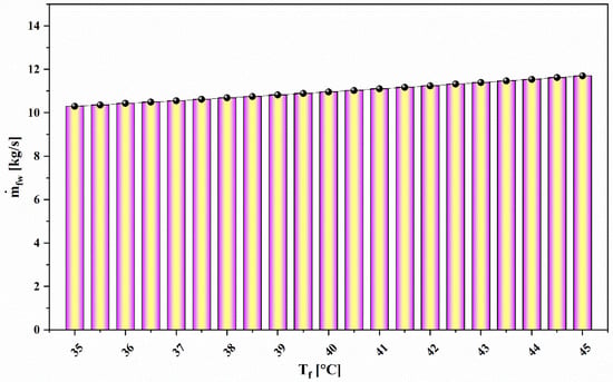
Figure 12.
Effect of feedwater temperature () on water production capacity.
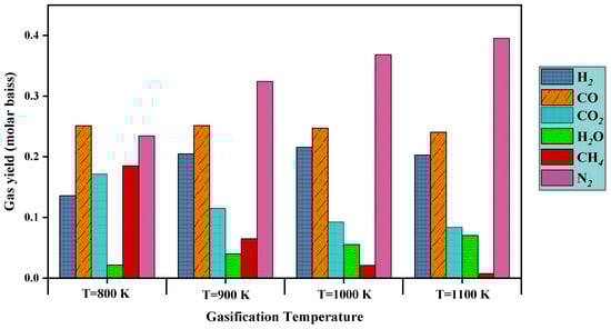
Figure 13.
Effect of gasification temperature () on gas yield.
4.3.1. Effect of Compressor Pressure Ratio on System Performance
Figure 7 shows the effect of varying compressor pressure ratio () on the main performance criteria. As the compressor pressure ratio increases, the net output power and exergy efficiency increase to a maximum value and then decrease, while the sum unit cost of product decreases to a minimum value and then increases. Also, the water production rate value drops continuously. The main reason for this trend is that, as the compressor pressure ratio increases, the exit temperature of the compressor rises. Thus, the combustion product composition varies, which leads to a higher power generation rate and consequently a higher exergy efficiency and a lower SUCP. However, increasing the compressor pressure ratio to higher values leads to a decline in the fuel mass flow rate, so the net output power and exergy efficiency decrease.
4.3.2. Effect of Gasification Temperature on System Performance
The impact of varying gasification temperature on the net output power, exergy efficiency, water production capacity, and SUCP is shown in Figure 8. Raising the gasification temperature decreases the net power output due to the decline of and formation in the output gases of the gasification process, which reduces the output power of the gas turbine. Also, an increase of gasification temperature causes more heat to be delivered to the MED system, increasing considerably the freshwater generated by the proposed system. The exergy efficiency increases as power generation decreases and freshwater generation increases. As a result, the sum unit cost of the products decreases.
4.3.3. Effect of Combustion Chamber Temperature on System Performance
Figure 9 demonstrates the trends of net output power, exergy efficiency, freshwater production rate, and SUCP as the combustion chamber temperature varies. It is seen that water generation rate and power generation increase as combustion chamber temperature rises. This trend is mainly caused by the enthalpy increase at the gas turbine inlet. Also, increasing combustion chamber temperature increases the energy delivery to the Rankine cycle and thus boosts the water production rate of the MED unit. The exergy efficiency of the overall system increases as power generation and water production capacities rise. However, the effect of the increasing of the combustion chamber temperature on the sum unit cost of the product exhibits a different trend, with SUCP decreasing to a minimum value and then increasing.
4.3.4. Effect of Air Preheater Effectiveness on System Performance
Figure 10 demonstrates the variation of net output power, exergy efficiency, freshwater production capacity, and SUCP with the air preheater efficiency. It is observed that the freshwater and power production capacity increase as air preheater efficiency rises. The reason is that, as the air preheater efficiency increases, the heat transfer rate to the air flow rises so that the inlet temperature of turbine 1 increases, which results in higher power output from turbine 1. However, as the heat transfer rate to air flow increases, the energy delivered to the Rankine cycle decreases, so the water production rate decreases. These variations in water production rate and power generation capacity lead to an increase in exergy efficiency, and ultimately, sum unit cost of the product as air preheater efficiency rises.
4.3.5. Effect of Superheating Temperature Difference on System Performance
Figure 11 shows the variation of net output power, exergy efficiency, freshwater production rate, and SUCP as superheating temperature difference () varies for the proposed system. The net power generation rate increases as the superheating temperature difference raises since the inlet temperature to the steam turbine increases, leading to a higher power production rate by the steam turbine. However, as rises, the mass flow rate of the Rankine cycle decreases slightly; hence, the motive steam flow rate decreases, yet the water production capacity decreases. Thus, exergy efficiency and SUCP increase as the output power rises and the freshwater production rate declines.
4.3.6. Effect of Feedwater Temperature () on Water Production Capacity
Figure 12 illustrates the variation of freshwater production rate with feedwater temperature () for the proposed system. The relation parallels that observed for the water production rate as feedwater temperature rises. The main reason for this increase is that, as the feedwater temperature increases, the vapor production rate in the MED effects increases considerably; hence, the water production rate increases.
4.3.7. Effect of Gasification Temperature () on Gas Yield
The effect of gasification temperature for selected biomass was studied to observe the gas yield potential at different operating temperatures. The produced components molar ratio in the temperature range to is presented in Figure 13. It is observed from the plot that hydrogen yield percentage increases with an increase in temperature up to . It is also observed from the plot that methane yield is decreased with increment of gasification temperature. Also, it is observed that produced gas compositions follow the trend as observed in the experimental investigation. Carbon dioxide and carbon monoxide molar ratio show a decreasing trend with an increase in gasification temperature.
4.4. Net Present Value and Payback Period
Figure 14 and Figure 15 illustrate the effects of electricity selling price () and fuel purchasing cost () on the NPV of the system over its lifetime. It is observed that a lower payback period and higher total NPV are attained as the electricity price increases. Figure 14 shows the variation of NPV for , , and various electricity selling prices. It can be seen that, for an electricity selling price of and lower, the total value of NPV at the end of the plant life is negative, so such a plant is not feasible from an economic viewpoint. However, for for purchasing the fuel and for selling the electricity, such a plant would be feasible from an economic perspective in most countries. For instance, for and , the total NPV value at the end of plant lifetime is . Also, based on this figure, the payback period () drops from for to for .
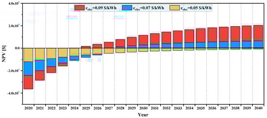
Figure 14.
Effect of electricity selling price on NPV of system over its lifetime.
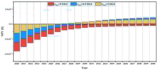
Figure 15.
Effect of fuel purchase cost on NPV of system over its lifetime.
The effect of varying fuel purchase price is shown in Figure 15, for and . It is seen that, for a fuel price higher than , the total NPV is negative at the end of the plant lifetime. So, for this plant, it takes more than years to be profitable, so it is not feasible economically. However, for a fuel cost of and lower, the plant can be profitable after some years of operation. Moreover, the payback period increases from to as the fuel cost increases from to .
5. Conclusions
A novel IGCC-based system for electricity and freshwater production was proposed and analyzed from thermodynamic and economic viewpoints. The main novelties of the devised system lie in the integration of biomass gasification with a regenerative gas turbine with intercooling and syngas combustor, and utilization of the energy discharged from the gas turbine system through an HRSG for further power generation. Another novelty of the proposed system is the combination of SRC and MED desalination units, with the latter acting as the condenser of the SRC plant. Such an arrangement results in higher thermal and exergy efficiencies than either plant would have individually.
The feasibility of the devised system was analyzed from thermodynamic and economic viewpoints. A comprehensive parametric study was carried out to evaluate the effect of some important parameters on the system’s performance. The net present value and payback period were employed to evaluate the economic feasibility of the plant. The main results and the conclusions drawn from them are as follows:
- For the base case, the system has , , and . Also, the water production rate is calculated as .
- The exergy analysis shows that, among all system components, the combustion chamber contributes the highest exergy destruction rate (), representing of the overall exergy destruction rate.
- The parametric analysis shows that increasing the gasification temperature results in lower power production.
- For a fuel cost of , a freshwater selling price of , and an electricity price of , the total NPV value at the end of plant lifetime is which means that the plant is feasible from an economic viewpoint. For these values, the payback period is . However, the payback period is sensitive to these values, increasing from to as the fuel cost increases from to .
Author Contributions
Formal analysis: F.H., A.S., S.M.S.M., B.E. and M.A.R.; Writing—original draft: A.S.; Methodology: S.M.S.M.; Writing—review & editing: M.A.R. All authors have read and agreed to the published version of the manuscript.
Funding
This research received no funding.
Conflicts of Interest
The authors declare no conflict of interest.
Nomenclature
| Symbols | |
| Area () | |
| Annual income () | |
| Approach point temperature () | |
| Annual savings () | |
| Boiling point elevation (°C) | |
| Rejected mass flow rate () | |
| Cost per unit exergy () | |
| Cost rate () | |
| Capital recovery factor | |
| Mass flow rate of steam in MED effects () | |
| Specific exergy () | |
| Exergy rate () | |
| Mass flow rate of feedwater in MED effects () | |
| Gain output ratio | |
| Gas turbine cycle | |
| Gibbs free energy ( | |
| Specific enthalpy () | |
| Heat recovery steam generator | |
| Integrated gasification combined cycle | |
| Equilibrium constant | |
| Lower heating value () | |
| Mass flow rate () | |
| Molecular weight () | |
| Multi-effect distillation | |
| Moisture content () | |
| Molar rate () | |
| Lifetime of system () | |
| Net present value () | |
| Pressure () | |
| Payback period () | |
| Pinch point temperature difference () | |
| Heat rate () | |
| Pressure ratio | |
| Universal gas constant () | |
| Specific entropy () | |
| Steam Rankine cycle | |
| Sum unit cost of product () | |
| Temperature () | |
| Total gain output ratio | |
| Heat transfer coefficient () | |
| Electricity () | |
| Waste heat recovery | |
| Salinity () | |
| Investment cost of components () | |
| Subscripts | |
| Air compressor | |
| Air preheater | |
| Approach point | |
| Combustion chamber | |
| Chemical | |
| Capital investment | |
| Condenser | |
| Control volume | |
| Destruction | |
| electricity | |
| Environmental | |
| Exergy | |
| Formation | |
| Freshwater | |
| Fuel | |
| Gas turbine | |
| Inlet | |
| Investment | |
| Isentropic | |
| component | |
| Mixer | |
| Net value | |
| Operation and maintenance | |
| Outlet | |
| Physical | |
| Product | |
| Pump | |
| Pinch point | |
| Heat transfer | |
| Regenerator | |
| Saturation | |
| Steam turbine | |
| System | |
| Thermal | |
| Total | |
| Vapor generator | |
| Work | |
| Cycle locations | |
| Dead state | |
| Greek Symbols | |
| Energy efficiency () | |
| Exergy efficiency () | |
| Maintenance factor | |
| Latent heat of vaporization () | |
Appendix A
For the system considered here, the fixed cost () comprises the system’s investment cost (). Table A1 provides the investment cost for each component of the system, where the total investment cost evaluated by the summation of investment costs of each component [] is as follows:
The investment cost of the separator and mixer in comparison to other components is negligible [].
Table A1.
Cost function equations for components of the proposed system [,].
Table A1.
Cost function equations for components of the proposed system [,].
| Component | Cost Function | Ref. Year | Cost Index |
|---|---|---|---|
| Air compressor | 1994 | 368 | |
| Compressor 1 (Com1) | 1994 | 368 | |
| Compressor 2 (Com2) | 1994 | 368 | |
| Intercooler | 2000 | 394.1 | |
| Air preheater | 1994 | 368 | |
| Gas turbine 1 (GT1) | 1994 | 368 | |
| Gas turbine 2 (GT2) | 1994 | 368 | |
| Combustion chamber | 1994 | 368 | |
| Gasifier | 1994 | 368 | |
| Steam turbine (S) | 2003 | 402 | |
| Pump | 2000 | 394.1 | |
| HRSG | 1994 | 368 | |
| MED | = 6291 [1 −], , , | 2018 | 638.1 |
| First stage | 0.16 | 2018 | 638.1 |
| Second stage | 0.16 | 2018 | 638.1 |
| Third stage | 0.16 | 2018 | 638.1 |
| Fourth stage | 0.16 | 2018 | 638.1 |
| Fifth stage | 0.16 | 2018 | 638.1 |
| Sixth stage | 0.16 | 2018 | 638.1 |
| MED condenser | = 0.04 | 2018 | 638.1 |
Note that the cost of the th element is updated for the year 2020 by employing the Chemical Engineering Plant Cost Index (CEPCI) as follows []:
The operating cost () of the plant includes the cost of operation and maintenance () and the cost of fuel (). Each of the operating cost factors is considered as follows []:
Here, is the cost of fuel and denotes the annual hours of operation for the system over its lifetime, which is considered h in this work.
Also, the cost rate balance and several auxiliary relations are used for all elements to obtain the cost rates for exergy flows. The cost rate balance for the th element of the system [] is as follows:
where
Here, is the operational and maintenance cost rate, while and denote the specific exergetic cost and cost rate, respectively. Also, is the capital recovery factor, which is defined as follows []:
Here, denotes the interest rate and the number of operational years, which is taken to be 20 years for this study.
The overall heat transfer coefficients for the heat exchangers of the proposed system are listed in Table A2.
Table A2.
Heat transfer coefficients for heat exchangers of the proposed system [].
Table A2.
Heat transfer coefficients for heat exchangers of the proposed system [].
| Component | |
|---|---|
| Intercooler | 850 |
| Air preheater | 18 |
Moreover, the cost rate balances, as well as the relevant auxiliary relations, are provided in Table A3 for each element.
Table A3.
Cost rate balances and auxiliary equations for components of the proposed system.
Table A3.
Cost rate balances and auxiliary equations for components of the proposed system.
| Component | Cost Rate Equations | Auxiliary Equations |
|---|---|---|
| Air compressor | , | |
| Compressor 1 (Com1) | , | |
| Compressor 2 (Com2) | ||
| Intercooler | ||
| Air preheater | ||
| Gas turbine 1 (GT1) | ||
| Gas turbine 2 (GT2) | ||
| Combustion chamber | - | |
| Gasifier | - | |
| Steam turbine (S) | ||
| Pump | ||
| HRSG | ||
| First stage of MED | ||
| Second stage of MED | ||
| Third stage of MED | ||
| Fourth stage of MED | ||
| Fifth stage of MED | ||
| Sixth stage of MED | ||
| MED condenser | ||
| Division point | ||
| Gathering point | + |
To evaluate the feasibility of the proposed system, two main parameters were considered: net present value (NPV) and payback period (PP) []. The parameters can be written as:
where denotes the annual net financial saving, defined as follows:
Here, denotes the total annual income.
Since the income sources of the proposed electricity and freshwater generation system are derived from selling these commodities, Table A4 provides the main cost indices and also the water and electrical power selling prices.
Table A4.
Cost indices [].
Table A4.
Cost indices [].
| Parameter | Value |
|---|---|
| Maintenance factor, | 1.06 |
| Annual number of hours, (hours) | 7000 |
| Fuel price, () | 2 |
| Plant expected life, (years) | 20 |
| Electricity price, () | 0.07 |
| freshwater price, () | 1.8 |
| CEPCI for 2020 | 668 |
| Interest rate, () | 15 |
References
- Liu, B.; Rajagopal, D. Life-cycle energy and climate benefits of energy recovery from wastes and biomass residues in the United States. Nat. Energy 2019, 4, 700–708. [Google Scholar] [CrossRef]
- Tonini, D.; Hamelin, L.; Alvarado-Morales, M.; Astrup, T.F. GHG emission factors for bioelectricity, biomethane, and bioethanol quantified for 24 biomass substrates with consequential life-cycle assessment. Bioresour. Technol. 2016, 208, 123–133. [Google Scholar] [CrossRef]
- Yao, Z.; You, S.; Ge, T.; Wang, C.-H. Biomass gasification for syngas and biochar co-production: Energy application and economic evaluation. Appl. Energy 2018, 209, 43–55. [Google Scholar] [CrossRef]
- Gambarotta, A.; Morini, M.; Zubani, A. A non-stoichiometric equilibrium model for the simulation of the biomass gasification process. Appl. Energy 2018, 227, 119–127. [Google Scholar] [CrossRef]
- Weil, K.S. Coal gasification and IGCC technology: A brief primer. Proc. Inst. Civ. Eng. Energy 2010, 163, 7–16. [Google Scholar] [CrossRef]
- Parraga, J.; Khalilpour, K.R.; Vassallo, A. Polygeneration with biomass-integrated gasification combined cycle process: Review and prospective. Renew. Sustain. Energy Rev. 2018, 92, 219–234. [Google Scholar] [CrossRef]
- Sahraei, M.H.; McCalden, D.; Hughes, R.W.; Ricardez-Sandoval, L. A survey on current advanced IGCC power plant technologies, sensors and control systems. Fuel 2014, 137, 245–259. [Google Scholar] [CrossRef]
- Soltani, S.; Mahmoudi, S.M.S.; Yari, M.; Rosen, M. Thermodynamic analyses of an externally fired gas turbine combined cycle integrated with a biomass gasification plant. Energy Convers. Manag. 2013, 70, 107–115. [Google Scholar] [CrossRef]
- Gholamian, E.; Mahmoudi, S.M.S.; Zare, V. Proposal, exergy analysis and optimization of a new biomass-based cogeneration system. Appl. Therm. Eng. 2016, 93, 223–235. [Google Scholar] [CrossRef]
- Ahmadi, P.; Rosen, M.A.; Dincer, I. Multi-objective exergy-based optimization of a polygeneration energy system using an evolutionary algorithm. Energy 2012, 46, 21–31. [Google Scholar] [CrossRef]
- Köse, Ö.; Koç, Y.; Yağlı, H. Performance improvement of the bottoming steam Rankine cycle (SRC) and organic Rankine cycle (ORC) systems for a triple combined system using gas turbine (GT) as topping cycle. Energy Convers. Manag. 2020, 211, 112745. [Google Scholar]
- Wang, J.; Dai, Y.; Gao, L. Exergy analyses and parametric optimizations for different cogeneration power plants in cement industry. Appl. Energy 2009, 86, 941–948. [Google Scholar] [CrossRef]
- Singh, O.K.; Kaushik, S.C. Reducing CO2 emission and improving exergy based performance of natural gas fired combined cycle power plants by coupling Kalina cycle. Energy 2013, 55, 1002–1013. [Google Scholar] [CrossRef]
- Cao, L.; Wang, J.; Dai, Y. Thermodynamic analysis of a biomass-fired Kalina cycle with regenerative heater. Energy 2014, 77, 760–770. [Google Scholar] [CrossRef]
- Qi, C.-H.; Feng, H.-J.; Lv, Q.-C.; Xing, Y.-L.; Li, N. Performance study of a pilot-scale low-temperature multi-effect desalination plant. Appl. Energy 2014, 135, 415–422. [Google Scholar] [CrossRef]
- Ghaffour, N.; Bundschuh, J.; Mahmoudi, H.; Goosen, M.F. Renewable energy-driven desalination technologies: A comprehensive review on challenges and potential applications of integrated systems. Desalination 2015, 356, 94–114. [Google Scholar] [CrossRef]
- Al-Karaghouli, A.; Kazmerski, L.L. Energy consumption and water production cost of conventional and renewable-energy-powered desalination processes. Renew. Sustain. Energy Rev. 2013, 24, 343–356. [Google Scholar] [CrossRef]
- Al-Mutaz, I.; Wazeer, I. Comparative performance evaluation of conventional multi-effect evaporation desalination processes. Appl. Therm. Eng. 2014, 73, 1194–1203. [Google Scholar] [CrossRef]
- Saldivia, D.; Rosales, C.; Barraza, R.; Cornejo, L. Computational analysis for a multi-effect distillation (MED) plant driven by solar energy in Chile. Renew. Energy 2019, 132, 206–220. [Google Scholar] [CrossRef]
- Razmi, A.R.; Soltani, M.; Tayefeh, M.; Torabi, M.; Dusseault, M. Thermodynamic analysis of compressed air energy storage (CAES) hybridized with a multi-effect desalination (MED) system. Energy Convers. Manag. 2019, 199, 112047. [Google Scholar] [CrossRef]
- Baccioli, A.; Antonelli, M.; Desideri, U.; Grossi, A. Thermodynamic and economic analysis of the integration of Organic Rankine Cycle and Multi-Effect Distillation in waste-heat recovery applications. Energy 2018, 161, 456–469. [Google Scholar] [CrossRef]
- Mokhtari, H.; Sepahvand, M.; Fasihfar, A. Thermoeconomic and exergy analysis in using hybrid systems (GT+ MED+ RO) for desalination of brackish water in Persian Gulf. Desalination 2016, 399, 1–15. [Google Scholar] [CrossRef]
- Dastgerdi, H.R.; Whittaker, P.; Chua, H.T. New MED based desalination process for low grade waste heat. Desalination 2016, 395, 57–71. [Google Scholar] [CrossRef]
- Wang, Y.; Lior, N. Performance analysis of combined humidified gas turbine power generation and multi-effect thermal vapor compression desalination systems—Part 1: The desalination unit and its combination with a steam-injected gas turbine power system. Desalination 2006, 196, 84–104. [Google Scholar] [CrossRef]
- Al-Sahali, M.; Ettouney, H. Developments in thermal desalination processes: Design, energy, and costing aspects. Desalination 2007, 214, 227–240. [Google Scholar] [CrossRef]
- Rostamzadeh, H.; GhiasiRad, H.; Amidpour, M.; Amidpour, Y. Performance enhancement of a conventional multi-effect desalination (MED) system by heat pump cycles. Desalination 2020, 477, 114261. [Google Scholar] [CrossRef]
- Tsatsaronis, B.A.G.; Moran, M.J. Thermal Design and Optimization; John Wiley & Sons: New York, NY, USA, 1995. [Google Scholar]
- Sayyaadi, H.; Saffari, A. Thermoeconomic optimization of multi effect distillation desalination systems. Appl. Energy 2010, 87, 1122–1133. [Google Scholar] [CrossRef]
- Ahmadi, S.; Ghaebi, H.; Shokri, A. A comprehensive thermodynamic analysis of a novel CHP system based on SOFC and APC cycles. Energy 2019, 186, 115899. [Google Scholar] [CrossRef]
- Singh, O.K. Performance enhancement of combined cycle power plant using inlet air cooling by exhaust heat operated ammonia-water absorption refrigeration system. Appl. Energy 2016, 180, 867–879. [Google Scholar] [CrossRef]
- Behzadi, A.; Houshfar, E.; Gholamian, E.; Ashjaee, M.; Habibollahzade, A. Multi-criteria optimization and comparative performance analysis of a power plant fed by municipal solid waste using a gasifier or digester. Energy Convers. Manag. 2018, 171, 863–878. [Google Scholar] [CrossRef]
- Mehrabadi, Z.K.; Boyaghchi, F.A. Thermodynamic, economic and environmental impact studies on various distillation units integrated with gasification-based multi-generation system: Comparative study and optimization. J. Clean. Prod. 2019, 241, 118333. [Google Scholar] [CrossRef]
- Boyaghchi, F.A.; Chavoshi, M.; Sabeti, V. Multi-generation system incorporated with PEM electrolyzer and dual ORC based on biomass gasification waste heat recovery: Exergetic, economic and environmental impact optimizations. Energy 2018, 145, 38–51. [Google Scholar] [CrossRef]
- Moran, M.J.; Shapiro, H.N.; Boettner, D.D.; Bailey, M.B. Fundamentals of Engineering Thermodynamics; John Wiley & Sons: New York, NY, USA, 2010. [Google Scholar]
- Aklilu, B.; Gilani, S. Mathematical modeling and simulation of a cogeneration plant. Appl. Therm. Eng. 2010, 30, 2545–2554. [Google Scholar] [CrossRef]
- Herold, K.; Radermacher, R.; Klein, S. Engineering Equation Solver; F-Chart Software: Madison, WI, USA, 2002. [Google Scholar]
- Zainal, Z.; Ali, R.; Lean, C.; Seetharamu, K. Prediction of performance of a downdraft gasifier using equilibrium modeling for different biomass materials. Energy Convers. Manag. 2001, 42, 1499–1515. [Google Scholar] [CrossRef]
- Alauddin, Z.A. Performance and Characteristics of a Biomass Gasifier System. Ph.D. Thesis, University of Wales, Cardiff, UK, 1996. [Google Scholar]
- Vidali, H.A.R.; Kousi, P. Modelling and Thermodynamic Analysis of a Multi Effect Distillation (MED) Plant for Seawater Desalination; National Technical University of Athens (NTUA): Athens, Greece, 2003. [Google Scholar]
- CEPCI. The Chemical Engineering Plant Cost Index n.d. 2020. Available online: https://www.chemengonline.com (accessed on 27 September 2020).
- Moghimi, M.; Emadi, M.; Ahmadi, P.; Moghadasi, H. 4E analysis and multi-objective optimization of a CCHP cycle based on gas turbine and ejector refrigeration. Appl. Therm. Eng. 2018, 141, 516–530. [Google Scholar] [CrossRef]
© 2020 by the authors. Licensee MDPI, Basel, Switzerland. This article is an open access article distributed under the terms and conditions of the Creative Commons Attribution (CC BY) license (http://creativecommons.org/licenses/by/4.0/).